Case Study on Housing Demand Post-Katrina môn Kinh tế vi mô | Trường Đại học Kinh Tế Quốc Dân

CASE 1
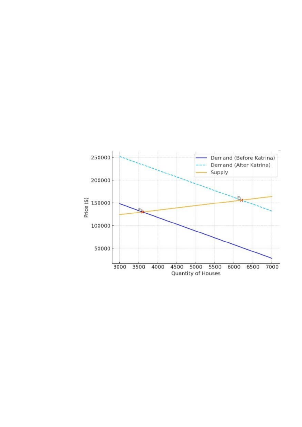
1. The arrival of approximately 250,000 displaced residents from New Orleans in the
aftermath of Hurricane Katrina caused a significant increase in the demand for
housing in Baton Rouge. (The increase in the city’s population shifted the demand curve to the right)
Demand for housing: The influx of people seeking immediate housing shifted the
demand curve to the right. This shift created a situation of a shortage at the original
average price of $130,000. The number of homes available dropped from 3,600 before
the storm to only 500 a week after, further exacerbating the shortage => supply curve (S) was relatively inelastic Price and Quantity of Housing:
-Price Increase: The average price of a single-family home rose from the initial
$130,000 to $156,000 six months later.
-Quantity: The quantity of housing likely increased modestly, due to the limited and
relatively fixed supply (S) of existing homes available for sale.
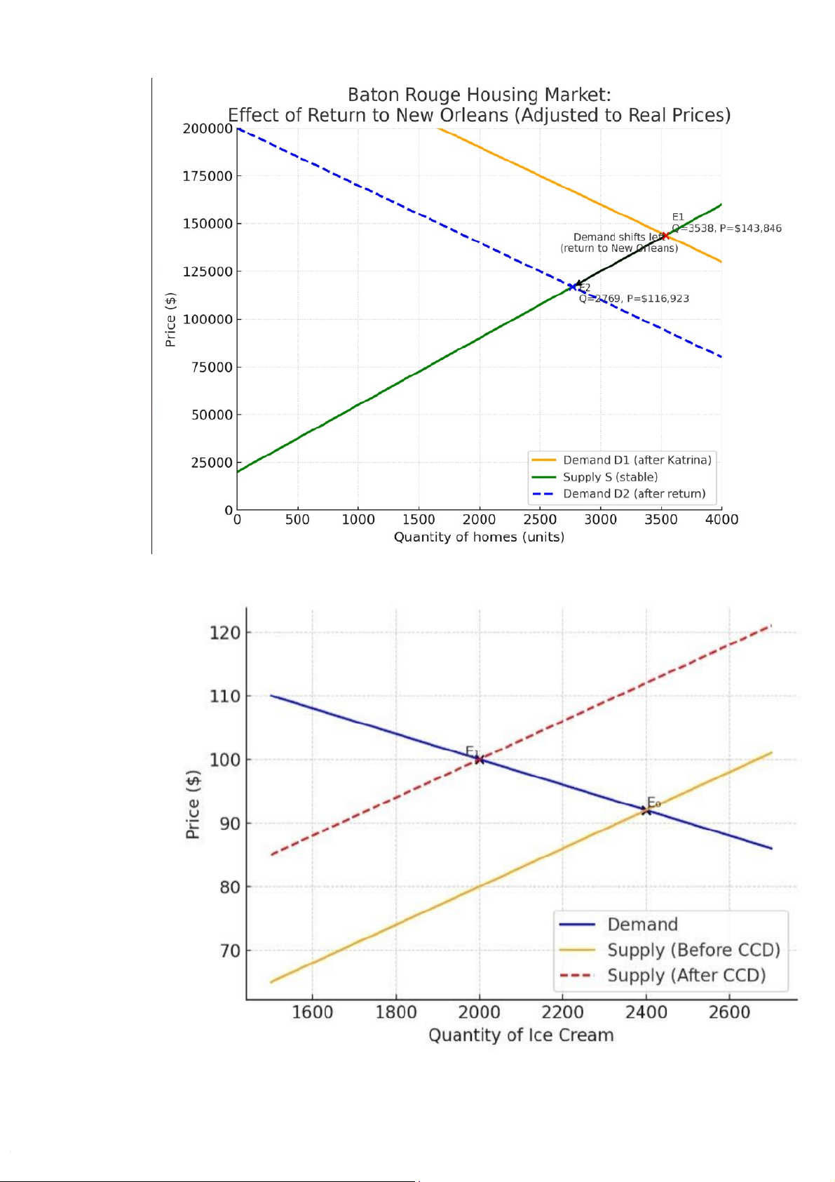
2. Five years after Hurricane Katrina, half of the people who had relocated to Baton
Rouge moved back to New Orleans. This caused the demand for housing in Baton
Rouge to decrease. As shown in the graph, the demand curve shifted leftward from D1
to D2, leading to a lower equilibrium price (P₂) and quantity (Q₂). CASE 2
After the CCD, the cost of production increased, causing the supply curve to shift
leftward. As a result, the new equilibrium shows a higher price and a lower quantity of ice cream in the market. CASE 3: a. Qold = 1, Qnew = 3. =3−1 1=2 %ΔQ 1= 2 = 200%. +) Pold = $10, Pnew = $5. %ΔP =5−10 10 =−510 = −0.5 = −50%. Elasticity= | 2
−0,5 |= 4 >1 = > Elastics .
b. Impact of promotional vouchers on monthly expenditure Before the promotion:
Expenditure1= P1× Q1= 10 × 1 = $10 After the promotion:
Expenditure2= P2× Q2= 5 × 3 = $15 
Monthly expenditure increased from $10 to $15 (+50%), it means Binh family eats
out more frequently, total spending rises.
Since |E| = 4 (> 1), demand is elastic.
->When price decreases, total expenditure increases.
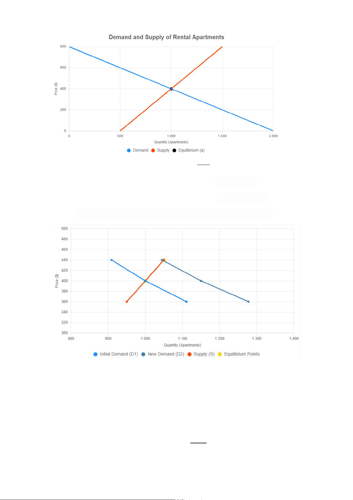
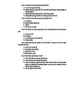
-> The result is consistent with the elasticity value. CASE 4: a. P = 800 - 0.4Qd P = 0.8Qs - 400
b. Percentage change in equilibrium price = 15% 1+0.5 = 10%
Percentage change in equilibrium quantity = 0.5 × 10% = 5%
Equilibrium price and quantity: P = $400 + ( $400 × 10%) = $440 Q = 1000 + (1000 × 5%) = 1050
c. A 15% increase in demand means at the initial price of $400, quantity demanded
rises from 1,000 to 1,000 × 1.15 = 1150 apartments.
The increase in demand by 15% will raise the equilibrium price of apartments by 10%, from $400 to $440. CASE 5:
Percentage change in equilibrium price = 24% 0.7+2.3 = 8%
Equilibrium price = $100 + ($100 × 8%) = $108
=> The import restrictions decrease the supply of steel by 24%, increasing the
equilibrium price from $100 to $108 per unit