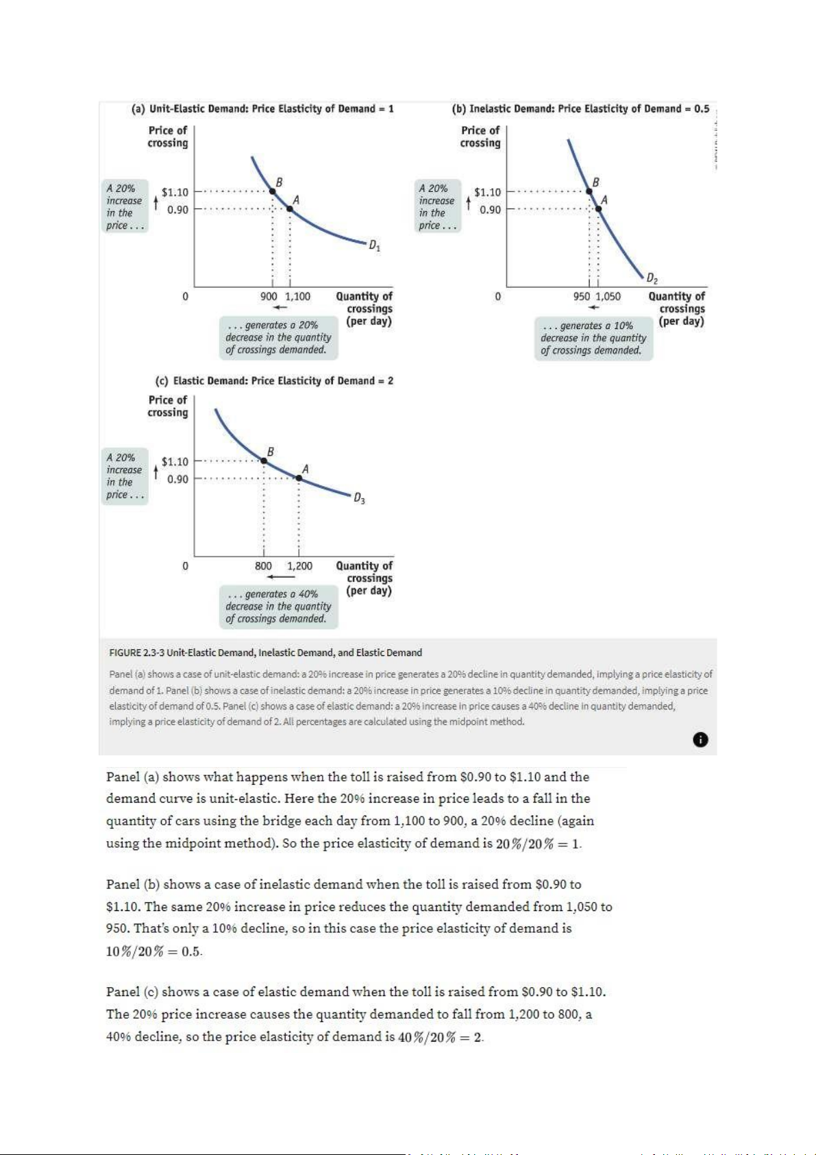
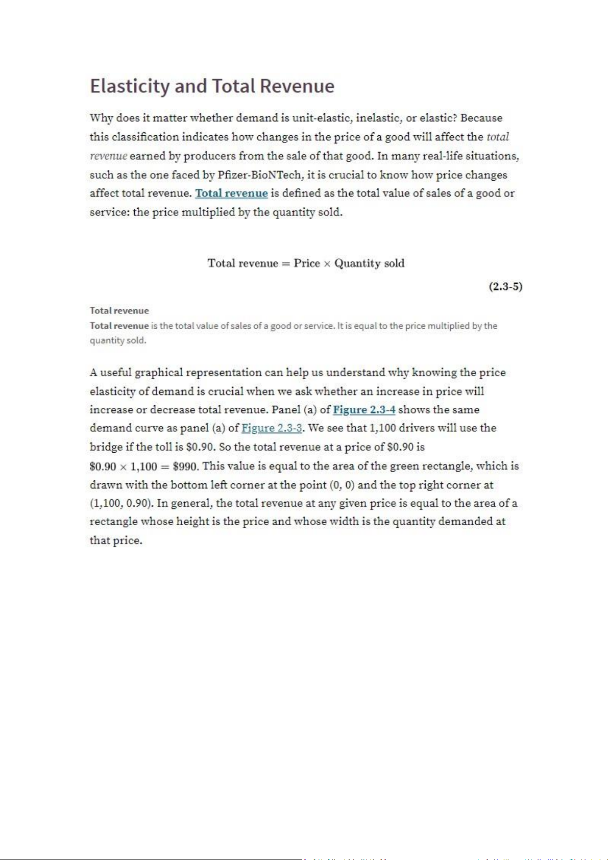
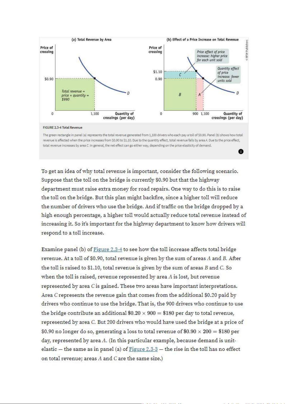
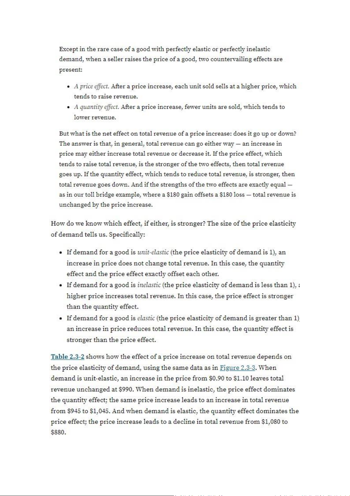
Chapter 2 OCT 5 - Practice- Trường Đại học Ngoại ngữ- Đại học Quốc gia Hà Nội

Chapter 2 OCT 5 - Practice do Trường Đại học Ngoại ngữ- Đại học Quốc gia Hà Nội tổng hợp và biên soạn.Tài liệu giúp bạn tham khảo, ôn tập, củng cố kiến thức và đạt kết quả cao trong kỳ thi sắp tới. Mời bạn đọc đón xem!

Thông tin:
22 trang 2 tuần trước

Bình luận

Vui lòng đăng nhập hoặc đăng ký để gửi bình luận.

Chapter 2 OCT 5 - Practice- Trường Đại học Ngoại ngữ- Đại học Quốc gia Hà Nội

Chapter 2 OCT 5 - Practice do Trường Đại học Ngoại ngữ- Đại học Quốc gia Hà Nội tổng hợp và biên soạn.Tài liệu giúp bạn tham khảo, ôn tập, củng cố kiến thức và đạt kết quả cao trong kỳ thi sắp tới. Mời bạn đọc đón xem!

lOMoARcPSD| 47882337
How Consumers Respond to Price Changes
The shape of the demand curve indicates how a price change aects the quanty of a good or
service that consumers demand. Consumer responsiveness to price changes is so important that it
has its own measure: the price elascity of demand. We will calculate the price elascity of demand
and see why this elascity maers to all sorts of pricing decisions. The price elascity of demand is
only one of a family of related concepts that we will nd useful as we study consumers’ and
producers’ responses to changes, including the income elascity of demand, the price elascity of
supply, and the cross-price elascity of demand.
We begin with the substuon and income eects, which give the demand curve its shape.
The Substuon Eect
When the price of a good increases, an individual will normally buy less of that good and more of
other goods. And when the price of a good decreases, an individual will normally buy more of that
good and less of other goods. This explains why the individual demand curve, which relates an
individual’s consumpon of a good to the price of that good, normally obeys the law of demand and
slopes downward.
Another way to think about why demand curves slope downward is to focus on opportunity costs.
For simplicity, let’s suppose there are only two goods between which to choose: Good 1 and Good 2.
When the price of Good 1 decreases, an individual doesn’t have to give up as many units of Good 2
in order to buy one more unit of Good 1. That makes it aracve to buy more of Good 1, whose
price has gone down. Conversely, when the price of Good 1 increases, one must give up more units
of Good 2 to buy one more unit of Good 1, so consuming Good 1 becomes less aracve and the
consumer buys fewer.
The change in the quanty demanded as the good that has become relavely cheaper is substuted
for the good that has become relavely more expensive is known as the substuon eect. When a
good absorbs only a small share of the typical consumers income, as with pillowcases and kites, the
substuon eect is essenally the sole explanaon of why the market demand curve slopes
downward. However, there are some goods, like food and housing, that account for a substanal
share of many consumers’ incomes. In such cases, another eect, called the income eect, also
comes into play.
substuon eect
The substuon eect of a change in the price of a good is the change in the quanty of that good
demanded as the consumer substutes the good that has become relavely cheaper for the good
that has become relavely more expensive.
The Income Eect
lOMoARcPSD| 47882337
Consider the case of a family that spends half of its income on rental housing. Now suppose that the
price of housing increases everywhere. This change will have a substuon eect on the family’s
demand: other things equal, the family will have an incenve to consume less housing — say, by
moving to a smaller apartment — and more of other goods. But, in a real sense, the family will also
be made poorer by that higher housing price — its income will buy less housing than before. When
income is adjusted to reect its true purchasing power, it is called real income, in contrast to money
income or nominal income, which has not been adjusted.
This reducon in a consumer’s real income will have an addional eect, beyond the substuon
eect, on the amount of housing and other goods the family chooses to buy. The income eect of a
change in the price of a good is the change in the quanty of that good demanded that results from
a change in the overall purchasing power of the consumers income when the price of the good
changes.
income eect
The income eect of a change in the price of a good is the change in the quanty of that good
demanded that results from a change in the consumers purchasing power when the price of the
good changes
AP® ECON TIP
When two terms are similar, you can more easily disnguish them by looking at the denions next
to each other: The substuon eect comes from a change in the price of one good relave to the
price of another good. The income eect of a price change comes from a change in the purchasing
power of income. An income eect can also result from a change in the actual income received.
For the majority of goods, the income eect of a price change is not important and has no signicant
eect on individual consumpon. Thus, most market demand curves slope downward solely because
of the substuon eect — end of story. When it does maer, the income eect usually reinforces
the substuon eect. That is, when the price rises on a good that absorbs a substanal share of
income, consumers of that good feel poorer because their purchasing power falls. And for all normal
goods — goods for which demand decreases when income falls — this reducon in real income leads
to a reducon in the quanty demanded and reinforces the substuon eect.
Module 2.1 introduced both normal goods and inferior goods — those goods, such as canned meat
and ramen noodles, for which demand increases when income falls. In the case of an inferior good,
the income and substuon eects work in opposite direcons. For example, suppose the price of
canned meat increases. The resulng substuon eect is a decrease in the quanty of canned meat
demanded, because for both normal and inferior goods, the substuon eect of a price increase is
a decrease in the quanty demanded of the good whose price has risen. But the income eect of a
price increase for canned meat is an increase in the quanty demanded. This makes sense because
the price increase lowers the real income of the consumer, and as real income decreases, the
demand for an inferior good increases.
lOMoARcPSD| 47882337
Could the total eect of a price increase — the combinaon of the income eect and the substuon
eect — ever be an increase in the quanty demanded? In other words, might we see an increase in
the price of ramen noodles lead to an increase in the quanty of ramen noodles demanded? It is
conceivable. If a good were so inferior that the income eect exceeded the substuon eect, an
increase in the price of that good would lead to an increase in the quanty of that good that is
demanded. There is controversy over whether such goods, known as “Gien goods,” exist at all. If
they do, they are very rare. You can generally assume that the income eect for an inferior good is
smaller than the substuon eect, and so a price increase will lead to a decrease in the quanty
demanded. Next, we will discuss elascity as a measure of the responsiveness of the quanty
demanded to price changes.
Dening and Measuring Elascity
If the price of a good or service increases, we know from the law of demand that the quanty
demanded will decrease. But by how much will the quanty demanded decrease if the price goes
up? A rm considering a price change would certainly want to know! Economists use the price
elascity of demand to measure the responsiveness of the quanty demanded to changes in the
price. Elascity can also be used to measure the responsiveness of any other variable to changes in a
related variable. We will start by looking at the price elascity of demand and then consider three
other types of elascies in the next two Modules.
Consider a pharmaceucal company that would like to know whether it could raise its revenue by
raising the price of its drugs. To know this, the company would have to know whether the price
increase would decrease the quanty demanded by a lot or a lile. That is, it would have to know
the price elascity of demand for its products.
Calculang the Price Elascity of Demand
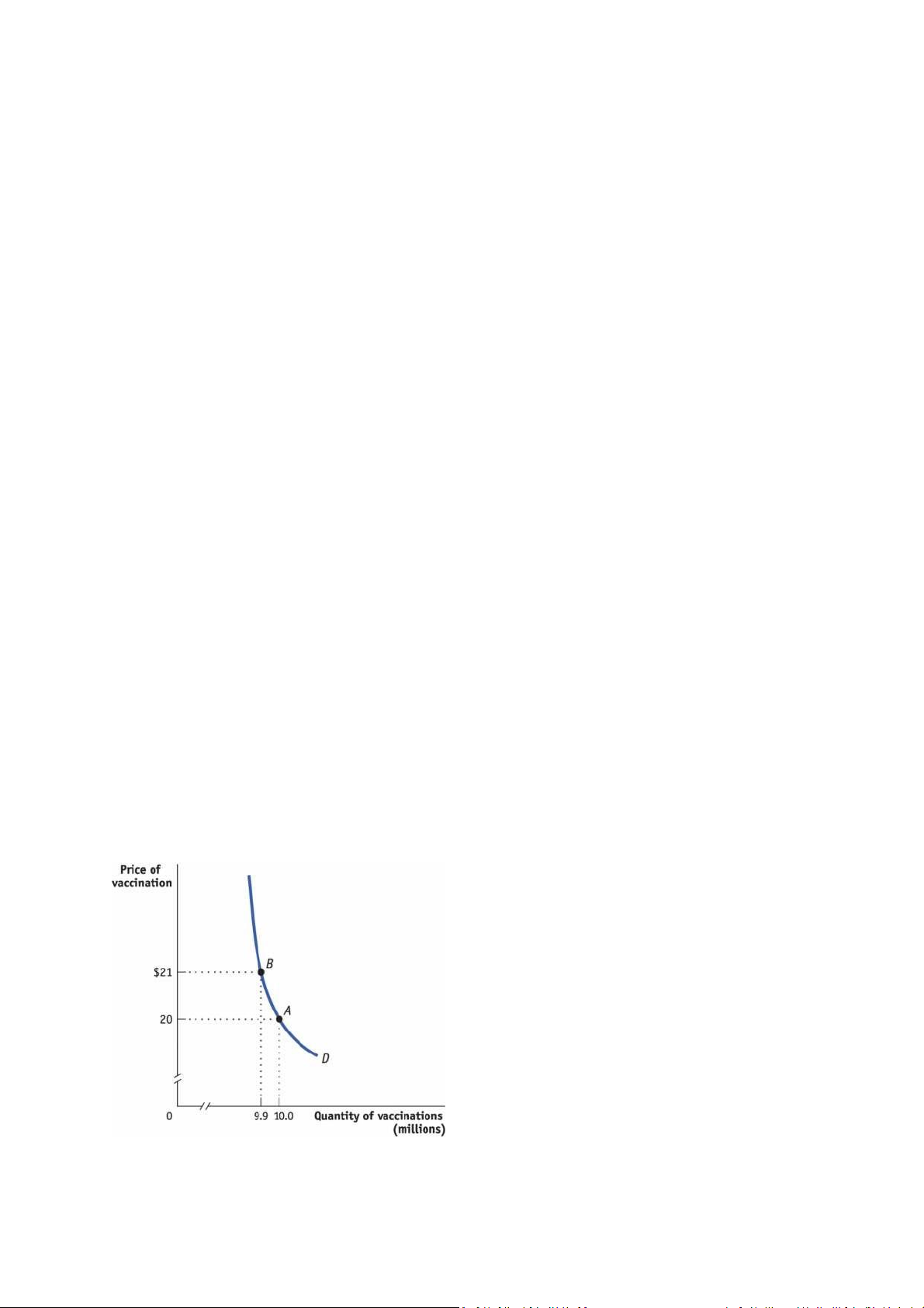
Figure 2.3-1 shows a hypothecal demand curve for a potenally life-saving medical product
purchased by millions of Americans each year, u vaccinaons. At a price of $20 per vaccinaon,
consumers would demand 10 million vaccinaons per year (point A); at a price of $21, the quanty
demanded would fall to 9.9 million vaccinaons per year (point B).
Figure 2.3-1, then, tells us the change in the quanty demanded for a parcular change in the price.
But how can we turn this informaon into a measure of price responsiveness? The answer is to
lOMoARcPSD| 47882337
calculate the price elascity of demand. The price elascity of demand compares the percentage
change in quanty demanded to the percentage change in price as we move along the demand
curve. As we’ll see later, economists use percentage changes to get a measure that doesn’t depend
on the units involved (say, a child-sized dose versus an adult-sized dose of vaccine). But before we
get to that, lets look at how elascity is calculated.
price elascity of demand
The price elascity of demand is the rao of the percentage change in the quanty demanded to the
percentage change in the price as we move along the demand curve (dropping the minus sign).
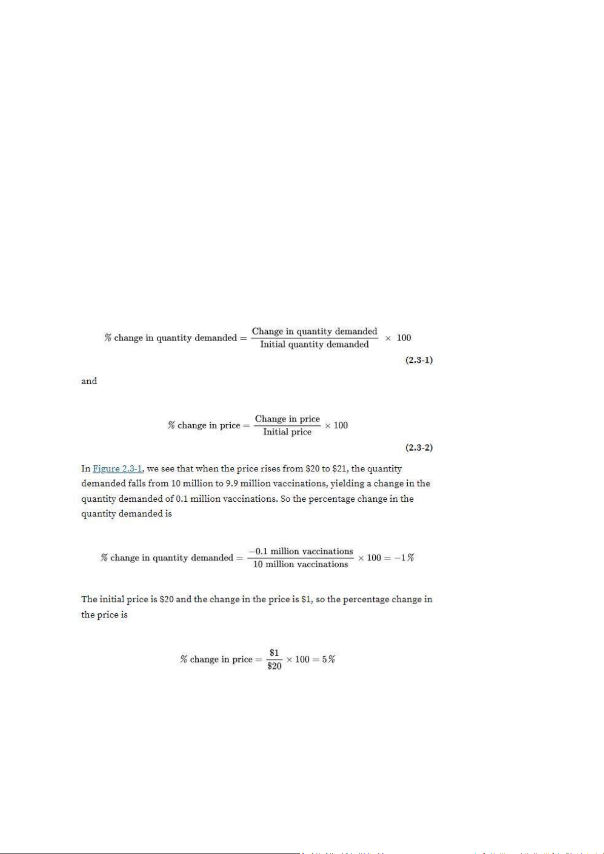
To calculate the price elascity of demand, we rst calculate the percentage change in the quanty
demanded and the corresponding percentage change in the price as we move along the demand
curve. The easiest way to do this, which we will describe as the simple method to disnguish it from
the midpoint method to be discussed a bit later, is as follows:
lOMoARcPSD| 47882337
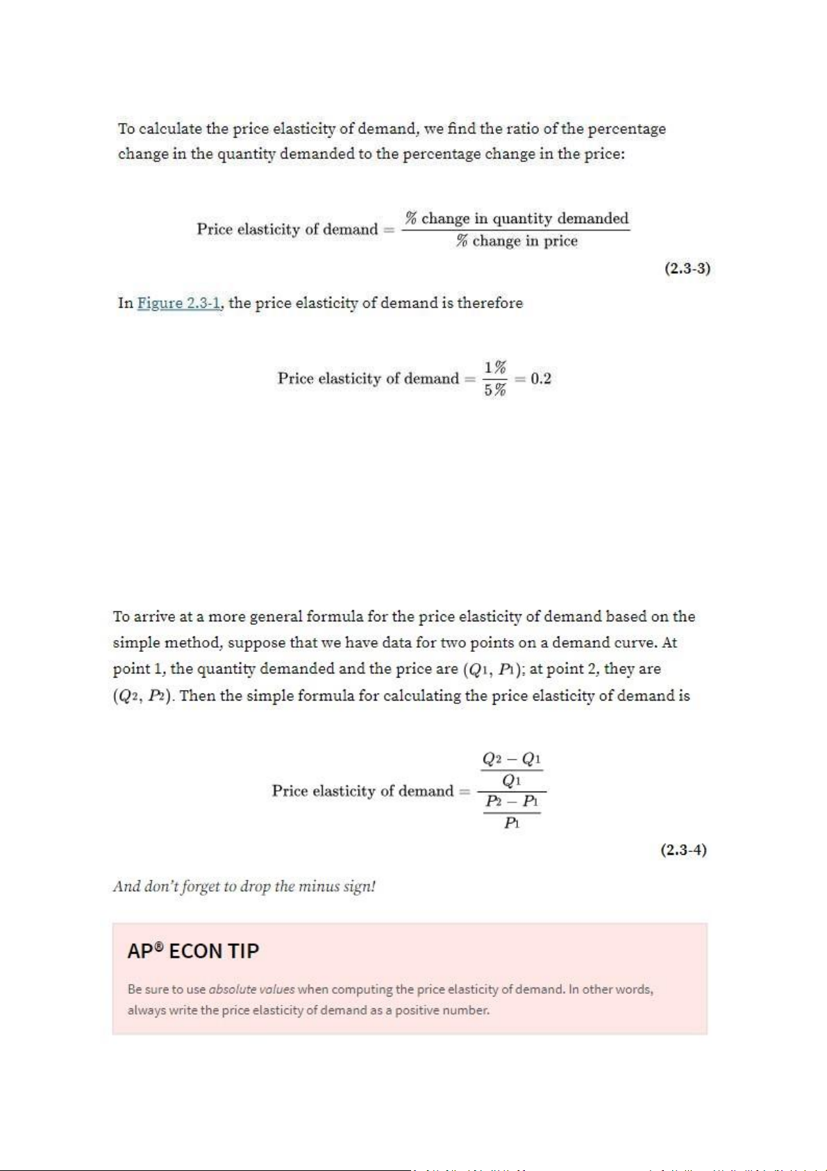
Noce that we have dropped the minus sign that had been on the percentage change in quanty.
The law of demand tells us that a posive percentage change in the price (a rise in the price) leads to
a negave percentage change in the quanty demanded, and a negave percentage change in the
price (a fall in the price) leads to a posive percentage change in the quanty demanded. This makes
the price elascity of demand a negave number. However, when economists talk about the price
elascity of demand, they usually drop the minus sign for convenience and report the absolute value
of the price elascity of demand. In this case, for example, economists would usually say “the price
elascity of demand is 0.2,” a kind of shorthand for minus 0.2. We follow that convenon here.
lOMoARcPSD| 47882337
The larger the price elascity of demand, the more responsive the quanty demanded is to the price.
When the price elascity of demand is large — when consumers change their quanty demanded by
a large percentage compared with the percentage change in the price — economists say that
demand is highly elasc.
As we’ll see shortly, a price elascity of 0.2 indicates a small response of the quanty demanded to
the price. That is, the quanty demanded will fall by a relavely small amount when the price rises.
This is what economists call inelasc demand. Later in this Module, we’ll see why inelasc demand is
exactly what a pharmaceucal company needs to succeed with a strategy to increase revenue by
raising the price of its u vaccines.
An Alternave Way to Calculate Elascies: The Midpoint Method
At this point we need to discuss a technical issue that arises when you calculate percentage changes
in variables and how economists deal with it. In our previous example, we found an elascity of
demand for vaccinaons of 0.200 when considering a movement from point A to point B. However,
when going from point B to point A, the same elascity formula would indicate an elascity of 0.212
(for useful pracce, try this calculaon). This is a nuisance: we’d like to have an elascity measure
that doesn’t depend on the direcon of change. A good way to avoid compung dierent elascies
for rising and falling prices is to use the midpoint method (somemes called the arc method).
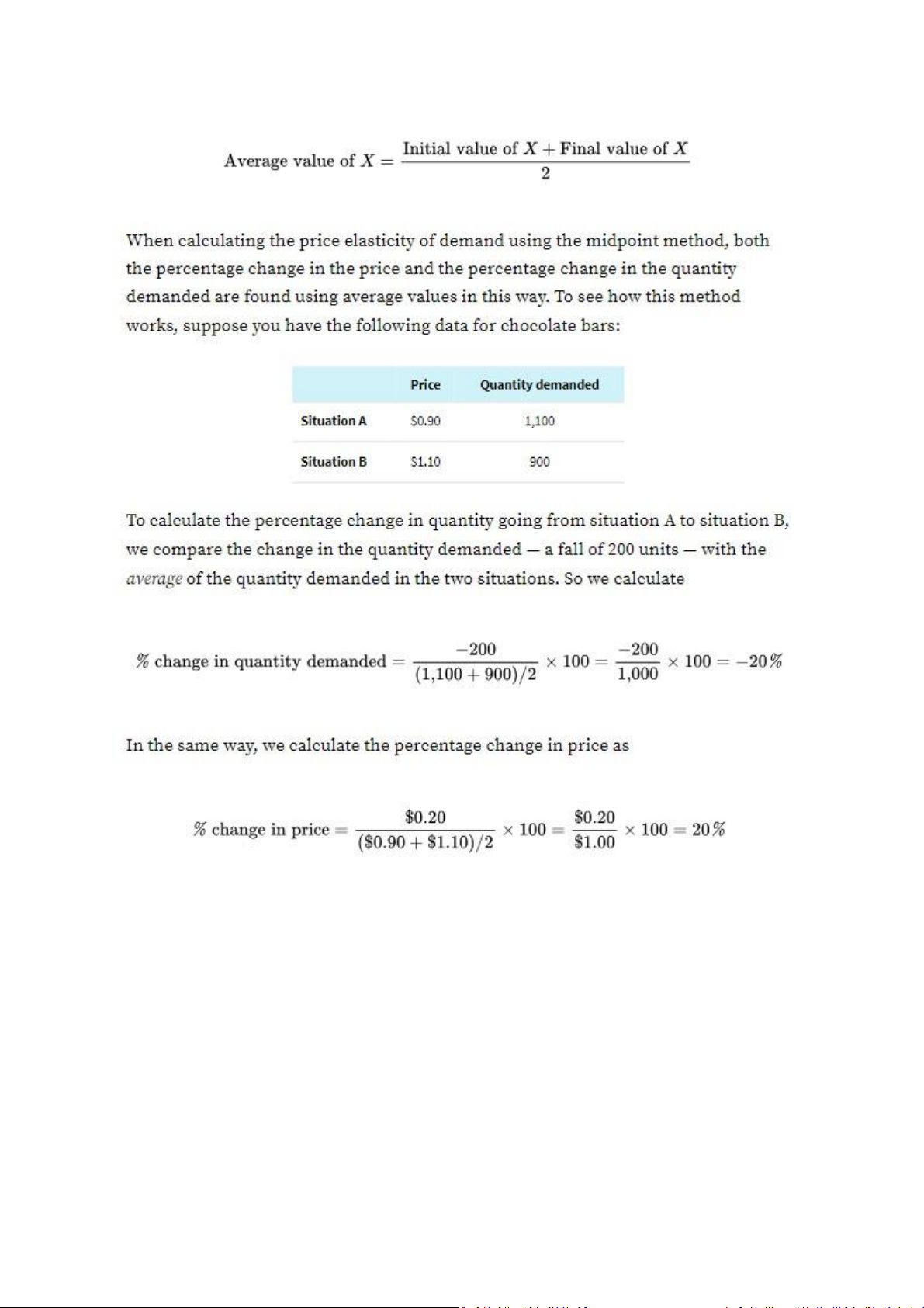
Using the midpoint method, we calculate the percentage change by dividing the change in a variable
by the average, or midpoint, of the inial and nal values of that variable. So the average value of a
variable, X, is dened as
lOMoARcPSD| 47882337
Elascity Esmates
In 1970, economists Hendrik S. Houthakker and Lester D. Taylor published a comprehensive study
that esmated the price elascies of demand for a wide variety of goods. Some of their results are
summarized in Table 2.3-1. These esmates show a wide range of price elascies. There are some
goods, such as eggs, for which demand hardly responds at all to changes in the price; there are other
goods, most notably foreign travel, for which the quanty demanded is very sensive to the price.
lOMoARcPSD| 47882337
What the Price Elascity of Demand Tells Us
Well into the coronavirus pandemic, Pzer-BioNTech raised the price of its COVID-19 vaccine by
about 25% in some countries because the price elascity of demand was low. But what does that
mean? How low does a price elascity have to be for it to be classied as low? How high does it have
to be for it to be considered high? And what determines whether the price elascity of demand is
high or low? To answer these quesons, we need to look more deeply at the price elascity of
demand.
How Elasc Is Elasc?
As a rst step toward classifying price elascies of demand, lets look at two extreme cases. First,
consider the demand for a good when people pay no aenon to its price. Suppose, for example,
lOMoARcPSD| 47882337
that consumers would buy 1 million heart bypass surgeries per year regardless of the price. If that
were true, the demand curve for these surgeries would look like the curve shown in panel (a) of
Figure 2.3-2: it would be a vercal line at 1 million heart bypass surgeries. Since the percentage
change in the quanty demanded is zero for any change in the price, the price elascity of demand
in this case is zero. The case of a zero price elascity of demand is known as perfectly inelasc
demand.
perfectly inelasc
Demand is perfectly inelasc when the quanty demanded does not respond at all to changes in the
price. When demand is perfectly inelasc, the demand curve is a vercal line.
The opposite extreme occurs when even a ny rise in the price will cause the quanty demanded to
drop to zero or when even a ny fall in the price will cause the quanty demanded to get extremely
large. Panel (b) of Figure 2.3-2 shows the case of pink tennis balls; we suppose that tennis players
don’t have a color preference, and that other tennis ball colors, such as neon green and vivid yellow,
are available at $5 per dozen balls. In this case, consumers will buy no pink tennis balls if they cost
more than $5 per dozen. But if pink tennis balls cost less than $5 per dozen, consumers will buy no
other color. The demand curve will therefore be a horizontal line at a price of $5 per dozen. If the
price falls from above $5 to below $5, the quanty demanded will rise from zero to a number
approaching innity. So a horizontal demand curve implies an innite price elascity of demand.
When the price elascity of demand is innite, economists say that demand is perfectly elasc.
perfectly elasc
Demand is perfectly elasc when any price increase will cause the quanty demanded to drop to
zero. When demand is perfectly elasc, the demand curve is a horizontal line.
The price elascity of demand for the vast majority of goods is somewhere between these two
extreme cases. Economists use one level of magnitude for classifying these intermediate cases: they
ask whether the price elascity of demand is greater or less than 1. When the price elascity of
demand is greater than 1, economists say that demand is elasc. When the price elascity of
demand is less than 1, they say that demand is inelasc. The borderline case is unit-elasc demand,
where the price elascity of demand is — surprise — exactly 1.
lOMoARcPSD| 47882337
In Figure 2.3-5, you can see that when the price is low, raising the price increases total revenue:
starng at a price of $1, raising the price to $2 increases total revenue from $9 to $16. This means
that when the price is low, demand is inelasc. Moreover, you can see that demand is inelasc on
the enre secon of the demand curve where the price is below $5.
AP® ECON TIP
For a straight, downward-sloping demand curve, the upper le segment of the demand curve is
elasc and the boom right segment is inelasc.
When the price is high, however, raising it further reduces total revenue: starng at a price of $8, for
example, raising the price to $9 reduces total revenue from $16 to $9. This means that when the
price is high, demand is elasc. Furthermore, you can see that demand is elasc over the secon of
the demand curve where the price exceeds $5.
lOMoARcPSD| 47882337
For the vast majority of goods, the price elascity of demand changes along the demand curve. So
whenever you measure a good’s elascity, you are really measuring it at a parcular point or secon
of the good’s demand curve.
What Factors Determine the Price Elascity of Demand?
Pzer-BioNTech was able to signicantly raise its price for COVID-19 vaccines for several important
reasons: there were few substutes, the price was a small fracon of the typical consumers income,
and many people considered them a medical necessity. Over me, some people were able to nd
providers of alternave vaccines with lower prices. This experience illustrates the four main factors
that determine elascity: whether close substutes are available, the share of income a consumer
spends on the good, whether the good is a necessity or a luxury, and how much me has elapsed
since the price change. Let’s look at each of these factors in detail.
Whether Close Substutes Are Available
The price elascity of demand tends to be high if there are other goods that consumers regard as
similar and would be willing to consume instead. The price elascity of demand tends to be low if
there are no close substutes.
Share of Income Spent on the Good
The price elascity of demand tends to be low when spending on a good accounts for a small share
of a consumers income. In that case, a signicant change in the price of the good has lile impact on
how much the consumer spends. In contrast, when a good accounts for a signicant share of a
consumers spending, the consumer is likely to be very responsive to a change in price. In this case,
the price elascity of demand is high.
Whether the Good Is a Necessity or a Luxury
The price elascity of demand tends to be low if a good is something you must have, like a life-saving
medicine, or something you feel like you must have due to an addicon. The price elascity of
demand tends to be high if the good is a luxury — something you can easily live without.
Time
In general, the price elascity of demand tends to increase as consumers have more me to adjust to
a price change. This means that the long-run price elascity of demand is oen higher than the
short-run elascity.
AP® ECON TIP
Use the mnemonic SPLAT to help remember that the determinants of price elascity of demand are:
Substutes, Proporon of income, Luxury or necessity, Addicve or habit forming, and Time.
lOMoARcPSD| 47882337
A good illustraon of the eect of me on the elascity of demand is drawn from dramac increases
in gasoline prices, which occurred in the United States in 2011 and 2021. Inially, consumpon fell
very lile because there were no close substutes for gasoline and because people needed to drive
their cars to carry out the ordinary tasks of life. Over me, however, Americans changed their
carbuying and driving habits in ways that enabled them to gradually reduce their gasoline
consumpon. Within two years of the 2011 increase, the average household used 19% less gasoline,
and the average vehicle used 14% less gasoline than they had a decade earlier, conrming that the
long-run price elascity of demand for gasoline was indeed much higher than the short-run elascity.
The 2021 increase was followed by burgeoning interest in electric vehicles.
| 1/22

Preview text:

lOMoAR cPSD| 47882337
How Consumers Respond to Price Changes
The shape of the demand curve indicates how a price change affects the quantity of a good or
service that consumers demand. Consumer responsiveness to price changes is so important that it
has its own measure: the price elasticity of demand. We will calculate the price elasticity of demand
and see why this elasticity matters to all sorts of pricing decisions. The price elasticity of demand is
only one of a family of related concepts that we will find useful as we study consumers’ and
producers’ responses to changes, including the income elasticity of demand, the price elasticity of
supply, and the cross-price elasticity of demand.
We begin with the substitution and income effects, which give the demand curve its shape. The Substitution Effect
When the price of a good increases, an individual will normally buy less of that good and more of
other goods. And when the price of a good decreases, an individual will normally buy more of that
good and less of other goods. This explains why the individual demand curve, which relates an
individual’s consumption of a good to the price of that good, normally obeys the law of demand and slopes downward.
Another way to think about why demand curves slope downward is to focus on opportunity costs.
For simplicity, let’s suppose there are only two goods between which to choose: Good 1 and Good 2.
When the price of Good 1 decreases, an individual doesn’t have to give up as many units of Good 2
in order to buy one more unit of Good 1. That makes it attractive to buy more of Good 1, whose
price has gone down. Conversely, when the price of Good 1 increases, one must give up more units
of Good 2 to buy one more unit of Good 1, so consuming Good 1 becomes less attractive and the consumer buys fewer.
The change in the quantity demanded as the good that has become relatively cheaper is substituted
for the good that has become relatively more expensive is known as the substitution effect. When a
good absorbs only a small share of the typical consumer’s income, as with pillowcases and kites, the
substitution effect is essentially the sole explanation of why the market demand curve slopes
downward. However, there are some goods, like food and housing, that account for a substantial
share of many consumers’ incomes. In such cases, another effect, called the income effect, also comes into play. substitution effect
The substitution effect of a change in the price of a good is the change in the quantity of that good
demanded as the consumer substitutes the good that has become relatively cheaper for the good
that has become relatively more expensive. The Income Effect lOMoAR cPSD| 47882337
Consider the case of a family that spends half of its income on rental housing. Now suppose that the
price of housing increases everywhere. This change will have a substitution effect on the family’s
demand: other things equal, the family will have an incentive to consume less housing — say, by
moving to a smaller apartment — and more of other goods. But, in a real sense, the family will also
be made poorer by that higher housing price — its income will buy less housing than before. When
income is adjusted to reflect its true purchasing power, it is called real income, in contrast to money
income or nominal income, which has not been adjusted.
This reduction in a consumer’s real income will have an additional effect, beyond the substitution
effect, on the amount of housing and other goods the family chooses to buy. The income effect of a
change in the price of a good is the change in the quantity of that good demanded that results from
a change in the overall purchasing power of the consumer’s income when the price of the good changes. income effect
The income effect of a change in the price of a good is the change in the quantity of that good
demanded that results from a change in the consumer’s purchasing power when the price of the good changes AP® ECON TIP
When two terms are similar, you can more easily distinguish them by looking at the definitions next
to each other: The substitution effect comes from a change in the price of one good relative to the
price of another good. The income effect of a price change comes from a change in the purchasing
power of income. An income effect can also result from a change in the actual income received.
For the majority of goods, the income effect of a price change is not important and has no significant
effect on individual consumption. Thus, most market demand curves slope downward solely because
of the substitution effect — end of story. When it does matter, the income effect usually reinforces
the substitution effect. That is, when the price rises on a good that absorbs a substantial share of
income, consumers of that good feel poorer because their purchasing power falls. And for all normal
goods — goods for which demand decreases when income falls — this reduction in real income leads
to a reduction in the quantity demanded and reinforces the substitution effect.
Module 2.1 introduced both normal goods and inferior goods — those goods, such as canned meat
and ramen noodles, for which demand increases when income falls. In the case of an inferior good,
the income and substitution effects work in opposite directions. For example, suppose the price of
canned meat increases. The resulting substitution effect is a decrease in the quantity of canned meat
demanded, because for both normal and inferior goods, the substitution effect of a price increase is
a decrease in the quantity demanded of the good whose price has risen. But the income effect of a
price increase for canned meat is an increase in the quantity demanded. This makes sense because
the price increase lowers the real income of the consumer, and as real income decreases, the
demand for an inferior good increases. lOMoAR cPSD| 47882337
Could the total effect of a price increase — the combination of the income effect and the substitution
effect — ever be an increase in the quantity demanded? In other words, might we see an increase in
the price of ramen noodles lead to an increase in the quantity of ramen noodles demanded? It is
conceivable. If a good were so inferior that the income effect exceeded the substitution effect, an
increase in the price of that good would lead to an increase in the quantity of that good that is
demanded. There is controversy over whether such goods, known as “Giffen goods,” exist at all. If
they do, they are very rare. You can generally assume that the income effect for an inferior good is
smaller than the substitution effect, and so a price increase will lead to a decrease in the quantity
demanded. Next, we will discuss elasticity as a measure of the responsiveness of the quantity demanded to price changes.
Defining and Measuring Elasticity
If the price of a good or service increases, we know from the law of demand that the quantity
demanded will decrease. But by how much will the quantity demanded decrease if the price goes
up? A firm considering a price change would certainly want to know! Economists use the price
elasticity of demand to measure the responsiveness of the quantity demanded to changes in the
price. Elasticity can also be used to measure the responsiveness of any other variable to changes in a
related variable. We will start by looking at the price elasticity of demand and then consider three
other types of elasticities in the next two Modules.
Consider a pharmaceutical company that would like to know whether it could raise its revenue by
raising the price of its drugs. To know this, the company would have to know whether the price
increase would decrease the quantity demanded by a lot or a little. That is, it would have to know
the price elasticity of demand for its products.
Calculating the Price Elasticity of Demand
Figure 2.3-1 shows a hypothetical demand curve for a potentially life-saving medical product
purchased by millions of Americans each year, flu vaccinations. At a price of $20 per vaccination,
consumers would demand 10 million vaccinations per year (point A); at a price of $21, the quantity
demanded would fall to 9.9 million vaccinations per year (point B).
Figure 2.3-1, then, tells us the change in the quantity demanded for a particular change in the price.
But how can we turn this information into a measure of price responsiveness? The answer is to lOMoAR cPSD| 47882337
calculate the price elasticity of demand. The price elasticity of demand compares the percentage
change in quantity demanded to the percentage change in price as we move along the demand
curve. As we’ll see later, economists use percentage changes to get a measure that doesn’t depend
on the units involved (say, a child-sized dose versus an adult-sized dose of vaccine). But before we
get to that, let’s look at how elasticity is calculated. price elasticity of demand
The price elasticity of demand is the ratio of the percentage change in the quantity demanded to the
percentage change in the price as we move along the demand curve (dropping the minus sign).
To calculate the price elasticity of demand, we first calculate the percentage change in the quantity
demanded and the corresponding percentage change in the price as we move along the demand
curve. The easiest way to do this, which we will describe as the simple method to distinguish it from
the midpoint method to be discussed a bit later, is as follows: lOMoAR cPSD| 47882337
Notice that we have dropped the minus sign that had been on the percentage change in quantity.
The law of demand tells us that a positive percentage change in the price (a rise in the price) leads to
a negative percentage change in the quantity demanded, and a negative percentage change in the
price (a fall in the price) leads to a positive percentage change in the quantity demanded. This makes
the price elasticity of demand a negative number. However, when economists talk about the price
elasticity of demand, they usually drop the minus sign for convenience and report the absolute value
of the price elasticity of demand. In this case, for example, economists would usually say “the price
elasticity of demand is 0.2,” a kind of shorthand for minus 0.2. We follow that convention here. lOMoAR cPSD| 47882337
The larger the price elasticity of demand, the more responsive the quantity demanded is to the price.
When the price elasticity of demand is large — when consumers change their quantity demanded by
a large percentage compared with the percentage change in the price — economists say that demand is highly elastic.
As we’ll see shortly, a price elasticity of 0.2 indicates a small response of the quantity demanded to
the price. That is, the quantity demanded will fall by a relatively small amount when the price rises.
This is what economists call inelastic demand. Later in this Module, we’ll see why inelastic demand is
exactly what a pharmaceutical company needs to succeed with a strategy to increase revenue by
raising the price of its flu vaccines.
An Alternative Way to Calculate Elasticities: The Midpoint Method
At this point we need to discuss a technical issue that arises when you calculate percentage changes
in variables and how economists deal with it. In our previous example, we found an elasticity of
demand for vaccinations of 0.200 when considering a movement from point A to point B. However,
when going from point B to point A, the same elasticity formula would indicate an elasticity of 0.212
(for useful practice, try this calculation). This is a nuisance: we’d like to have an elasticity measure
that doesn’t depend on the direction of change. A good way to avoid computing different elasticities
for rising and falling prices is to use the midpoint method (sometimes called the arc method).
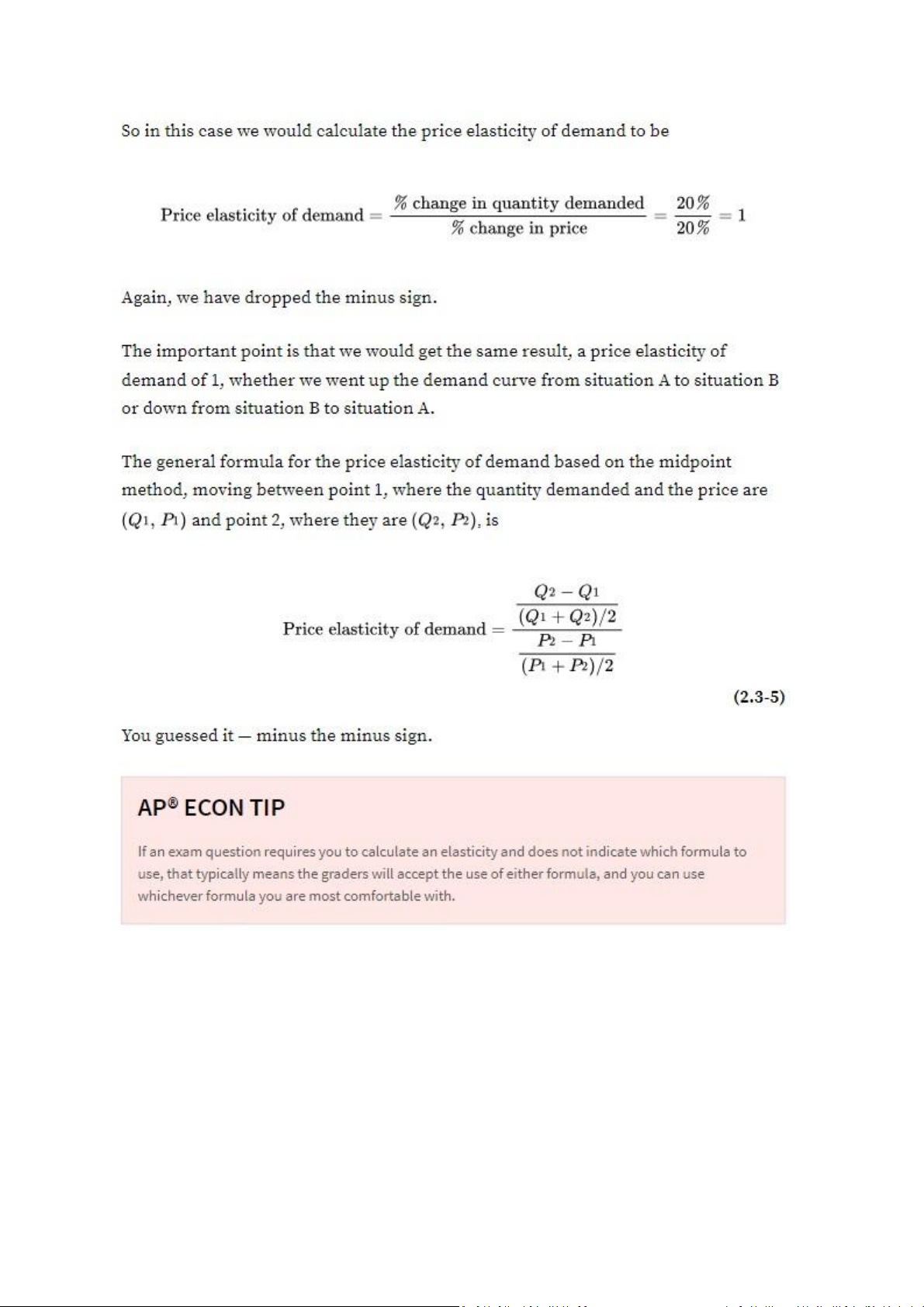
Using the midpoint method, we calculate the percentage change by dividing the change in a variable
by the average, or midpoint, of the initial and final values of that variable. So the average value of a variable, X, is defined as lOMoAR cPSD| 47882337 lOMoAR cPSD| 47882337 Elasticity Estimates
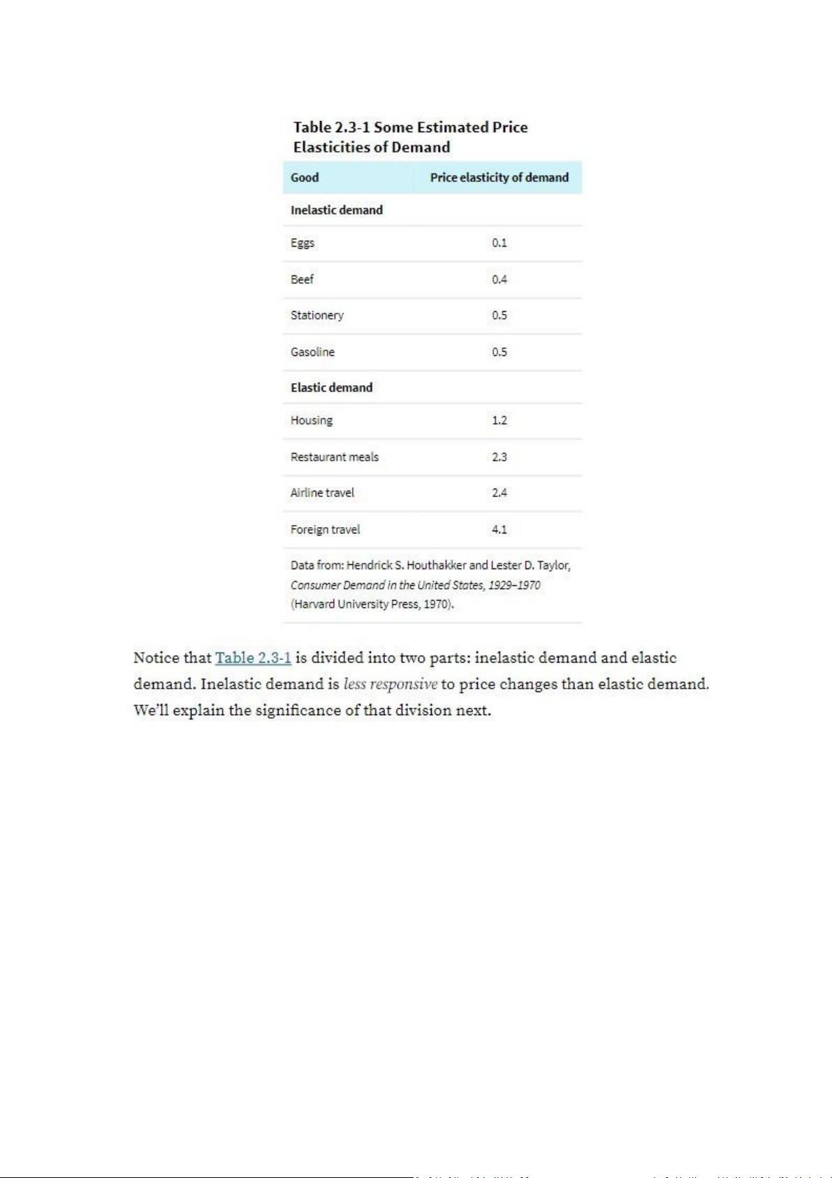
In 1970, economists Hendrik S. Houthakker and Lester D. Taylor published a comprehensive study
that estimated the price elasticities of demand for a wide variety of goods. Some of their results are
summarized in Table 2.3-1. These estimates show a wide range of price elasticities. There are some
goods, such as eggs, for which demand hardly responds at all to changes in the price; there are other
goods, most notably foreign travel, for which the quantity demanded is very sensitive to the price. lOMoAR cPSD| 47882337
What the Price Elasticity of Demand Tells Us
Well into the coronavirus pandemic, Pfizer-BioNTech raised the price of its COVID-19 vaccine by
about 25% in some countries because the price elasticity of demand was low. But what does that
mean? How low does a price elasticity have to be for it to be classified as low? How high does it have
to be for it to be considered high? And what determines whether the price elasticity of demand is
high or low? To answer these questions, we need to look more deeply at the price elasticity of demand. How Elastic Is Elastic?
As a first step toward classifying price elasticities of demand, let’s look at two extreme cases. First,
consider the demand for a good when people pay no attention to its price. Suppose, for example, lOMoAR cPSD| 47882337
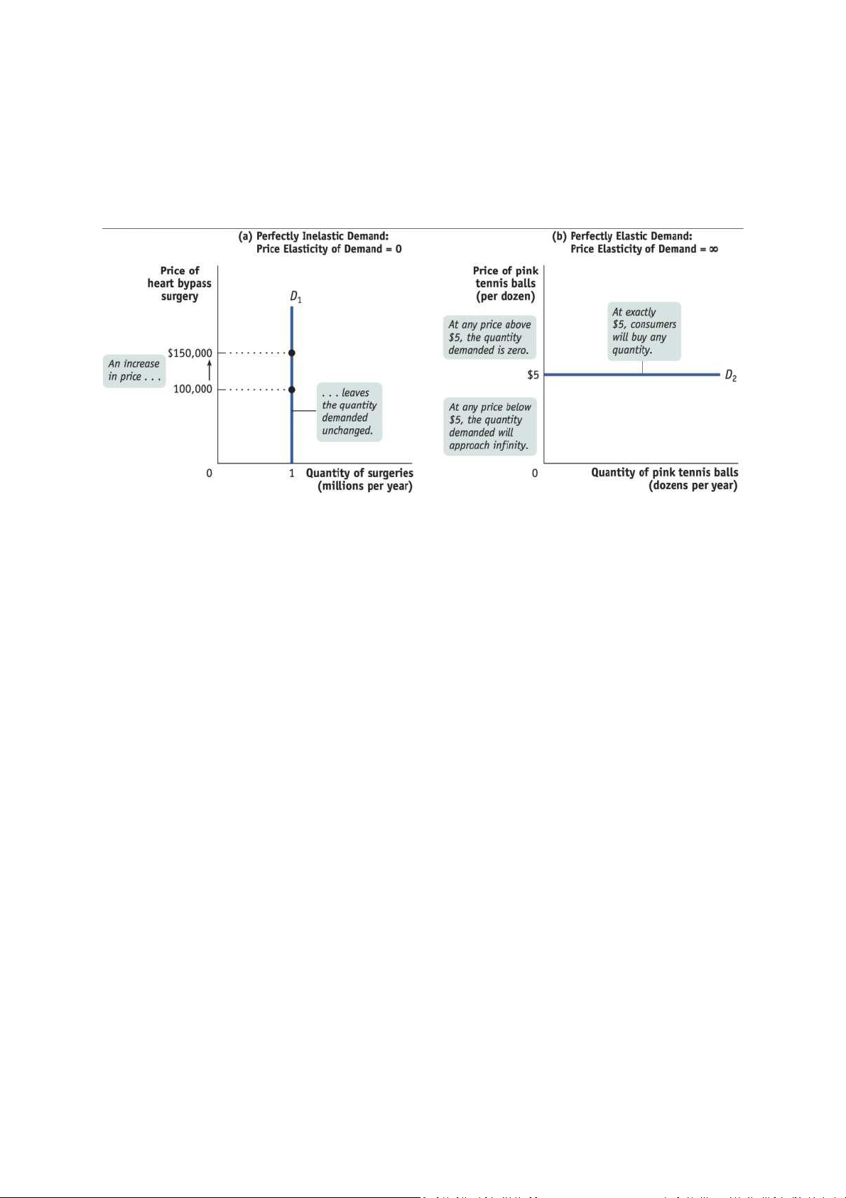
that consumers would buy 1 million heart bypass surgeries per year regardless of the price. If that
were true, the demand curve for these surgeries would look like the curve shown in panel (a) of
Figure 2.3-2: it would be a vertical line at 1 million heart bypass surgeries. Since the percentage
change in the quantity demanded is zero for any change in the price, the price elasticity of demand
in this case is zero. The case of a zero price elasticity of demand is known as perfectly inelastic demand. perfectly inelastic
Demand is perfectly inelastic when the quantity demanded does not respond at all to changes in the
price. When demand is perfectly inelastic, the demand curve is a vertical line.
The opposite extreme occurs when even a tiny rise in the price will cause the quantity demanded to
drop to zero or when even a tiny fall in the price will cause the quantity demanded to get extremely
large. Panel (b) of Figure 2.3-2 shows the case of pink tennis balls; we suppose that tennis players
don’t have a color preference, and that other tennis ball colors, such as neon green and vivid yellow,
are available at $5 per dozen balls. In this case, consumers will buy no pink tennis balls if they cost
more than $5 per dozen. But if pink tennis balls cost less than $5 per dozen, consumers will buy no
other color. The demand curve will therefore be a horizontal line at a price of $5 per dozen. If the
price falls from above $5 to below $5, the quantity demanded will rise from zero to a number
approaching infinity. So a horizontal demand curve implies an infinite price elasticity of demand.
When the price elasticity of demand is infinite, economists say that demand is perfectly elastic. perfectly elastic
Demand is perfectly elastic when any price increase will cause the quantity demanded to drop to
zero. When demand is perfectly elastic, the demand curve is a horizontal line.
The price elasticity of demand for the vast majority of goods is somewhere between these two
extreme cases. Economists use one level of magnitude for classifying these intermediate cases: they
ask whether the price elasticity of demand is greater or less than 1. When the price elasticity of
demand is greater than 1, economists say that demand is elastic. When the price elasticity of
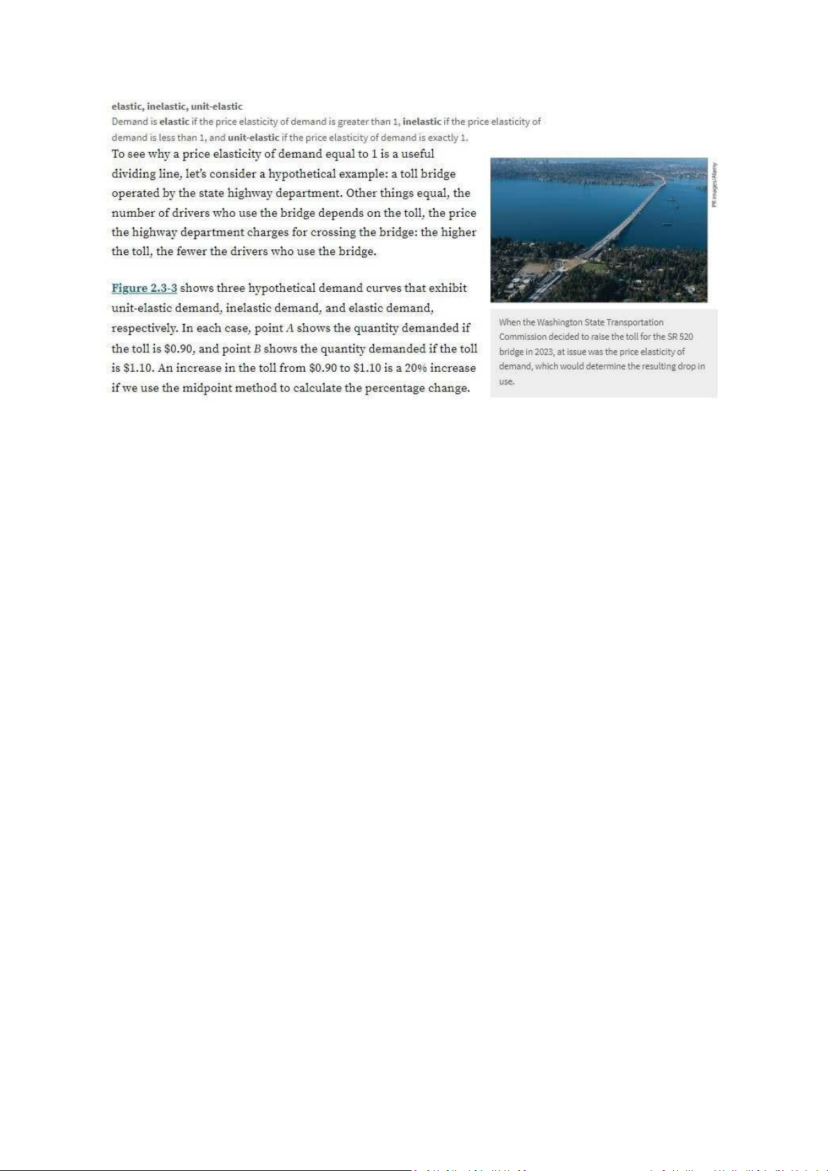
demand is less than 1, they say that demand is inelastic. The borderline case is unit-elastic demand,
where the price elasticity of demand is — surprise — exactly 1. lOMoAR cPSD| 47882337 lOMoAR cPSD| 47882337 lOMoAR cPSD| 47882337 lOMoAR cPSD| 47882337 lOMoAR cPSD| 47882337 lOMoAR cPSD| 47882337 lOMoAR cPSD| 47882337 lOMoAR cPSD| 47882337
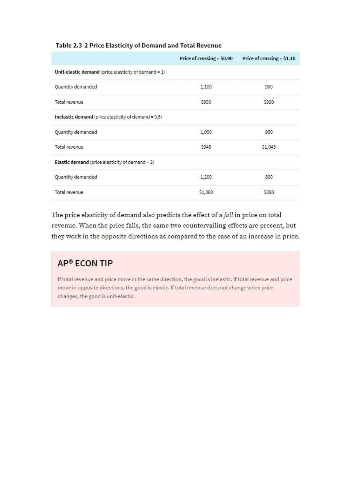
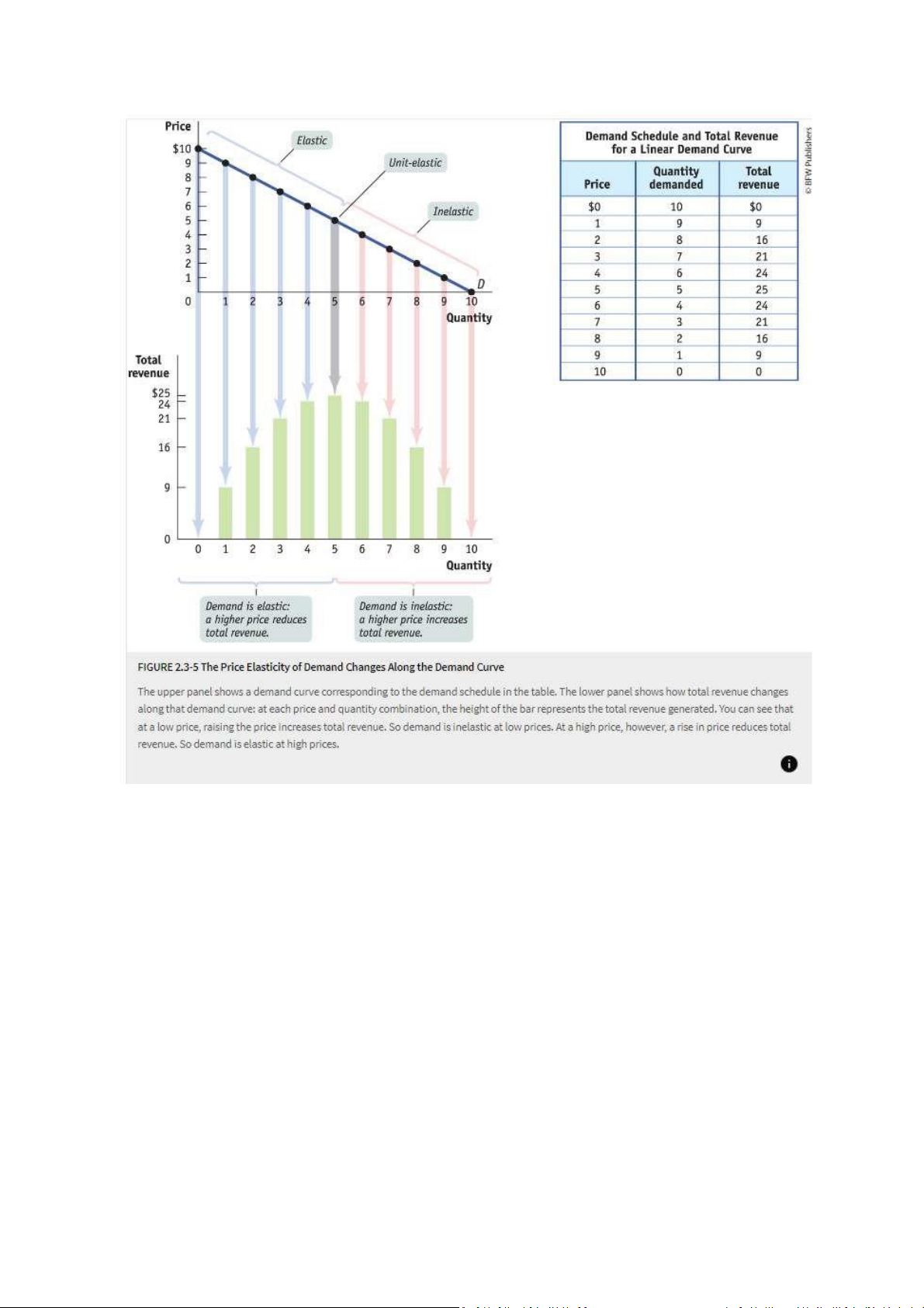
In Figure 2.3-5, you can see that when the price is low, raising the price increases total revenue:
starting at a price of $1, raising the price to $2 increases total revenue from $9 to $16. This means
that when the price is low, demand is inelastic. Moreover, you can see that demand is inelastic on
the entire section of the demand curve where the price is below $5. AP® ECON TIP
For a straight, downward-sloping demand curve, the upper left segment of the demand curve is
elastic and the bottom right segment is inelastic.
When the price is high, however, raising it further reduces total revenue: starting at a price of $8, for
example, raising the price to $9 reduces total revenue from $16 to $9. This means that when the
price is high, demand is elastic. Furthermore, you can see that demand is elastic over the section of
the demand curve where the price exceeds $5. lOMoAR cPSD| 47882337
For the vast majority of goods, the price elasticity of demand changes along the demand curve. So
whenever you measure a good’s elasticity, you are really measuring it at a particular point or section of the good’s demand curve.
What Factors Determine the Price Elasticity of Demand?
Pfizer-BioNTech was able to significantly raise its price for COVID-19 vaccines for several important
reasons: there were few substitutes, the price was a small fraction of the typical consumer’s income,
and many people considered them a medical necessity. Over time, some people were able to find
providers of alternative vaccines with lower prices. This experience illustrates the four main factors
that determine elasticity: whether close substitutes are available, the share of income a consumer
spends on the good, whether the good is a necessity or a luxury, and how much time has elapsed
since the price change. Let’s look at each of these factors in detail.
Whether Close Substitutes Are Available
The price elasticity of demand tends to be high if there are other goods that consumers regard as
similar and would be willing to consume instead. The price elasticity of demand tends to be low if
there are no close substitutes.
Share of Income Spent on the Good
The price elasticity of demand tends to be low when spending on a good accounts for a small share
of a consumer’s income. In that case, a significant change in the price of the good has little impact on
how much the consumer spends. In contrast, when a good accounts for a significant share of a
consumer’s spending, the consumer is likely to be very responsive to a change in price. In this case,
the price elasticity of demand is high.
Whether the Good Is a Necessity or a Luxury
The price elasticity of demand tends to be low if a good is something you must have, like a life-saving
medicine, or something you feel like you must have due to an addiction. The price elasticity of
demand tends to be high if the good is a luxury — something you can easily live without. Time
In general, the price elasticity of demand tends to increase as consumers have more time to adjust to
a price change. This means that the long-run price elasticity of demand is often higher than the short-run elasticity. AP® ECON TIP
Use the mnemonic SPLAT to help remember that the determinants of price elasticity of demand are:
Substitutes, Proportion of income, Luxury or necessity, Addictive or habit forming, and Time. lOMoAR cPSD| 47882337
A good illustration of the effect of time on the elasticity of demand is drawn from dramatic increases
in gasoline prices, which occurred in the United States in 2011 and 2021. Initially, consumption fell
very little because there were no close substitutes for gasoline and because people needed to drive
their cars to carry out the ordinary tasks of life. Over time, however, Americans changed their
carbuying and driving habits in ways that enabled them to gradually reduce their gasoline
consumption. Within two years of the 2011 increase, the average household used 19% less gasoline,
and the average vehicle used 14% less gasoline than they had a decade earlier, confirming that the
long-run price elasticity of demand for gasoline was indeed much higher than the short-run elasticity.
The 2021 increase was followed by burgeoning interest in electric vehicles.