Chapter 3: Algorithm Analysis in Data Structures and Algorithms Môn Câu trúc dữ liệu giải thuật | Trường Đại học Công nghiệp Thành phố Hồ Chí Minh
In a classic story, the famous mathematician Archimedes was asked to deter-mine if a golden crown commissioned by the king was indeed pure gold, and notpart silver, as an informant had claimed. Tài liệu gồm 39 trang, giúp các bạn tham khảo, ôn tập và đạt kết quả cao. Mình bạn đọc đón xem!
Môn: Câu trúc dữ liệu giải thuật (422000161) 12 tài liệu
Trường: Trường Đại học Công nghiệp Thành phố Hồ Chí Minh 776 tài liệu
Tác giả:


Preview text:
Chapter 3 Algorithm Analysis Contents 3.1
Experimental Studies ........................................................................... 111
3.1.1 Moving Beyond Experimental Analysis...................................... 113 3.2
The Seven Functions Used in This Book........................................ 115
3.2.1 Comparing Growth Rates ............................................................ 122 3.3
Asymptotic Analysis ............................................................................. 123
3.3.1 The “Big-Oh” Notation .............................................................. 123
3.3.2 Comparative Analysis .................................................................. 128
3.3.3 Examples of Algorithm Analysis ................................................. 130 3.4
Simple Justification Techniques........................................................ 137
3.4.1 By Example .................................................................................. 137
3.4.2 The “Contra” Attack ................................................................... 137
3.4.3 Induction and Loop Invariants ................................................... 138 3.5
Exercises ................................................................................................. 141 110
Chapter 3. Algorithm Analysis
In a classic story, the famous mathematician Archimedes was asked to deter-
mine if a golden crown commissioned by the king was indeed pure gold, and not
part silver, as an informant had claimed. Archimedes discovered a way to perform
this analysis while stepping into a bath. He noted that water spilled out of the bath
in proportion to the amount of him that went in. Realizing the implications of this
fact, he immediately got out of the bath and ran naked through the city shouting,
“Eureka, eureka!” for he had discovered an analysis tool (displacement), which,
when combined with a simple scale, could determine if the king’s new crown was
good or not. That is, Archimedes could dip the crown and an equal-weight amount
of gold into a bowl of water to see if they both displaced the same amount. This
discovery was unfortunate for the goldsmith, however, for when Archimedes did
his analysis, the crown displaced more water than an equal-weight lump of pure
gold, indicating that the crown was not, in fact, pure gold.
In this book, we are interested in the design of “good” data structures and algo-
rithms. Simply put, a data structure is a systematic way of organizing and access-
ing data, and an algorithm is a step-by-step procedure for performing some task in
a finite amount of time. These concepts are central to computing, but to be able to
classify some data structures and algorithms as “good,” we must have precise ways of analyzing them.
The primary analysis tool we will use in this book involves characterizing the
running times of algorithms and data structure operations, with space usage also
being of interest. Running time is a natural measure of “goodness,” since time is a
precious resource—computer solutions should run as fast as possible. In general,
the running time of an algorithm or data structure operation increases with the input
size, although it may also vary for different inputs of the same size. Also, the run-
ning time is affected by the hardware environment (e.g., the processor, clock rate,
memory, disk) and software environment (e.g., the operating system, programming
language) in which the algorithm is implemented and executed. All other factors
being equal, the running time of the same algorithm on the same input data will be
smaller if the computer has, say, a much faster processor or if the implementation
is done in a program compiled into native machine code instead of an interpreted
implementation. We begin this chapter by discussing tools for performing exper-
imental studies, yet also limitations to the use of experiments as a primary means
for evaluating algorithm efficiency.
Focusing on running time as a primary measure of goodness requires that we be
able to use a few mathematical tools. In spite of the possible variations that come
from different environmental factors, we would like to focus on the relationship
between the running time of an algorithm and the size of its input. We are interested
in characterizing an algorithm’s running time as a function of the input size. But
what is the proper way of measuring it? In this chapter, we “roll up our sleeves”
and develop a mathematical way of analyzing algorithms.
3.1. Experimental Studies 111 3.1 Experimental Studies
If an algorithm has been implemented, we can study its running time by executin g
it on various test inputs and recording the time spent during each execution. A
simple approach for doing this in Python is by using the time function of the time
module. This function reports the number of seconds, or fractions thereof, that have
elapsed since a benchmark time known as the epoch. The choice of the epoch is
not significant to our goal, as we can determine the elapsed time by recording the
time just before the algorithm and the time just after the algorithm, and computin g their difference, as follows: from time import time start time = time( ) # record the starting time run algorithm end time = time( ) # record the ending time
elapsed = end time − start time # compute the elapsed time
We will demonstrate use of this approach, in Chapter 5, to gather experimental data
on the efficiency of Python’s list class. An elapsed time measured in this fashion
is a decent reflection of the algorithm efficiency, but it is by no means perfect. The
time function measures relative to what is known as the “wall clock.” Because
many processes share use of a computer’s central processing unit (or CPU), the
elapsed time will depend on what other processes are running on the computer
when the test is performed. A fairer metric is the number of CPU cycles that are
used by the algorithm. This can be determined using the clock function of the time
module, but even this measure might not be consistent if repeating the identica l
algorithm on the identical input, and its granularity will depend upon the computer
system. Python includes a more advanced module, named timeit, to help automate
such evaluations with repetition to account for such variance among trials.
Because we are interested in the general dependence of running time on the size
and structure of the input, we should perform independent experiments on many
different test inputs of various sizes. We can then visualize the results by plotting
the performance of each run of the algorithm as a point with x-coordinate equal to
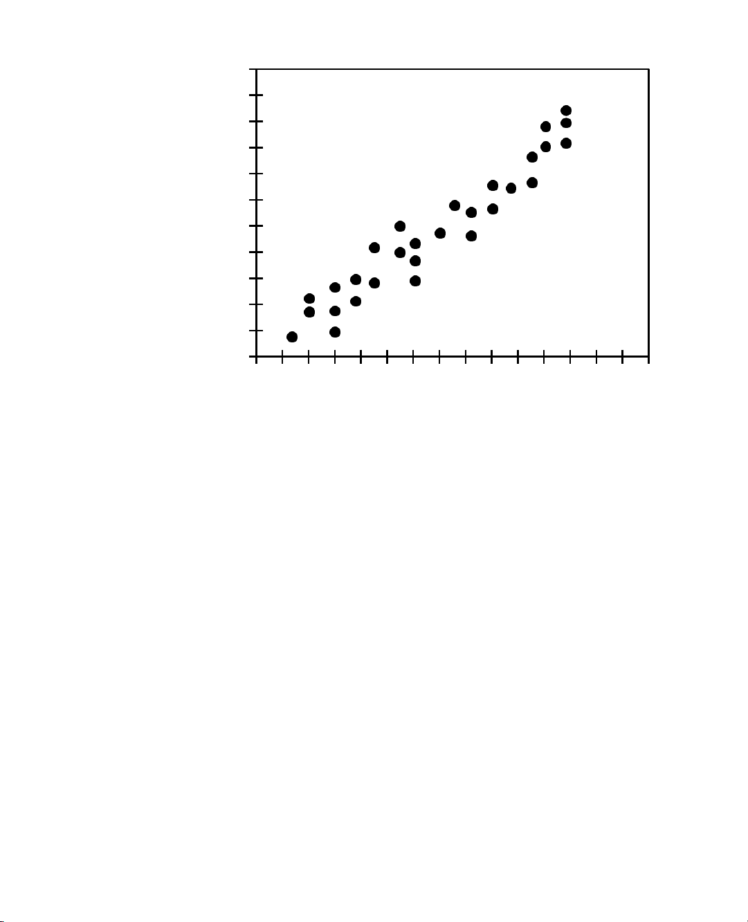
the input size, n, and y-coordinate equal to the running time, t. Figure 3.1 displays
such hypothetical data. This visualization may provide some intuition regardin g
the relationship between problem size and execution time for the algorithm. This
may lead to a statistical analysis that seeks to fit the best function of the input size
to the experimental data. To be meaningful, this analysis requires that we choose
good sample inputs and test enough of them to be able to make sound statistica l
claims about the algorithm’s running time. 112
Chapter 3. Algorithm Analysis 500 400 ) s m( e 300 mi T g nin 200 n u R 100 0 0 5000 10000 15000 Input Size
Figure 3.1: Results of an experimental study on the running time of an algorithm.
A dot with coordinates (n,t) indicates that on an input of size n, the running time
of the algorithm was measured as t milliseconds (ms).
Challenges of Experimental Analysis
While experimental studies of running times are valuable, especially when fine-
tuning production-quality code, there are three major limitations to their use for algorithm analysis:
• Experimental running times of two algorithms are difficult to directly com-
pare unless the experiments are performed in the same hardware and software environments.
• Experiments can be done only on a limited set of test inputs; hence, they
leave out the running times of inputs not included in the experiment (and
these inputs may be important).
• An algorithm must be fully implemented in order to execute it to study its running time experimentally.
This last requirement is the most serious drawback to the use of experimental stud-
ies. At early stages of design, when considering a choice of data structures or
algorithms, it would be foolish to spend a significant amount of time implementing
an approach that could easily be deemed inferior by a higher-level analysis.
3.1. Experimental Studies 113
3.1.1 Moving Beyond Experimental Analysis
Our goal is to develop an approach to analyzing the efficiency of algorithms that:
1. Allows us to evaluate the relative efficiency of any two algorithms in a way
that is independent of the hardware and software environment.
2. Is performed by studying a high-level description of the algorithm without need for implementation.
3. Takes into account all possible inputs. Counting Primitive Operations
To analyze the running time of an algorithm without performing experiments, we
perform an analysis directly on a high-level description of the algorithm (either in
the form of an actual code fragment, or language-independent pseudo-code). We
define a set of primitive operations such as the following:
• Assigning an identifier to an object
• Determining the object associated with an identifier
• Performing an arithmetic operation (for example, adding two numbers) • Comparing two numbers
• Accessing a single element of a Python list by index
• Calling a function (excluding operations executed within the function)
• Returning from a function.
Formally, a primitive operation corresponds to a low-level instruction with an exe-
cution time that is constant. Ideally, this might be the type of basic operation that is
executed by the hardware, although many of our primitive operations may be trans-
lated to a small number of instructions. Instead of trying to determine the specific
execution time of each primitive operation, we will simply count how many prim-
itive operations are executed, and use this number t as a measure of the runnin g time of the algorithm.
This operation count will correlate to an actual running time in a specific com-
puter, for each primitive operation corresponds to a constant number of instructions,
and there are only a fixed number of primitive operations. The implicit assumption
in this approach is that the running times of different primitive operations will be
fairly similar. Thus, the number, t, of primitive operations an algorithm performs
will be proportional to the actual running time of that algorithm.
Measuring Operations as a Function of Input Size
To capture the order of growth of an algorithm’s running time, we will associate,
with each algorithm, a function f (n) that characterizes the number of primitive
operations that are performed as a function of the input size n. Section 3.2 will in-
troduce the seven most common functions that arise, and Section 3.3 will introduce
a mathematical framework for comparing functions to each other. 114
Chapter 3. Algorithm Analysis
Focusing on the Worst-Case Input
An algorithm may run faster on some inputs than it does on others of the same size.
Thus, we may wish to express the running time of an algorithm as the function of
the input size obtained by taking the average over all possible inputs of the same
size. Unfortunately, such an average-case analysis is typically quite challenging.
It requires us to define a probability distribution on the set of inputs, which is often
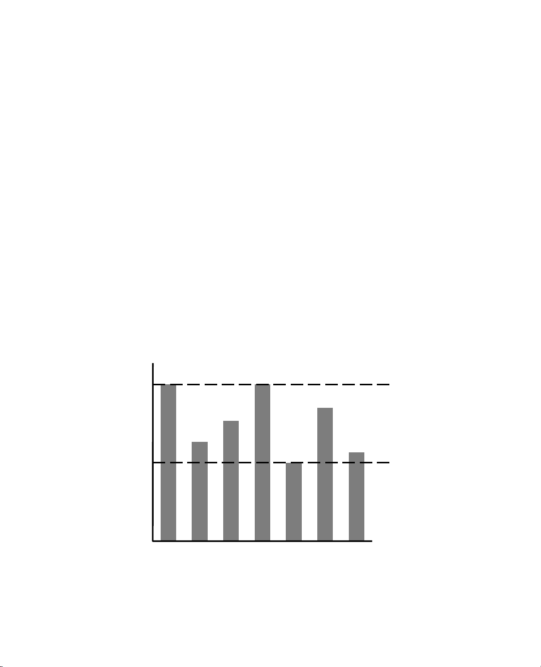
a difficult task. Figure 3.2 schematically shows how, depending on the input distri-
bution, the running time of an algorithm can be anywhere between the worst-case
time and the best-case time. For example, what if inputs are really only of types “A” or “D”?
An average-case analysis usually requires that we calculate expected runnin g
times based on a given input distribution, which usually involves sophisticated
probability theory. Therefore, for the remainder of this book, unless we specify
otherwise, we will characterize running times in terms of the worst case, as a func-
tion of the input size, n, of the algorithm.
Worst-case analysis is much easier than average-case analysis, as it requires
only the ability to identify the worst-case input, which is often simple. Also, this
approach typically leads to better algorithms. Making the standard of success for an
algorithm to perform well in the worst case necessarily requires that it will do well
on every input. That is, designing for the worst case leads to stronger algorithmic
“muscles,” much like a track star who always practices by running up an incline. 5 ms worst-c ase time ) s 4 ms m( average-case time? e mi T 3 ms g n i best-case time n n u 2 ms R 1 ms A B C D E F G Input Instance
Figure 3.2: The difference between best-case and worst-case time. Each bar repre-
sents the running time of some algorithm on a different possible input.
3.2. The Seven Functions Used in This Book 115
3.2 The Seven Functions Used in This Book
In this section, we briefly discuss the seven most important functions used in the
analysis of algorithms. We will use only these seven simple functions for almost
all the analysis we do in this book. In fact, a section that uses a function other
than one of these seven will be marked with a star ( ) to indicate that it is optional.
In addition to these seven fundamental functions, Appendix B contains a list of
other useful mathematical facts that apply in the analysis of data structures and algorithms. The Constant Function
The simplest function we can think of is the constant function. This is the function,
f (n) = c,
for some fixed constant c, such as c = 5, c = 27, or c = 210. That is, for any
argument n, the constant function f (n) assigns the value c. In other words, it does
not matter what the value of n is; f (n) will always be equal to the constant value c.
Because we are most interested in integer functions, the most fundamental con-
stant function is g(n) = 1, and this is the typical constant function we use in this
book. Note that any other constant function, f (n) = c, can be written as a constant
c times g(n). That is, f (n) = cg(n) in this case.
As simple as it is, the constant function is useful in algorithm analysis, because
it characterizes the number of steps needed to do a basic operation on a computer,
like adding two numbers, assigning a value to some variable, or comparing two numbers. The Logarithm Function
One of the interesting and sometimes even surprising aspects of the analysis of
data structures and algorithms is the ubiquitous presence of the logarithm function,
f (n) = logb n, for some constant b > 1. This function is defined as follows:
x = logb n if and only if bx = n.
By definition, logb 1 = 0. The value b is known as the base of the logarithm.
The most common base for the logarithm function in computer science is 2,
as computers store integers in binary, and because a common operation in many
algorithms is to repeatedly divide an input in half. In fact, this base is so common
that we will typically omit it from the notation when it is 2. That is, for us, log n = log2 n. 116
Chapter 3. Algorithm Analysis
We note that most handheld calculators have a button marked LOG, but this is
typically for calculating the logarithm base-10, not base-two.
Computing the logarithm function exactly for any integer n involves the use
of calculus, but we can use an approximation that is good enough for our pur-
poses without calculus. In particular, we can easily compute the smallest integer
greater than or equal to logb n (its so-called ceiling, [logb n|). For positive integer,
n, this value is equal to the number of times we can divide n by b before we get
a number less than or equal to 1. For example, the evaluation of [log3 27| is 3,
because ((27/3)/3)/3 = 1. Likewise, [log4 64| is 3, because ((64/4)/4)/4 = 1,
and [log2 12| is 4, because (((12/2)/2)/2)/2 = 0.75 ≤ 1.
The following proposition describes several important identities that involve
logarithms for any base greater than 1.
Proposition 3.1 (Logarithm Rules): Given real numbers a > 0, b > 1, c > 0 and d > 1, we have: 1. log (
b ac) = logb a + logb c 2. log (
b a/c) = logb a − logb c 3. log (
b ac) = c logb a
4. logb a = logd a/ logd b
5. blogd a = alogd b
By convention, the unparenthesized notation log nc denotes the value log(nc).
We use a notational shorthand, logc n, to denote the quantity, (log n)c, in which the
result of the logarithm is raised to a power.
The above identities can be derived from converse rules for exponentiation that
we will present on page 121. We illustrate these identities with a few examples.
Example 3.2: We demonstrate below some interesting applications of the loga-
rithm rules from Proposition 3.1 (using the usual convention that the base of a
logarithm is 2 if it is omitted).
• log(2n) = log 2 + log n = 1 + log n, by rule 1
• log(n/2) = log n − log 2 = log n − 1, by rule 2
• log n3 = 3 log n, by rule 3
• log 2n = n log 2 = n · 1 = n, by rule 3
• log4 n = (log n)/ log 4 = (log n)/2, by rule 4
• 2logn = nlog2 = n1 = n, by rule 5.
As a practical matter, we note that rule 4 gives us a way to compute the base-two
logarithm on a calculator that has a base-10 logarithm button, LOG, for
log2 n = LOG n / LOG 2.
3.2. The Seven Functions Used in This Book 117 The Linear Function
Another simple yet important function is the linear function,
f (n) = n.
That is, given an input value n, the linear function f assigns the value n itself.
This function arises in algorithm analysis any time we have to do a single basic
operation for each of n elements. For example, comparing a number x to each
element of a sequence of size n will require n comparisons. The linear function
also represents the best running time we can hope to achieve for any algorithm that
processes each of n objects that are not already in the computer’s memory, because
reading in the n objects already requires n operations.
The N-Log-N Function
The next function we discuss in this section is the n-log-n function,
f (n) = n log n,
that is, the function that assigns to an input n the value of n times the logarithm
base-two of n. This function grows a little more rapidly than the linear function and
a lot less rapidly than the quadratic function; therefore, we would greatly prefer an
algorithm with a running time that is proportional to n log n, than one with quadratic
running time. We will see several important algorithms that exhibit a running time
proportional to the n-log-n function. For example, the fastest possible algorithms
for sorting n arbitrary values require time proportional to n log n. The Quadratic Function
Another function that appears often in algorithm analysis is the quadratic function,
f (n) = n2.
That is, given an input value n, the function f assigns the product of n with itself
(in other words, “n squared”).
The main reason why the quadratic function appears in the analysis of algo -
rithms is that there are many algorithms that have nested loops, where the inner
loop performs a linear number of operations and the outer loop is performed a
linear number of times. Thus, in such cases, the algorithm performs n · n = n2 operations. 118
Chapter 3. Algorithm Analysis
Nested Loops and the Quadratic Function
The quadratic function can also arise in the context of nested loops where the first
iteration of a loop uses one operation, the second uses two operations, the third uses
three operations, and so on. That is, the number of operations is
1 + 2 + 3 + · · · + (n − 2) + (n − 1) + n.
In other words, this is the total number of operations that will be performed by the
nested loop if the number of operations performed inside the loop increases by one
with each iteration of the outer loop. This quantity also has an interesting history.
In 1787, a German schoolteacher decided to keep his 9- and 10-year-old pupils
occupied by adding up the integers from 1 to 100. But almost immediately one
of the children claimed to have the answer! The teacher was suspicious, for the
student had only the answer on his slate. But the answer, 5050, was correct and the
student, Carl Gauss, grew up to be one of the greatest mathematicians of his time.
We presume that young Gauss used the following identity.
Proposition 3.3: For any integer n ≥ 1, we have: n(n + 1)
1 + 2 + 3 + · · · + (n − 2) + (n − 1) + n = . 2
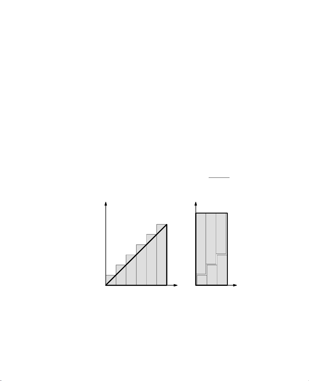
We give two “visual” justifications of Proposition 3.3 in Figure 3.3. n+1 n n ... ... 3 3 2 2 1 1 0 1 2 3 n 0 1 2 n/2 (a) (b)
Figure 3.3: Visual justifications of Proposition 3.3. Both illustrations visualize the
identity in terms of the total area covered by n unit-width rectangles with heights
1, 2, . . . , n. In (a), the rectangles are shown to cover a big triangle of area n2/2 (base
n and height n) plus n small triangles of area 1/2 each (base 1 and height 1). In
(b) , which applies only when n is even, the rectangles are shown to cover a big
rectangle of base n/2 and height n + 1.
3.2. The Seven Functions Used in This Book 119
The lesson to be learned from Proposition 3.3 is that if we perform an algorithm
with nested loops such that the operations in the inner loop increase by one each
time, then the total number of operations is quadratic in the number of times, n,
we perform the outer loop. To be fair, the number of operations is n2/2 + n/2,
and so this is just over half the number of operations than an algorithm that uses n
operations each time the inner loop is performed. But the order of growth is still quadratic in n.
The Cubic Function and Other Polynomials
Continuing our discussion of functions that are powers of the input, we consider
the cubic function,
f (n) = n3,
which assigns to an input value n the product of n with itself three times. This func-
tion appears less frequently in the context of algorithm analysis than the constant,
linear, and quadratic functions previously mentioned, but it does appear from time to time. Polynomials
Most of the functions we have listed so far can each be viewed as being part of a
larger class of functions, the polynomials. A polynomial function has the form,
f (n) = a0 + a1n + a2n2 + a3n3 + · · · + adnd, where a , , . . . , 0 a1
ad are constants, called the coefficients of the polynomial, and
ad /= 0. Integer d, which indicates the highest power in the polynomial, is called
the degree of the polynomial.
For example, the following functions are all polynomials:
• f (n) = 2 + 5n + n2
• f (n) = 1 + n3 • f (n) = 1
• f (n) = n
• f (n) = n2
Therefore, we could argue that this book presents just four important functions used
in algorithm analysis, but we will stick to saying that there are seven, since the con-
stant, linear, and quadratic functions are too important to be lumped in with other
polynomials. Running times that are polynomials with small degree are generally
better than polynomial running times with larger degree. 120
Chapter 3. Algorithm Analysis Summations
A notation that appears again and again in the analysis of data structures and algo-
rithms is the summation, which is defined as follows: b
f (i) = f (a) + f (a + 1) + f (a + 2) + · · · + f (b), i=a
where a and b are integers and a ≤ b. Summations arise in data structure and algo-
rithm analysis because the running times of loops naturally give rise to summations.
Using a summation, we can rewrite the formula of Proposition 3.3 as n n(n + 1) i = . 2 i=1
Likewise, we can write a polynomial f (n) of degree d with coefficients a , . . . , 0 ad as d
f (n) = aini. i=0
Thus, the summation notation gives us a shorthand way of expressing sums of in-
creasing terms that have a regular structure. The Exponential Function
Another function used in the analysis of algorithms is the exponential function,
f (n) = bn,
where b is a positive constant, called the base, and the argument n is the exponent.
That is, function f (n) assigns to the input argument n the value obtained by mul-
tiplying the base b by itself n times. As was the case with the logarithm function,
the most common base for the exponential function in algorithm analysis is b = 2.
For example, an integer word containing n bits can represent all the nonnegative
integers less than 2n. If we have a loop that starts by performing one operation
and then doubles the number of operations performed with each iteration, then the
number of operations performed in the nth iteration is 2n.
We sometimes have other exponents besides n, however; hence, it is useful
for us to know a few handy rules for working with exponents. In particular, the
following exponent rules are quite helpful.
3.2. The Seven Functions Used in This Book 121
Proposition 3.4 (Exponent Rules): Given positive integers a, b, and c, we have
1. (ba)c = bac
2. babc = ba+c
3. ba/bc = ba−c
For example, we have the following:
• 256 = 162 = (24)2 = 24·2 = 28 = 256 (Exponent Rule 1)
• 243 = 35 = 32+3 = 3233 = 9 · 27 = 243 (Exponent Rule 2)
• 16 = 1024/64 = 210/26 = 210−6 = 24 = 16 (Exponent Rule 3)
We can extend the exponential function to exponents that are fractions or real
numbers and to negative exponents, as follows. Given a positive integer k, we de-
fine b1/k to be kth root of b, that is, the number r such that rk = b. For example,
251/2 = 5, since 52 = 25. Likewise, 271/3 = 3 and 161/4 = 2. This approach al-
lows us to define any power whose exponent can be expressed as a fraction, for
ba/c = (ba)1/c, by Exponent Rule 1. For example, 93/2 = (93)1/2 = 7291/2 = 27.
Thus, ba/c is really just the cth root of the integral exponent ba.
We can further extend the exponential function to define bx for any real number
x, by computing a series of numbers of the form ba/c for fractions a/c that get pro-
gressively closer and closer to x. Any real number x can be approximated arbitrarily
closely by a fraction a/c; hence, we can use the fraction a/c as the exponent of b
to get arbitrarily close to bx. For example, the number 2 is well defined. Finally,
given a negative exponent d, we define bd = 1/b−d, which corresponds to applying
Exponent Rule 3 with a = 0 and c = −d. For example, 2−3 = 1/23 = 1/8. Geometric Sums
Suppose we have a loop for which each iteration takes a multiplicative factor longer
than the previous one. This loop can be analyzed using the following proposition.
Proposition 3.5: For any integer n ≥ 0 and any real number a such that a > 0 and a / = 1, consider the summation n
ai = 1 + a + a2 + · · · + an i=0
(remembering that a0 = 1 if a > 0). This summation is equal to an+1 − 1 . a − 1
Summations as shown in Proposition 3.5 are called geometric summations, be-
cause each term is geometrically larger than the previous one if a > 1. For example,
everyone working in computing should know that
1 + 2 + 4 + 8 + · · · + 2n−1 = 2n − 1,
for this is the largest integer that can be represented in binary notation using n bits. 122
Chapter 3. Algorithm Analysis 3.2.1 Comparing Growth Rates
To sum up, Table 3.1 shows, in order, each of the seven common functions used in algorithm analysis. constant logarithm linear
n-log-n quadratic cubic exponential 1 log n n n log n n2 n3 an
Table 3.1: Classes of functions. Here we assume that a > 1 is a constant.
Ideally, we would like data structure operations to run in times proportional
to the constant or logarithm function, and we would like our algorithms to run in
linear or n-log-n time. Algorithms with quadratic or cubic running times are less
practical, and algorithms with exponential running times are infeasible for all but
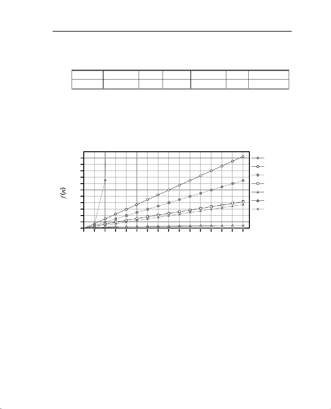
the smallest sized inputs. Plots of the seven functions are shown in Figure 3.4. 1044 Exponential 1040 Cubic 1036 1032 Quadratic 1028 N-Log-N 1024 Linear 1020 1016 Logarithmic 1012 Constant 108 104 100
100 101 102 103 104 105 106 107 108 109 1010 1011 1012 1013 1014 1015 n
Figure 3.4: Growth rates for the seven fundamental functions used in algorithm
analysis. We use base a = 2 for the exponential function. The functions are plotted
on a log-log chart, to compare the growth rates primarily as slopes. Even so, the
exponential function grows too fast to display all its values on the chart.
The Ceiling and Floor Functions
One additional comment concerning the functions above is in order. When dis-
cussing logarithms, we noted that the value is generally not an integer, yet the
running time of an algorithm is usually expressed by means of an integer quantity,
such as the number of operations performed. Thus, the analysis of an algorithm
may sometimes involve the use of the floor function and ceiling function, which
are defined respectively as follows:
• [x♩ = the largest integer less than or equal to x.
• [x| = the smallest integer greater than or equal to x.
3.3. Asymptotic Analysis 123 3.3 Asymptotic Analysis
In algorithm analysis, we focus on the growth rate of the running time as a function
of the input size n, taking a “big-picture” approach. For example, it is often enough
just to know that the running time of an algorithm grows proportionally to n.
We analyze algorithms using a mathematical notation for functions that disre-
gards constant factors. Namely, we characterize the running times of algorithms
by using functions that map the size of the input, n, to values that correspond to
the main factor that determines the growth rate in terms of n. This approach re-
flects that each basic step in a pseudo-code description or a high-level language
implementation may correspond to a small number of primitive operations. Thus,
we can perform an analysis of an algorithm by estimating the number of primitive
operations executed up to a constant factor, rather than getting bogged down in
language-specific or hardware-specific analysis of the exact number of operations that execute on the computer.
As a tangible example, we revisit the goal of finding the largest element of a
Python list; we first used this example when introducing for loops on page 21 of
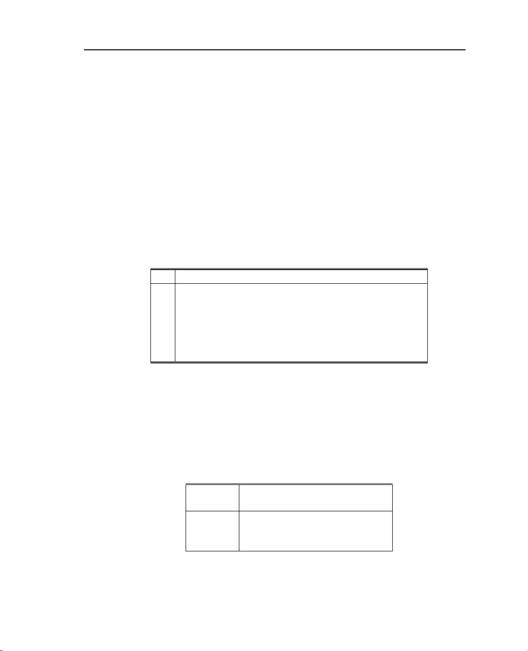
Section 1.4.2. Code Fragment 3.1 presents a function named find max for this task. 1 def find max(data): 2
”””Return the maximum element from a nonempty Python list.””” 3 biggest = data[0] # The initial value to beat 4 for val in data: # For each value: 5 if val > biggest
# if it is greater than the best so far, 6 biggest = val
# we have found a new best (so far) 7 return biggest
# When loop ends, biggest is the max
Code Fragment 3.1: A function that returns the maximum value of a Python list.
This is a classic example of an algorithm with a running time that grows pro-
portional to n, as the loop executes once for each data element, with some fixed
number of primitive operations executing for each pass. In the remainder of this
section, we provide a framework to formalize this claim.
3.3.1 The “Big-Oh” Notation
Let f (n) and g(n) be functions mapping positive integers to positive real numbers.
We say that f (n) is O(g(n)) if there is a real constant c > 0 and an integer constant n0 ≥ 1 such that
f (n) ≤ cg(n), for n ≥ n . 0
This definition is often referred to as the “big-Oh” notation, for it is sometimes pro-
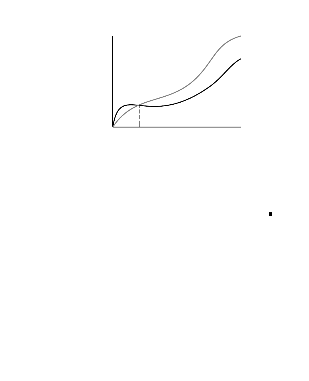
nounced as “ f (n) is big-Oh of g(n).” Figure 3.5 illustrates the general definition. 124
Chapter 3. Algorithm Analysis cg(n) e Tim f(n) Running n0 Input Size
Figure 3.5: Illustrating the “big-Oh” notation. The function f (n) is O(g(n)), since
f (n) ≤ c · g(n) when n ≥ n0.
Example 3.6: The function 8n + 5 is O(n).
Justification: By the big-Oh definition, we need to find a real constant c > 0 and
an integer constant n0 ≥ 1 such that 8n + 5 ≤ cn for every integer n ≥ n0. It is easy
to see that a possible choice is c = 9 and n0 = 5. Indeed, this is one of infinitely
many choices available because there is a trade-off between c and n0. For example,
we could rely on constants c = 13 and n0 = 1.
The big-Oh notation allows us to say that a function f (n) is “less than or equal
to” another function g(n) up to a constant factor and in the asymptotic sense as n
grows toward infinity. This ability comes from the fact that the definition uses “≤”
to compare f (n) to a g(n) times a constant, c, for the asymptotic cases when n ≥ n0.
However, it is considered poor taste to say “ f (n) ≤ O(g(n)),” since the big-Oh
already denotes the “less-than-or-equal-to” concept. Likewise, although common,
it is not fully correct to say “ f (n) = O(g(n)),” with the usual understanding of the
“=” relation, because there is no way to make sense of the symmetric statement,
“O(g(n)) = f (n).” It is best to say,
“ f (n) is O(g(n)).”
Alternatively, we can say “ f (n) is order of g(n).” For the more mathematically
inclined, it is also correct to say, “ f (n) ∈ O(g(n)),” for the big-Oh notation, techni-
cally speaking, denotes a whole collection of functions. In this book, we will stick
to presenting big-Oh statements as “ f (n) is O(g(n)).” Even with this interpretation,
there is considerable freedom in how we can use arithmetic operations with the big-
Oh notation, and with this freedom comes a certain amount of responsibility.
3.3. Asymptotic Analysis 125
Characterizing Running Times Using the Big-Oh Notation
The big-Oh notation is used widely to characterize running times and space bounds
in terms of some parameter n, which varies from problem to problem, but is always
defined as a chosen measure of the “size” of the problem. For example, if we
are interested in finding the largest element in a sequence, as with the find max
algorithm, we should let n denote the number of elements in that collection. Usin g
the big-Oh notation, we can write the following mathematically precise statement
on the running time of algorithm find max (Code Fragment 3.1) for any computer.
Proposition 3.7: The algorithm, find max, for computing the maximum element
of a list of n numbers, runs in O(n) time.
Justification: The initialization before the loop begins requires only a constant
number of primitive operations. Each iteration of the loop also requires only a con-
stant number of primitive operations, and the loop executes n times. Therefore,
we account for the number of primitive operations being c' + c'' · n for appropriate
constants c' and c'' that reflect, respectively, the work performed during initializa-
tion and the loop body. Because each primitive operation runs in constant time, we
have that the running time of algorithm find max on an input of size n is at most a
constant times n; that is, we conclude that the running time of algorithm find max is O(n).
Some Properties of the Big-Oh Notation
The big-Oh notation allows us to ignore constant factors and lower-order terms and
focus on the main components of a function that affect its growth.
Example 3.8: 5n4 + 3n3 + 2n2 + 4n + 1 is O(n4). Justification:
Note that 5n4 + 3n3 + 2n2 + 4n + 1 ≤ (5 + 3 + 2 + 4 + 1)n4 = cn4,
for c = 15, when n ≥ n0 = 1.
In fact, we can characterize the growth rate of any polynomial function.
Proposition 3.9: If f (n) is a polynomial of degree d, that is,
f (n) = a0 + a1n + · · · + adnd,
and ad > 0, then f (n) is O(nd). Justification:
Note that, for n ≥ 1, we have 1 ≤ n ≤ n2 ≤ · · · ≤ nd; hence, a
| + | | + | | + · · · + | |)
0 + a1n + a2n2 + · · · + adnd ≤ (|a0 a1 a2 ad nd.
We show that f (n) is O(nd) by defining c = |a | + | | + · · · + | | 0 a1 ad and n0 = 1. 126
Chapter 3. Algorithm Analysis
Thus, the highest-degree term in a polynomial is the term that determines the
asymptotic growth rate of that polynomial. We consider some additional properties
of the big-Oh notation in the exercises. Let us consider some further examples here,
focusing on combinations of the seven fundamental functions used in algorithm
design. We rely on the mathematical fact that log n ≤ n for n ≥ 1.
Example 3.10: 5n2 + 3n log n + 2n + 5 is O(n2). Justification:
5n2 + 3n log n + 2n + 5 ≤ (5 + 3 + 2 + 5)n2 = cn2, for c = 15, when n ≥ n0 = 1.
Example 3.11: 20n3 + 10n log n + 5 is O(n3). Justification:
20n3 + 10n log n + 5 ≤ 35n3, for n ≥ 1.
Example 3.12: 3 log n + 2 is O(log n). Justification:
3 log n + 2 ≤ 5 log n, for n ≥ 2. Note that log n is zero for n = 1.
That is why we use n ≥ n0 = 2 in this case.
Example 3.13: 2n+2 is O(2n). Justification:
2n+2 = 2n · 22 = 4 · 2n; hence, we can take c = 4 and n0 = 1 in this case.
Example 3.14: 2n + 100 log n is O(n). Justification:
2n + 100 log n ≤ 102n, for n ≥ n0 = 1; hence, we can take c = 102 in this case.
Characterizing Functions in Simplest Terms
In general, we should use the big-Oh notation to characterize a function as closely
as possible. While it is true that the function f (n) = 4n3 + 3n2 is O(n5) or even
O(n4), it is more accurate to say that f (n) is O(n3). Consider, by way of analogy,
a scenario where a hungry traveler driving along a long country road happens upon
a local farmer walking home from a market. If the traveler asks the farmer how
much longer he must drive before he can find some food, it may be truthful for the
farmer to say, “certainly no longer than 12 hours,” but it is much more accurate
(and helpful) for him to say, “you can find a market just a few minutes drive up this
road.” Thus, even with the big-Oh notation, we should strive as much as possible to tell the whole truth.
It is also considered poor taste to include constant factors and lower-order terms
in the big-Oh notation. For example, it is not fashionable to say that the function
2n2 is O(4n2 + 6n log n), although this is completely correct. We should strive
instead to describe the function in the big-Oh in simplest terms.
3.3. Asymptotic Analysis 127
The seven functions listed in Section 3.2 are the most common functions used
in conjunction with the big-Oh notation to characterize the running times and space
usage of algorithms. Indeed, we typically use the names of these functions to refer
to the running times of the algorithms they characterize. So, for example, we would
say that an algorithm that runs in worst-case time 4n2 + n log n is a quadratic-time
algorithm, since it runs in O(n2) time. Likewise, an algorithm running in time at
most 5n + 20 log n + 4 would be called a linear-time algorithm. Big-Omega
Just as the big-Oh notation provides an asymptotic way of saying that a function is
“less than or equal to” another function, the following notations provide an asymp-
totic way of saying that a function grows at a rate that is “greater than or equal to” that of another.
Let f (n) and g(n) be functions mapping positive integers to positive real num-
bers. We say that f (n) is (g(n)), pronounced “ f (n) is big-Omega of g(n),” if g(n)
is O( f (n)), that is, there is a real constant c > 0 and an integer constant n0 ≥ 1 such that
f (n) ≥ cg(n), for n ≥ n . 0
This definition allows us to say asymptotically that one function is greater than or
equal to another, up to a constant factor.
Example 3.15: 3n log n − 2n is (n log n). Justification:
3n log n − 2n = n log n + 2n(log n − 1) ≥ n log n for n ≥ 2; hence,
we can take c = 1 and n0 = 2 in this case. Big-Theta
In addition, there is a notation that allows us to say that two functions grow at the
same rate, up to constant factors. We say that f (n) is (g(n)), pronounced “ f (n)
is big-Theta of g(n),” if f (n) is O(g(n)) and f (n) is (g(n)) , that is, there are real
constants c' > 0 and c'' > 0, and an integer constant n0 ≥ 1 such that ' ''
c g(n) ≤ f (n) ≤ c g(n), for n ≥ n . 0
Example 3.16: 3n log n + 4n + 5 log n is (n log n). Justification:
3n log n ≤ 3n log n + 4n + 5 log n ≤ (3 + 4 + 5)n log n for n ≥ 2. 128
Chapter 3. Algorithm Analysis 3.3.2 Comparative Analysis
Suppose two algorithms solving the same problem are available: an algorithm A,
which has a running time of O(n), and an algorithm B, which has a running time
of O(n2). Which algorithm is better? We know that n is O(n2), which implies that
algorithm A is asymptotically better than algorithm B, although for a small value
of n, B may have a lower running time than A.
We can use the big-Oh notation to order classes of functions by asymptotic
growth rate. Our seven functions are ordered by increasing growth rate in the fol-
lowing sequence, that is, if a function f (n) precedes a function g(n) in the sequence,
then f (n) is O(g(n)):
1, log n, n, n log n, n2, n3, 2n.
We illustrate the growth rates of the seven functions in Table 3.2. (See also
Figure 3.4 from Section 3.2.1.) n log n n n log n n2 n3 2n 8 3 8 24 64 512 256 16 4 16 64 256 4, 096 65, 536 32 5 32 160 1, 024 32, 768 4, 294, 967, 296 64 6 64 384 4, 096 262, 144 1.84 × 10¹⁹ 128 7 128 896 16, 384 2, 097, 152 3.40 × 1038 256 8 256 2, 048 65, 536 16, 777, 216 1.15 × 1077 512 9 512 4, 608 262, 144 134, 217, 728 1.34 × 10154
Table 3.2: Selected values of fundamental functions in algorithm analysis.
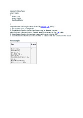
We further illustrate the importance of the asymptotic viewpoint in Table 3.3.
This table explores the maximum size allowed for an input instance that is pro-
cessed by an algorithm in 1 second, 1 minute, and 1 hour. It shows the importance
of good algorithm design, because an asymptotically slow algorithm is beaten in
the long run by an asymptotically faster algorithm, even if the constant factor for
the asymptotically faster algorithm is worse. Running
Maximum Problem Size (n) Time (µs) 1 second 1 minute 1 hour 400n 2,500 150,000 9,000,000 2n2 707 5,477 42,426 2n 19 25 31
Table 3.3: Maximum size of a problem that can be solved in 1 second, 1 minute,
and 1 hour, for various running times measured in microseconds.
Tài liệu liên quan:
-
Bài mẫu cấu trúc dữ liệu và giải thuật Môn Câu trúc dữ liệu giải thuật | Trường Đại học Công nghiệp Thành phố Hồ Chí Minh
124 62 -
Bài tập thực hành CTDL - Tóm tắt Cấu trúc Dữ liệu & Giải thuật Môn Câu trúc dữ liệu giải thuật | Trường Đại học Công nghiệp Thành phố Hồ Chí Minh
108 54 -
Thực hành Môn Câu trúc dữ liệu giải thuật | Trường Đại học Công nghiệp Thành phố Hồ Chí Minh
124 62 -
Bài tập thực hành Môn Câu trúc dữ liệu giải thuật | Trường Đại học Công nghiệp Thành phố Hồ Chí Minh
129 65