


Preview text:
1 Bài 2.9 a. yi = β1 + β2xi + ei and E[ei | x1] = 0 y1 + y2 + y3 1 ¯ y 1 = =
(β1 + β2x1 + e1) + (β1 + β2x2 + e2) + (β1 + β2x3 + e3) 3 3 ⇒ ¯ y1 = β1 + β2 ¯ x1 + ¯ e1 x1 + x2 + x3 e1 + e2 + e3 ¯ x1 = , ¯ e1 = 3 3 y4 + y5 + y6 ¯ y2 = 3 ⇒ ¯ y2 = β1 + β2 ¯ x2 + ¯ e2 x4 + x5 + x6 e4 + e5 + e6 ¯ x2 = , ¯ e2 = 3 3 ¯ y2 − ¯ y1 (β1 + β2 ¯ x2 + ¯ e2) − (β1 + β2 ¯ x1 + ¯ e1) ¯ e2 − ¯ e1 we have ˆ β2,mean = = = β2 + ¯ x2 − ¯ x1 ¯ x2 − ¯ x1 ¯ x2 − ¯ x1 E[¯ e2 − ¯ e1 | x] E[ ˆ
β2,mean | x1, x2, .., x6] = β2 + (since E[ei | x] = 0) ¯ x2 − ¯ x1 E[¯ e1 | x] = 0, E[¯ e2 | x] = 0 ⇒ E[¯ e2 − ¯ e1 | x] = 0 E[ ˆ β2 | x,.., x6] = β2
b. Assuming assumptions SR1–SR6 hold, show that E( ˆ β2,mean) = β2. Solution.
Using the law of iterated expectations, h i E( ˆ β2,mean) = E E( ˆ β2,mean | x) . From part (a), E( ˆ β2,mean | x) = β2. Therefore, E( ˆ β2,mean) = β2. c. We have ˆ ¯ e2 − ¯ e1 β2,mean = β2 + , ¯ x2 − ¯ x1 where 3 6 1 X 1 X ¯ e1 = ei, ¯ e2 = ei. 3 3 i=1 i=4
Since β2 is a constant, the cohavditional variance given x is ¯ e 2 − ¯ e1 Var( ˆ β 2,mean | x) = Var x . ¯ x 2 − ¯ x1 1 Var( ˆ β2,mean | x) = Var(¯ e2 − ¯ e1 | x). (¯ x2 − ¯ x1)2
Under assumptions SR1–SR6, the error terms are independent and satisfy Var(ei | x) = σ2. Therefore, σ2 σ2 Var(¯ e1 | x) = , Var(¯ e2 | x) = . 3 3 2
Because the two groups of errors are independent, we obtain 2σ2 Var(¯ e2 − ¯ e1 | x) = . 3 Hence, 2σ2 Var( ˆ
β2,mean | x) = 3(¯x2 − ¯x1)2
For comparison, the conditional variance of the ordinary least squares estimator is σ2 Var(b2 | x) = . P6 (x i=1 i − ¯ x)2
Professor Mean’s estimator uses only two sample means instead of all six observations. As a result, it exploits less
information than the OLS estimator and is therefore less efficient. Consequently, Var( ˆ
β2,mean | x) > Var(b2 | x). Bài 2.24 1 2 setwd("D:/KTL") 3 data=read.csv("ashcan.csv") 4 data 5
data_sold=subset(data, sold == 1) 6 data_sold 7
mean_rh =mean(data_sold$rhammer, na.rm = TRUE) 8
median_rh =median(data_sold$rhammer, na.rm = TRUE) 9
quantiles_rh =quantile(data_sold$rhammer, probs = c(0.25, 0.75), na.rm = TRUE) 10 11 summary(data_sold$rhammer) 12 13 a. 1 # Vẽ Histogram cho RHAMMER 2
hist(data_sold$rhammer, breaks = 30, main = "Histogram of RHAMMER", 3
xlab = "Price (RHAMMER)", col = "lightblue", border = "black") 4 3 b. 1
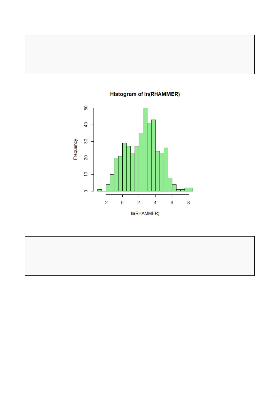
# Tạo bién log của RHAMMER 2
data_sold$ln_rhammer = log(data_sold$rhammer) 3 4
# Vẽ Histogram cho ln(RHAMMER) 5
hist(data_sold$ln_rhammer, breaks = 30, main = "Histogram of ln(RHAMMER)", 6
xlab = "ln(RHAMMER)", col = "lightgreen", border = "black") 7 c. 1
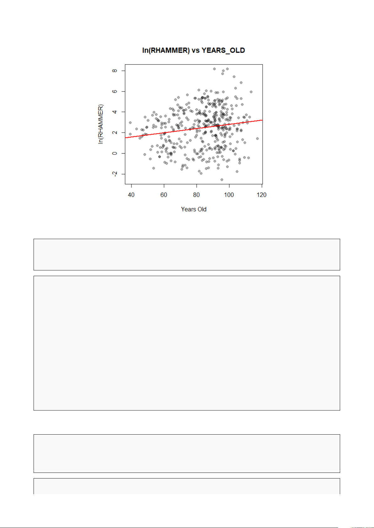
# Vẽ đò thị phân tán và đưòng hòi quy 2
plot(data_sold$years_old, data_sold$ln_rhammer, 3
main = "ln(RHAMMER) vs YEARS_OLD", 4
xlab = "Years Old", ylab = "ln(RHAMMER)", pch = 19, col = rgb(0,0,0,0.3)) 5
model_c=lm(ln_rhammer ~ years_old, data = data_sold) 6
abline(model_c, col = "red", lwd = 2) 7 4 d. 1 # Hòi quy theo YEARS_OLD 2
model_d = lm(ln_rhammer ~ years_old, data = data_sold) 3 summary(model_d) 4 1 Call: 2
lm(formula = ln_rhammer ~ years_old, data = data_sold) 3 4 Residuals: 5 Min 1Q Median 3Q Max 6 -5.253 -1.535 0.133 1.450 5.561 7 8 Coefficients: 9
Estimate Std. Error t value Pr(>|t|) 10 (Intercept) 0.75792 0.50541 1.500 0.134463 11 years_old 0.02043 0.00597 3.422 0.000683 *** 12 --- 13 Signif. codes:
0 ’***’ 0.001 ’**’ 0.01 ’*’ 0.05 ’.’ 0.1 ’ ’ 1 14 15
Residual standard error: 1.972 on 420 degrees of freedom 16 Multiple R-squared: 0.02712, Adjusted R-squared: 0.02481 17
F-statistic: 11.71 on 1 and 420 DF, p-value: 0.0006827 18 19 Hình 1: Kết quả code e. 1
# Hòi quy theo DREC (bién giả suy thoái) 2
model_e = lm(ln_rhammer ~ drec, data = data_sold) 3 summary(model_e) 4 5 1 Call: 2
lm(formula = ln_rhammer ~ drec, data = data_sold) 5 3 4 Residuals: 5 Min 1Q Median 3Q Max 6 -5.0976 -1.6304 0.1207 1.3549 5.6229 7 8 Coefficients: 9
Estimate Std. Error t value Pr(>|t|) 10 (Intercept) 2.5547 0.1011 25.267 < 2e-16 *** 11 drec -1.0420 0.3284 -3.173 0.00162 ** 12 --- 13 Signif. codes:
0 ’***’ 0.001 ’**’ 0.01 ’*’ 0.05 ’.’ 0.1 ’ ’ 1 14 15 16
Residual standard error: 1.976 on 420 degrees of freedom 17 Multiple R-squared: 0.02341, Adjusted R-squared: 0.02108 18
F-statistic: 10.07 on 1 and 420 DF, p-value: 0.00162 19 20 Hình 2: Kết quả code