A novel hybrid model based on neural network and multi-objectiveoptimization for effective load forecast | Tiếng Anh 12
A novel hybrid model based on neural network and multi-objectiveoptimization for effective load forecast | Tiếng Anh 12
Chủ đề: Tài liệu chung Tiếng Anh 12 528 tài liệu
Môn: Tiếng Anh 12 1.3 K tài liệu
Tác giả:


Preview text:
Energy 182 (2019) 606e622
Contents lists available at ScienceDirect Energy
j o u r n a l h o me p a g e : w w w . e l s e v i e r . c o m/ l o ca t e / e n e r g y
A novel hybrid model based on neural network and multi-objective
optimization for effective load forecast
Priyanka Singh*, Pragya Dwivedi
Computer Science and Engineering Department, MNNIT Allahabad, Allahabad, 211004, India a r t i c l e i n f o a b s t r a c t Article history:
In recent years, increased attention has been paid by the researchers to predict accurate and stable load Received 17 January 2019
due to its effect on the economy and need for proper management of power systems. However, most of Received in revised form
the previous research focused only on either reducing load forecast error or enhancing the stability, very 21 May 2019
few studies focused on these two issues simultaneously. Introducing a forecasting model to solve both Accepted 10 June 2019
independent objectives at the same time is a challenging task due to the complex behavior of the load Available online 14 June 2019 pattern.
Therefore, to achieve two objectives simultaneously, we propose a novel multi-objective algorithm Keywords:
(MOFTL) based on Follow The Leader algorithm. The effectiveness of MOFTL has been shown by Load forecasting Artificial neural network
comparing the results with three newly presented MOWCA, MOPSO and NSGA-II multi-objective algo- Multi-objective optimization
rithms. Moreover, to validate the performance of MOFTL, we have combined MOFTL with neural network Hybrid forecasting model
termed as MOFTL-ANN to solve the problem of electricity load forecasting. The proposed hybrid model
Multi-objective follow the leader (MOFTL)
outperforms baseline models over two real-world electricity data sets namely England region and ERCOT
region. MOFTL-ANN shows improvement of 17.42%, 6.81%, 10.77% and 59.69% MAPE values for England
region and 4.20%, 4.16%, 1.14% and 21.85% MAPE values for ERCOT region over NSGA-II-ANN, FTL-ANN, BPNN, and GRNN.
© 2019 Elsevier Ltd. All rights reserved. 1. Introduction
development of an effective model with enhanced forecasting
abilities for accurate and stable load estimation is desired. So far,
Load forecasting is a central and integral process for periodic
several techniques and models have been proposed for load fore-
planning, scheduling, controlling load generation, continuous dis-
casting. In the initial stages of load forecasting, classical statistical
tribution of electricity and expansion of facilities in the power
techniques like BoxeJenkins models and time series techniques
sectors [1,2]. Meanwhile, the study of load forecasting is a chal-
were widely used in load forecasting [6,7]. However, load data have
lenging task due to several uncertain factors such as demand
complex behavior [8] and are influenced by several factors [9], time
fluctuation, complex historical load curve, calendar effects, fore-
series techniques may exhibit poor performance. Thus, several
casting models, random effects and many more [3].
artificial intelligence techniques including artificial neural net-
In the past few years, load forecasting has been a very active and
works (ANNs) [10e13], fuzzy logic [14e16], expert systems, and
popular research topic because of several reasons, deregulation of
support vector machines (SVMs) [17,18] have been applied to time
the electricity market, increased fluctuation in energy demands
series forecasting. Among these techniques, ANN has been widely
and increased operating costs [4]. The poor forecasting methods
used for solving load forecasting problem [19e21].
result in considerable losses to the economy, for example, a
Apart from these techniques, several hybrid models have been
research in 1985 presented that 1% increase in forecasting error
presented in the literature to yield forecasting results with extreme
increased the associated operating costs of up to 10 million pounds
accuracy [33]. To find optimal hybrid model, several optimization
every year in the thermal British power system [5]. Therefore, the
algorithms, such as particle swarm optimization (PSO) [34], genetic
algorithm (GA) [35], artificial bee colony (ABC) [36], differential
evolutionary (DE) [37,38], cuckoo search (CS) algorithm [39,40], ant * Corresponding author.
colony algorithm [41] and follow the leader (FTL) [30] algorithm E-mail addresses: 2015rcs53@mnnit.ac.in, priyankamnnit925@gmail.com
have been applied for load prediction. In these studies [7,30,34,35],
(P. Singh), pragyadwi86@mnnit.ac.in (P. Dwivedi).
https://doi.org/10.1016/j.energy.2019.06.075
0360-5442/© 2019 Elsevier Ltd. All rights reserved.
P. Singh, P. Dwivedi / Energy 182 (2019) 606e622 607
researchers focused on improving the accuracy of forecasting
a MOP is to find the set of solution termed as a Pareto-optimal set
models by finding optimal weights of ANN, but stability also plays a
which lies on the Pareto Front (PF) and, solutions have uniform
vital role in determining the effectiveness of a forecasting model.
distribution along the true PF [44,51]. Among multiple trade-offs
Considering only one objective (accuracy or stability) at a time is
and solutions found, choose only one solution using higher-level
insufficient for finding effective load forecasting model. Thus, a
information for practical purpose [46]. From the fact that multi-
hybrid model based on ANN should optimize the initial weights
objective algorithms can approximately find the true Pareto-
while considering accuracy and overcome the instability of the final
optimal solutions of most MOPs, we have proposed a novel results simultaneously.
multi-objective algorithm called Multi-Objective Follow The Leader
Researchers have developed an indefinite number of learning
(MOFTL). This algorithm overcomes the problem of solving a single
algorithm that are accurate and predicts outcomes with a high
objective function and enhance the accuracy and stability simul-
degree of confidence. But what happens when training the model taneously for load prediction.
with a different/same subset of same training data set, will the
To obtain higher accuracy and better stability for load prediction
model perform with the same efficiency over repeated experi-
at the same time, a novel hybrid model involving the widely
ments. ANN depends on random initial values, therefore, the final
acceptable neural network (NN), and our proposed multi-objective
outcome varies over the same input data set. Every predictive
algorithm (MOFTL) is presented in this paper. The validation of our
model has to be accurate and stable. A learning model is stable
proposed multi-objective algorithm is done by testing on four
when the predicted result does not change more than a certain
multi-objective benchmark problems and comparing with three
threshold for the different/same subset of data set over several
newly developed multi-objective algorithms: MOWCA, MOPSO,
experiments. It is noteworthy that a hybrid model that achieves
and NSGA-II. For a comprehensive evaluation of MOFTL, hybrid
high accuracy and strong stability at the same time is a multi-
forecasting model MOFTL-ANN has been presented and applied for
objective problem (MOP) rather than a single-objective problem.
load forecasting over two electricity load data sets collected from
Over the past few decades, multi-objective problems (MOPs)
England and Texas. Results obtained from different forecasting
have attracted researchers in different real-world problems [42,43].
models are tested by the Friedman test to show their statistical
Many multi-objective algorithms such as binary coded elitist non- significance.
dominated sorting GA (NSGA-II) [44e46], multi-objective ant lion
The major contributions of our work are as follows:
optimizer (MOALO) [47,48], multi-objective flower pollination al-
gorithm (MOFPA) [49], multi-objective firefly algorithm (MOFA) [1],
A novel multi-objective follow the leader, MOFTL algorithm is
multi-objective whale optimization algorithm (MOWOA) [50] etc. proposed in this paper.
have been introduced in last few years. Table 1 shows the research
To validate the effectiveness of MOFTL, it is tested on four multi-
contribution of different forecasting models. Findings from this
objective benchmark problems and compared with three multi-
literature prove that hybrid forecasting models generate less fore-
objective algorithms: MOWCA, MOPSO, and NSGA-II.
casting error. But stability of the model is another important factor
Further to obtain higher accuracy and excellent stability for load
in load forecasting that cannot be ignored. Based on the findings,
forecasting, we combined MOFTL with a neural network called
we can conclude that multi-objective optimization algorithms
MOFTL-ANN to optimize network weights.
overcome the shortcomings of single-objective optimization algo-
The comprehensive evaluation of MOFTL-ANN shows that it
rithms and achieve improvement in accuracy and stability simul-
overcomes the problem of solving single objective functions and
taneously. MOPs generate a series of optimal solutions, named
enhance the accuracy and stability for load forecasting.
Pareto-optimal solutions (solutions are equally optimal) for solv-
ing different conflicting objectives simultaneously. The ideal goal of
The paper is organized as follows. Section 2 briefly describes Table 1
Research contributions of forecasting algorithms in electricity load forecasting. S.no. Forecasting Methodology Findings algorithm 1 Linear
In Ref. [22], a regression-based daily peak load forecasting method with a Linear regression fails for nonlinear data due to poor non-linear fitting regression
transformation technique is proposed. capability, lacks accuracy. 2 Multi
In Ref. [23], for mid-term load forecast on an hourly basis of US utility,
Multi regression technique has received limited success, it generates regression
multi-regression model has been used.
higher forecasting error for abrupt changes in the environment. 3
Exponential In Ref. [24], five developed exponential smoothing models are compared They are faster and efficient but generates more error for a long-term load smoothing
over one day ahead load forecast. forecast. 4 ARIMA
In Ref. [25], ARIMA model and transfer function model are applied to STLF ARIMA model generates great results for linear problems but is incapable
by considering weather and load relationship.
of solving nonlinear sensitive part of the load, it generates results only on
the basis of past and current data. 5 Fuzzy logic
In Ref. [26], a fuzzy logic method is employed to forecast the gross
Fuzzy techniques generate better forecast results than statistical models. It electricity demand of Turkey.
provides reliable result but shows a strong dependency on expert systems. 6 SVR
In Ref. [9], a generic STLF strategy based on the support vector regression SVR is a robust and accurate method. It is a highly effective model in
machines is proposed. In Ref. [27], SVR is used to find demand response for solving non-linear problems but fails due to higher running time and high an office building.
dependency between forecasting accuracy and selected SVM parameters. 7 ANN
In Ref. [28], multilayer perceptron model (MLP) is used for the prediction of ANN has the capability to map the complex input and output relationship
long-term energy consumption. In Ref. [29], LSTM recurrent neural
but due to restricted generalization ability, the solution falls in a local
network is used to solve the problem of load forecasting in a residential
minimum. Also, for large neural network, high running time is required. area. 8 Hybrid
In Ref. [30], a newly proposed evolutionary algorithm is combined with
The efficiency of the hybrid model is improved in terms of accuracy but models
ANN to enhance forecasting accuracy. In Ref. [31], GRNN is combined with stability of model is another important factor that needs to be considered
a fruit fly optimization algorithm to improve the capability of GRNN for during the load forecast.
power load forecasting. In Ref. [32], modified firefly algorithm is used to
find the optimal parameters of support vector regression. 608
P. Singh, P. Dwivedi / Energy 182 (2019) 606e622
multi-objective optimization and proposed multi-objective algo-
population [52]. In other words, crowding distance is a measure of
rithm. Section 3 presents the proposed hybrid model and section 4
how close an individual is to its neighboring candidates within
demonstrates the performance of MOFTL over four multi-objective
population [1]. It is always desired that location of solutions in
benchmark problems and numerical results obtained from the
same front level have uniform distribution as, a large diversity of
proposed hybrid model for electricity load forecast problem. In
the individuals can solve the stagnation problem of multi-objective
Section 5, discussions based on experimental results are intro-
algorithms. Firstly, individuals are sorted on the basis of every mth
duced. Section 6 presents the conclusions of this paper.
objective function then boundary individuals of each level are
assigned infinite value and crowding distance of other individuals
2. Multi-objective follow the leader algorithm are calculated as follows.
In this section, the concept of multi-objective optimization and D1 ¼ ∞
some related description of the MOFTL are described. Dn ¼ ∞ (2) Xn1XM f m
2.1. Multi-objective optimization D iþ1 f m i1 i ¼ i¼2 m¼1f max m f min m
Solving one objective function by an evolutionary algorithm is
single-objective optimization problem where an optimal solution is
where D1 and Dn are boundary individuals at each PF, n is number
chosen very conventionally. However, multi-objective optimization of individuals at each PF, f m
i is fitness value of mth objective function
problem solves more than one problem simultaneously. Unlike
of ith individual at PF f and m is number of objective functions and
single-objective optimization problem the output of MOP is series the parameters f max m and f min m are the maximum and minimum
of solutions called Pareto-optimal solutions, which are equally
values of the mth objective function. Larger the average crowding
optimal and their mapping in objective space generates Pareto
distance, better is the diversity in the population.
Front [47]. Selection of Pareto-optimal solutions that are uniformly
distributed along true Pareto Front is recommended. The definition
2.2. MOFTL (multi-objective follow the leader)
of multi-objective optimization problem, Pareto dominance, crowding distance are given as follows.
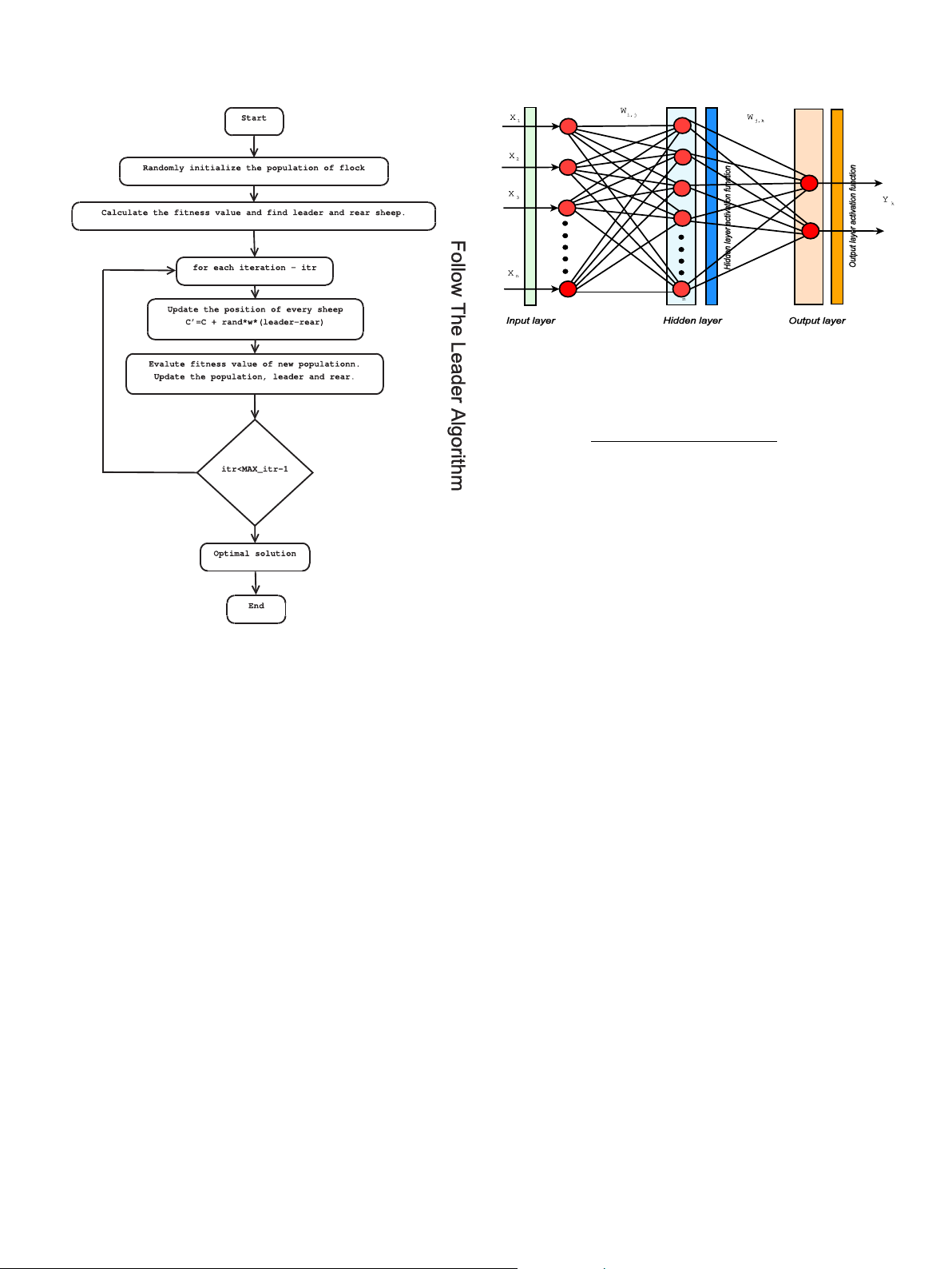
MOFTL is a multi-objective version of a novel meta-heuristic FTL
Definition 1. Multi-objective optimization problem [52].
algorithm proposed by Singh and Dwivedi in 2018 inspired from 8 9
moving behavior of a sheep [30,54]. In flock, sheep having highest > >
score is leader candidate and one with the lowest score is rear > > > Minimize=Maximize : f mðxÞ; m ¼ 1; 2; …::; M; > < > > Subject to : g =
candidate. When leader moves within the flock, other candidates jðxÞ 0; j ¼ 1; 2; …::; J; >
follow them. Mathematical representation for updating the posi- > h > kðxÞ ¼ 0; k ¼ 1; 2; …::; K; > > > : >
tion of every candidate is shown in eq. (2). xðLÞ x ; i ¼ 1; 2; …::; n; > ; i i xðUÞ i 0 (1) X ¼ X X (3) j;k;i j;k;i þ randu* j;leader;i Xj;rear;i
where M, J, K, n represents number of objective functions,
where, X0j;k;i is updated position of sheep Xj;k;i, Xj;leader;i is position
inequality constraints, equality constraints and number of vari-
value of the variable j for leader sheep in ith iteration, Xj;rear;i is
ables, respectively. xðLÞ and xðUÞ are lower and upper boundaries of i i
position value of the variable j for rear sheep in ith iteration, rand is xi for ith variable.
a random value between 0 and 1 and u is inertia weight value lying
between 0 and 1 to control exploration and exploitation process
Definition 2. Pareto Dominance: [52] A solution xð1Þ is said to
within the solution space. Fig. 1 shows sequential flowchart of FTL.
dominate the other solution xð2Þ, if both the following conditions
Unlike single-objective FTL, multi-objective FTL has several are true:
objective functions and should be evaluated simultaneously. A set
of non-dominated solutions are generated by checking domination
The solution xð1Þ is no worse than xð2Þ in all objectives. Thus, the
condition between two solutions. In MOFTL, all the solutions are
solutions are compared based on their objective function values
distributed within different front levels based on dominance con-
(or location of the corresponding points (zð1Þ and zð2Þ) on the
dition. Top front level ranks first in which no individual is domi- objective space).
nated by other individuals, individuals in the second level are
The solution xð1Þ is strictly better than xð2Þ in at least one
dominated by some individuals on level 1, and so on. In the same objective.
front level, there exist a number of solutions that are distributed
which is expected to be in a uniform manner, the crowding distance
Based on comparison of dominance value, all individuals are
operator helps in the selection process and measures closeness
sorted into different front levels. Each front level has a rank, which
between an individual and its neighbors. Larger average crowding
equals its non domination level. The individual in level 1 are
distance brings greater diversity in the population. For solving load
dominated by no other individuals; the individual in level 2 is
forecasting problem with MOFTL, we have considered two objec-
dominated by individuals of only level 1, and so on.
tive functions mean squared error (MSE) and standard deviation
Definition 3. Crowding Distance: [44]
(STD) to represent accuracy and stability respectively. The equation
For MOPs, there is more than one objective function to be
of objective functions for load forecasting can be defined as follows:
minimized or maximized. To select the best solution in the popu-
lation that satisfies the condition of all objective function simul- 1 X n MSE ¼ ðy0
taneously, crowding-distance mechanism is used [53]. The N i yiÞ2 (4) i¼1
crowding distance of an individual is a measure of objective space
of individual that is not occupied by any other solution in the
P. Singh, P. Dwivedi / Energy 182 (2019) 606e622 609
Fig. 2. Feed forward neural network. [30]: 0 1 X m 1 Y @ A k ¼ Wk;j: P þ Q n j (6) j¼1 1 þ exp i¼1Wj;iXi þ Qj
where, 1in, 1 j m Wi;j represents weight between nodes i
and j, Qj is activation function of jth node and n and m represents
number of nodes in input and hidden layer respectively.
So far several optimization algorithms have been combined
with neural network to find optimal weights such as genetic al-
gorithm [35], PSO [60], fruit fly optimization algorithm [31] to
predict accurate load forecasting. But finding a model that precisely
generate load along with greater stability is bigger problem of load
forecasting. Thus, a novel multi-objective algorithm has been pro-
Fig. 1. Flowchart of FTL algorithm.
posed in this paper which can not only predicts load with high
precision but also stable forecasting.
STD ¼ stdðy0i yiÞ; i ¼ 1; 2; …:N (5)
3.2. The MOFTL-ANN hybrid model
In this section, the weights of neural network are updated by a
3. Proposed hybrid forecasting model
multi-objective optimization algorithm, MOFTL to allow ANN to
achieve enhanced accuracy and stability simultaneously. For
In this section, detailed study of artificial neural network and
effective load forecasting, it is recommended to consider both ac-
hybrid MOFTL-ANN model is introduced.
curacy and stability at the same time. Thus, the optimization of
initial weights of a neural network should satisfy both the objective
3.1. Artificial neural network
functions simultaneously. Mean squared error (MSE) f1 in fore-
casting are highly considered for performance evaluation of load
An artificial neural network (ANN) is intelligence-based learning
forecasting models. In this study, standard deviation of forecasting
system, inspired from functioning of human brain which consists of
error is chosen as another indicator for representing the stability of
several small processing elements called neurons [55,56]. These
a forecasting model f2. Smaller the mean squared error and stan-
neurons are interconnected and these connection have some
dard deviation value, higher is the accuracy and stability. The
weight associated with themselves. Neurons receive information
pseudo-code of the hybrid MOFTL-ANN model is presented in Al-
through several input nodes, process them internally and generates gorithm 1.
a response [57]. ANN being universal approximator can approxi-
mate large class of functions, generate higher accuracy over other
nonlinear model [58]. ANN architecture is composed of three 4. Experiments and analysis
layers: input layer, hidden layer and output layer. In input layer,
significant features which shows impact on prediction are consid-
To verify the effectiveness of the proposed multi-objective al-
ered and hidden layer/layers use these features to generate inter-
gorithm and hybrid model, two different experiments are per-
mediate solution and final predicted value is produced at output
formed. In experiment 1, MOFTL is compared with three newly
node of network [59]. Usually, feed forward neural network with
developed multi-objective algorithms namely MOWCA [53,61],
single hidden layer is preferred in time series forecasting. A simple
MOPSO [62], and NSGA-II [46]. In Experiment II, the performance of
architecture of feed forward neural network is shown in Fig. 2.
hybrid model (MOFTL-ANN)is compared with five state-of-art
Mathematical representation of relationship between inputs X ¼
forecasting models. Here, the obtained results are compared over
X1; X2; …::Xn and output Yk for logistic activation function in hidden
two load data sets namely, England region and ERCOT region. De-
layer and linear function in output layer can be shown as follows
tails of the experiment are described in the following subsections. 610
P. Singh, P. Dwivedi / Energy 182 (2019) 606e622
4.1. Experiment I: tests of MOFTL
forecasting problem. Implementation details are discussed in the forthcoming subsections.
In this experiment, four multi-objective problem and three well
known multi-objective algorithms namely MOPSO, MOWCA and 4.3. Data pre-processing
NSGA-II have been used to test and compare the performance of
MOFTL algorithm. Mathematical representation of multi-objective
Before going for load prediction, data pre-processing is done to problems are as follows:
eliminate spikes and outliers. The missing and extra data values are
managed and data normalization (MIN-MAX) is done between the
interval of ½ 1; 1 to reduce the training time. To perform different FON:
experiments, the data set is divided into training and testing data. ! P 1 2 Minimize : f ð1Þ ¼ 1 exp 3 pffiffiffi i¼1 xi 3 4.4. Evaluation metrics ! P 1 2 Minimize : f ð2Þ ¼ 1 exp 3 pffiffiffi i¼1 xi þ 3
Since the past few decades, several evaluation metrics have where; 4 xðiÞ 4
been developed to evaluate the performance of the load forecast. SCH:
However, there are no predefined rules for selecting these metrics. Minimize : f ð1Þ ¼ x2
In this paper, we use the nine commonly used evaluation metrics Minimize : f ð2Þ ¼ ðx 2Þ2
shown in Table 3 to evaluate the performance forecasting models. where; 103 xðiÞ 103
Mean absolute error (MAE) indicate the overall level of errors [50]. ZDT1:
Normalized mean squared error (NMSE) calculates the overall de- Minimize : f ð1Þ ¼ xð1Þ sffiffiffiffiffiffiffiffiffi !
viations between forecasted and measured load. The root of mean xð1Þ Minimize : f ð2Þ ¼ g* 1 squared error (RMSE) re g
flects the degree of differences between the X
predicted and measured values and is more stable than MSE and 9 N where : g ¼ 1 þ xðiÞ and 0 xðiÞ 1; 1 i n n 1 i¼2
less sensitive to extreme errors. Mean absolute percent error ZDT3:
(MAPE) shows accuracy as a percentage of forecasting error. Minimize : f ð1Þ ¼ xð1Þ ffiffiffiffiffiffiffiffi s ffi
Directional Change (DC) exhibits the movement directions or ! xð1Þ xð1Þ
turning points of prediction. Pearson's correlation coef Minimize : f ð2Þ ¼ g* 1 sinð10pxð1ÞÞ ficient (r) g g
shows the correlation between the predicted value and the 9 XN where : g ¼ 1 þ xðiÞ and 0 xðiÞ 1; 1 i n
observed value. Lastly, the index of agreement (IA) is a standard n 1 i¼2
metric of the degree of model prediction error [64]. In the following
subsections, we present two case studies on various data sets to
These four test functions and the performance metrics of
validate the effectiveness of MOFTL-ANN. ALL the experimental
reverse generational distance (RGD) [63] along with three newly
parameters involved during the experiment is shown in Table 5.
developed multi-objective algorithms- MOWCA, MOPSO, and
The experiment has been performed 100 times with population
NSGA-II verify the performance of our proposed algorithm MOFTL.
size of 50, 5,000 maximum iteration, 10 hidden neurons, one
The mathematical formula for RGD is shown in eq. (7).
output neuron and the number of input neurons is same as the
ffiffiffiffiffiffiffiffiffiffiffiffi v ffi
number of input parameters taken in the case study. u
In order to validate the performance of our proposed hybrid 1 X N u RGD ¼ t d2 (7)
model MOFTL-ANN, we have compared our model to following N j j¼1 state-of-art models.
where, dj is Euclidean distance between ith true PF and nearest
NSGA-II-ANN (Neural network with NSGA-II)
members of obtained PF and N is number of true PF.
FTL-ANN (Neural network with Follow the leader algorithm)
Each test function has been performed 100 times for 500 iter-
BPNN (Backpropagation neural network)
ations and 100 population to find Pareto optimal solutions. The
GRNN (Generalized regression neural network)
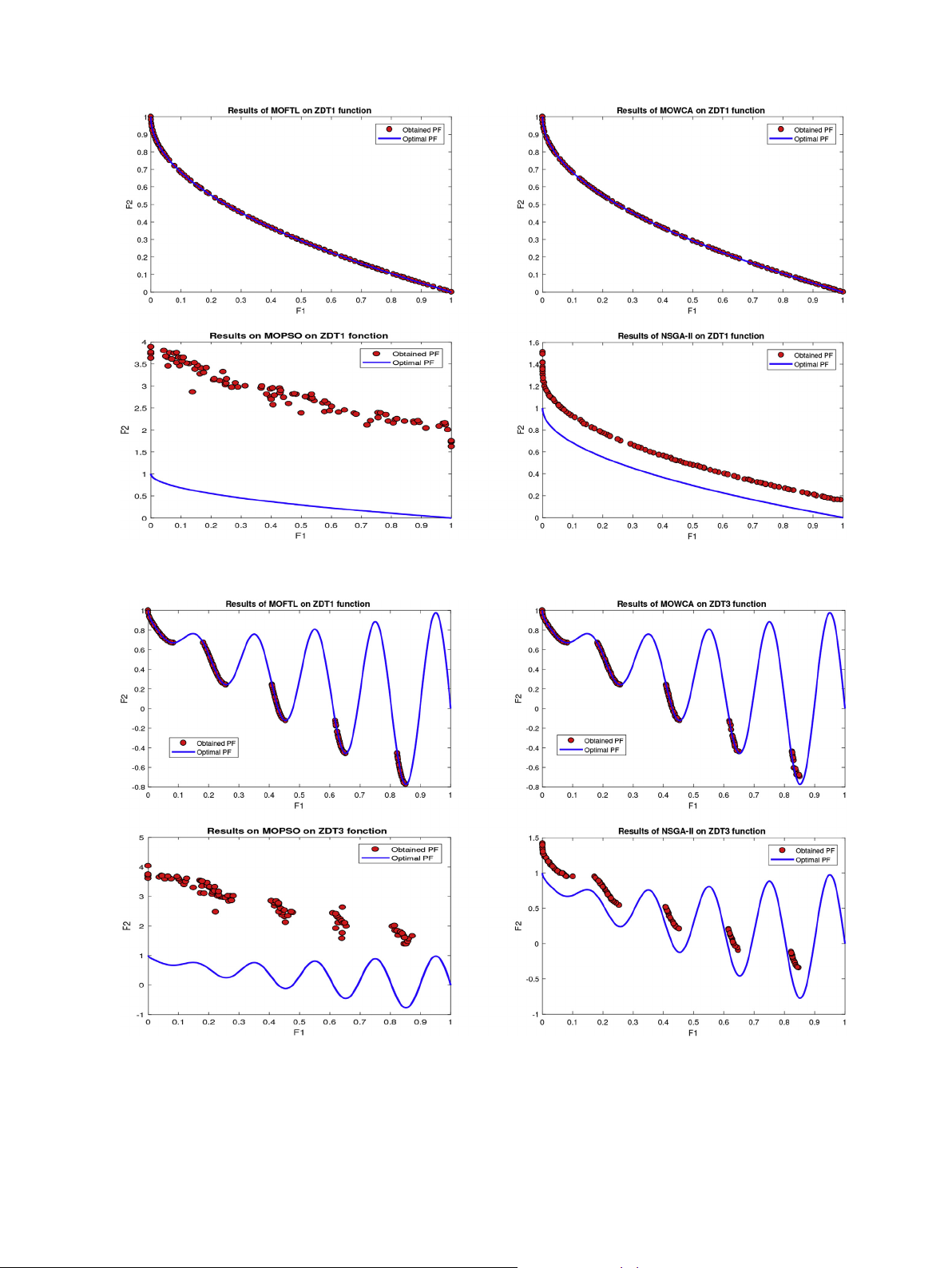
results obtained from the experiment are shown in Table 2 and
Figs. 3e6. From Table 2, it can be easily demonstrated from all the
statistical values that MOFTL is superior to MOWCA, MOPSO, and 4.5. Case study-1: ISO England
NSGA-II. Our proposed multi-objective algorithm yields the best
values of standard deviation for FON- 0.000156, SCH- 0.000366, 4.5.1. Data description
ZDT1- 0.010104 and ZDT3- 0.002242 multi-objective problems.
Hourly data set from England region from years 2004e2007 and
And these results prove that lower is standard deviation lesser in
out-of-sample data from the years 2008 and 2009 are used for
scattering and better is the solution.
training and testing purpose [65]. The statistical parameter of data
Remark. Results shown proves that MOFTL performs well and is
set is shown in Table 4 and the correlation coefficient (r) between
superior to MOWCA, MOPSO, NSGA-II. MOFTL achieves better
independent variables given as input to a neural network and load
optimal solutions than others with higher accuracy and also finds
is shown in Table 6. Higher the value of r higher is the correlation
the best values of RGD. Thus, results show that our proposed al-
between the input parameter and load.
gorithm is effective and can be further used for solving real-world
multi-objective problems such as load forecasting problem of 4.5.2. Result
predicting load with higher accuracy and stability.
The results obtained for the year 2008 and 2009 by all the
forecasting models are shown in Table 7 with their minimum,
4.2. Experiment II: tests of MOFTL-ANN
average and maximum values. It clearly shows that MOFTL-ANN
brings higher accuracy in terms of all performance evaluation
To deeply analyze the superior performance of the proposed
metrics mentioned earlier. Moreover, from the table, it can be
algorithm, MOFTL is implemented to solve the short-term load
observed that MOFTL enhances the prediction ability of ANN than
P. Singh, P. Dwivedi / Energy 182 (2019) 606e622 611 Table 2
Results of the multi-objective algorithms (using RGD) on the four test functions adopted in this paper. Algorithm FON Algorithm SCH Min Avg Median Max Std. Min Avg Median Max Std. MOFTL 0.00447282 0.00478 0.004756 0.005365 0.000156 MOFTL 0.01701711 0.017963 0.01793 0.018785 0.000366 MOWCA 0.01363076 0.117798 0.096826 0.429674 0.093677 MOWCA 0.01883266 0.020035 0.020002 0.021894 0.000675 MOPSO 0.0045397 0.00491 0.004892 0.005431 0.00019 MOPSO 0.01927343 0.021082 0.02084 0.026767 0.001125 NSGA-II 0.00437934 0.004857 0.004838 0.005422 0.000204 NSGA-II 0.01937874 0.021189 0.021199 0.023965 0.000993 Algorithm ZDT1 Algorithm ZDT3 Min Avg Median Max Std. Min Avg Median Max Std. MOFTL 0.004333 0.008895 0.004785 0.340285 0.010104 MOFTL 0.190448 0.192423 0.191566 0.208109 0.002242 MOWCA 0.004412 0.026285 0.004876 0.319874 0.057746 MOWCA 0.191381 0.195551 0.19257 0.303958 0.01236 MOPSO 1.143838 1.457361 1.459175 1.615171 0.077166 MOPSO 0.804463 1.081175 1.092714 1.276132 0.09646 NSGA-II 0.111613 0.137112 0.13742 0.173442 0.033702 NSGA-II 0.195631 0.20023 0.199969 0.237757 0.00471 Algorithm 1: MOFTL-ANN. Objective Functions: 8 9 < = f Minimize 1 ðxÞ ¼ MSE : f2ðxÞ ¼ STD ; Input: Xtrain - training samples Xtest - testing samples Output: Xforecast - forecasting data Parameters:
Maxit - maximum number of iterations
Npop - number of sheep within a flock Dim - number of dimensions Xi - position of ith sheep Ri - rank value of ith sheep
di - crowding distance values of ith sheep
Fi - fitness values of ith sheep Begin
1 Set all the input parameters of MOFTL.
2 Initialize random positions of all sheep within the flock of size Npop and Dim dimensions in the range of - 1 and þ 1.
3 For each sheep i within the flock i ¼ 1:Npop
4 Compute corresponding fitness function f1 and f2 using non-dominated sort ranking process.
5 Calculate crowding distance di. 6 end for 7
=* Determine leader Xleader and rear Xrear sheep on the basis of their rank and crowding distance. = 8 While (i < Maxit) 9
=* Evaluate new solution and update position of sheep =
10 For each sheep i within the flockj¼1:Npop 11 For k¼1:Dim 0 12 X ¼ X j;k;i
j;k;i þ randu*ðXj;leader;i Xj;rear;iÞ 13 end for 14 end for 15
=* Check if any sheep goes beyond the boundary conditions. =
16 For each sheep i within the flock i ¼ 1:Npop
17 Compute corresponding fitness function f1 and f2 using non-dominated sort ranking process.
18 Calculate crowding distance di. 19 end for
20 = Selection of sheep for next generation. =
21 Merge X0 and X, sort them on the basis of rank and
crowding distance and update X with Npop sheep.
22 = Update leader and rear sheep. = 23 end while 24 Return X
25 Set the weights of neural network according to X. 26 Use Xtrain to train ANN.
27 Use electricity load test data set Xtest to obtain the predicted valve Xforecast. End
NSGA-II does. For example, minimum values for MAPE of MOFTL-
forecasting model. However, MOFTL-ANN generates higher accu-
ANN and NSGA-II-ANN are 3.2019% and 3.9615%, respectively. The
racy than FTL-ANN as the reason lies in the fact that FTL-ANN is
average MAE value of MOFTL-ANN is 504.1671 Mwh which is the
single-objective optimization i.e. enhancing the accuracy.
least by any of the compared forecasting models while GRNN has a
Table 8 and Table 9 shows monthly MAPE and MAE of all fore-
maximum average MAE value of 1199.392 Mwh. The average values
casting models for the years 2008 and 2009 respectively. MOFTL-
of MAE- 504.1671 Mwh, MEP- 15.26862%, RMSE- 655.7201 Mwh,
ANN significantly outperforms all other forecasting models in
NMSE- 0.05401 Mwh, MAPE- 3.4967%, Pearson correlation coeffi-
nearly every month due to their higher rate of directional predic-
cient (r)- 0.9741 obtained by MOFTL-ANN makes it more reliable
tion while GRNN produced maximum values of MAE and MAPE for 612
P. Singh, P. Dwivedi / Energy 182 (2019) 606e622
Fig. 3. Obtained Pareto optimal solutions by MOFTL, MOWCA, MOPSO and NSGA-II for FON. (Note: PF represents Pareto Font).
Fig. 4. Obtained Pareto optimal solutions by MOFTL, MOWCA, MOPSO and NSGA-II for SCH. (Note: PF represents Pareto Font).
almost every month for both the years. In Tables 8 and 9, it can also
MOFTL-ANN cannot be ignored as it brings both stability and ac-
be noted that for a few months like Feb 2009, FTL-ANN generated
curacy simultaneously and overall MAPE and MAE of MOFTL-ANN
lower MAPE than MOFTL-ANN. The reason lies in the fact that FTL-
for the years 2008 and 2009 is lower than all compared fore-
ANN is a single-objective optimization model while MOFTL-ANN casting models.
optimizes both accuracy and stability. But the overall result of
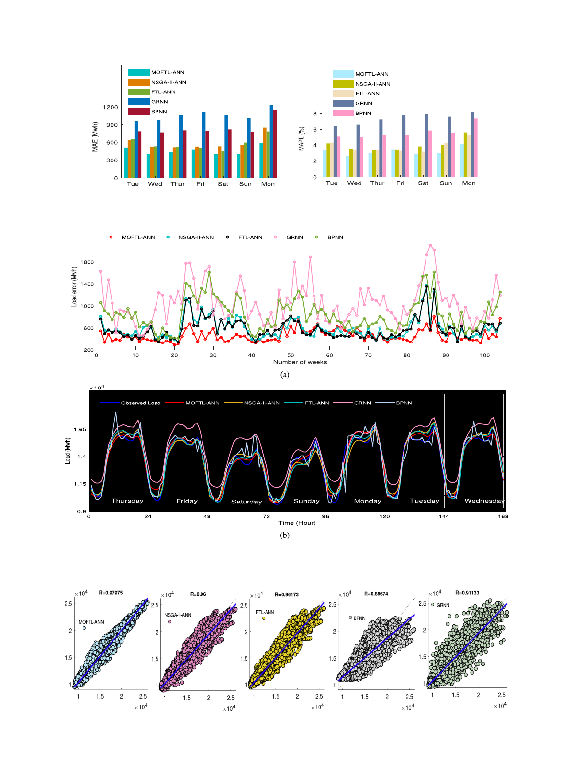
Fig. 7 shows the comparison of average MAE and MAPE value
P. Singh, P. Dwivedi / Energy 182 (2019) 606e622 613
Fig. 5. Obtained Pareto optimal solutions by MOFTL, MOWCA, MOPSO and NSGA-II for ZDT1. (Note: PF represents Pareto Font).
Fig. 6. Obtained Pareto optimal solutions by MOFTL, MOWCA, MOPSO and NSGA-II for ZDT3. (Note: PF represents Pareto Font).
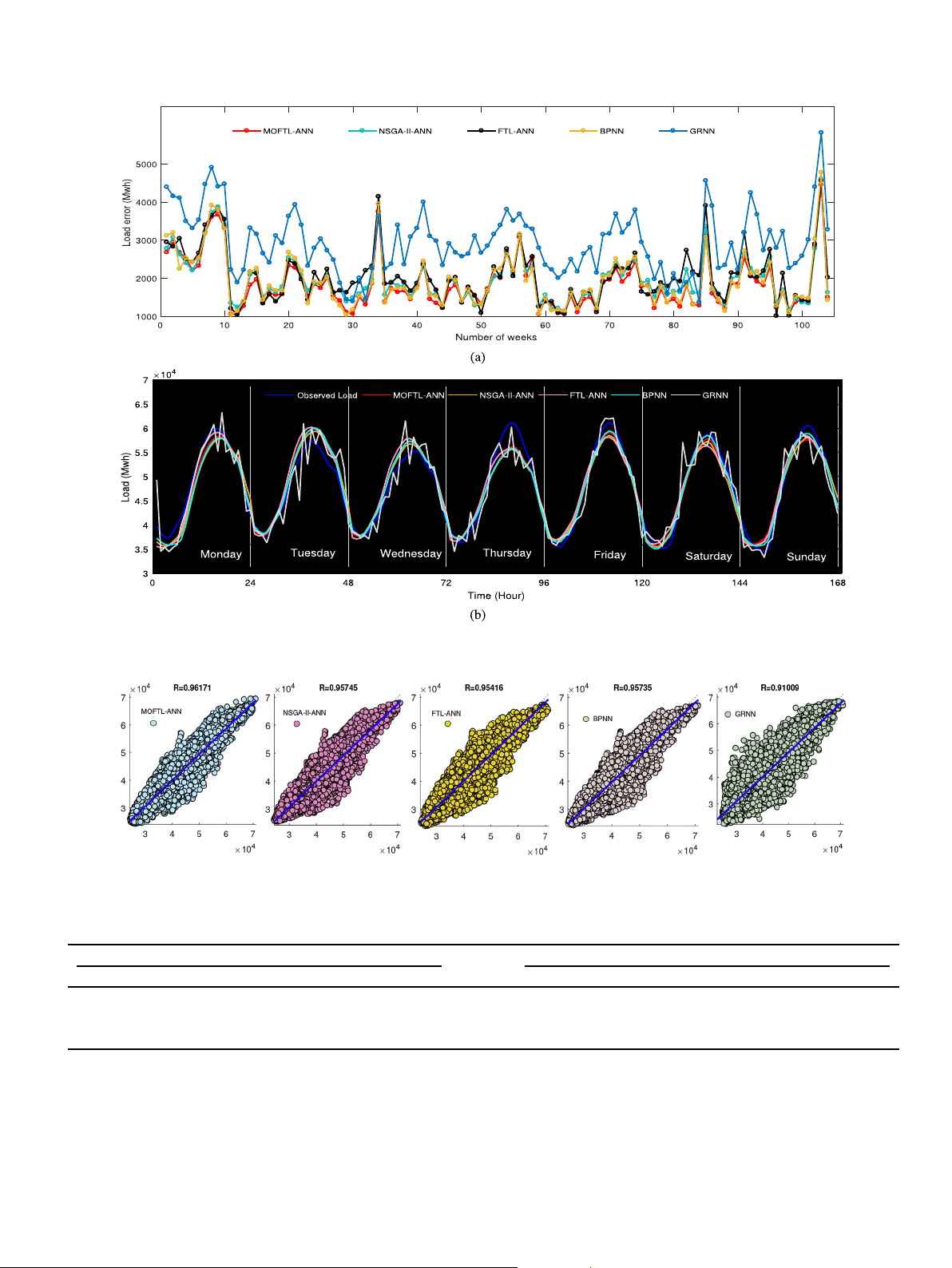
generated by all five forecasting model on a daily basis. The figure
objective functions at the same time. Fig. 8-a shows a comparison of
clearly shows that MOFTL-ANN generated least MAE on each day of
average weekly load error found during load prediction for years
the week while GRNN produced maximum MAE and MAPE. It can
2008e2009. The figure reveals that MOFTL established to draw
also be noted that MAPE generated on Friday by FTL-ANN is less
least average weekly load error in almost all weeks for the years
than that of MOFTL-ANN due to the limitation of solving two
2008 and 2009 while GRNN generated high peaks of average load 614
P. Singh, P. Dwivedi / Energy 182 (2019) 606e622 Table 3 Evaluation metrics. S.No. Metric Equation 1 Mean absolute error 1X n MAE ¼ y N j¼1 j y0j 2 Maximum error percentage ð y0j yjÞ MEP ¼ 100 yj
rffiffiffiffiffiffiffiffiffiffiffiffiffiffiffiffiffiffiffiffiffiffiffiffiffiffiffiffiffiffiffiffiffiffiffiffiffiffi 3 Root of mean squared error 1Xn RMSE ¼ ðy N j¼1 j y0 jÞ2 4 Normalized mean squared error 1 X X n 1 n NMSE ¼ ðy ðy D2 j y0j Þ2 , D2 ¼ j yÞ2 N j¼1 N 1 j¼1 5 Mean absolute percent error 1X y n j y0 j MAPE ¼ 100 N j¼1 yj 6
Daily peak mean absolute percent error 1 jmaxðTL Daily Peak MAPE ¼ m Þ maxðFLm Þj 100 N maxðTLmÞ P 7
Pearson's correlation coefficient n r ¼ j¼1ðyj yÞðy0j y0Þ
qffiffiffiffiffiffiffiffiffiffiffiffiffiffiffiffiffiffiffiffiffiffiffiffiffiffiffiffiffiffi P P n n j¼1ðyj yÞ2 j¼1ðy0j y0Þ2 8 9 8 Directional change 100 X < = N1 0; otherwise DC ¼ a N 1 j¼1
t , at ¼ : 1; if ðy0jþ1 yjÞðyjþ1 yjÞ > 0 ; P 9 Index of agreement N IA ¼ 1 j¼1ðyj yjÞ2 PNj¼1ðy0j yÞðyj yÞ2
Note: yj ¼ actual value of day j, y0j ¼ predicted value of day j, y ¼ mean of actual value, y0 ¼ mean of Predicted value, FLm ¼ forecast load value for every 24 h, TLm ¼ target
load for every 24 h, N ¼ number of elements in training data.
error during all the weeks of the testing period. Fig. 8-b shows the Table 5
comparison of load obtained after prediction by all five models with Experimental parameter values.
the observed load. This comparison illustrates that MOFTL-ANN Forecasting model Experimental parameter Value
achieves the most accurate prediction values and also load con- MOFTL-ANN MOFTL inertia weight 0.75
sumption during weekends is less compared to weekdays. Fig. 9
MOFTL maximum number of iterations 100
shows the relationship between observed and predicted load by MOFTL population size 50
all five forecasting models in which MOFTL-ANN show a strong NSGA-II-ANN GA crossover ratio 0.7 relation. GA mutation ratio 0.3 GA population size 50
Remark. From the obtained experimental results, MOFTL-ANN FTL-ANN Tolerance value 108
seems to be the most accurate hybrid model. These tables and FTL inertia weight 0.67
figures illustrate that our proposed hybrid model is the most su- GA population size 50
perior, accurate and stable forecasting model. BPNN Learning rate 0.1 GRNN Training precision 105 4.6. Case study-2: ERCOT
obtained result, it can be clearly noticed that MOFTL-ANN finds a 4.6.1. Data description
better optimal solution than other forecasting models. Evaluation
In this experiment, hourly load data set of ERCOT for the years
metrics like average values of MAE- 1891.478 Mwh, MEP- 31.145%,
2009e2014 have been taken as training data and years 2015e2016
RMSE- 2586.809 Mwh, NMSE- 0.077475 Mwh, MAPE- 4.811885%,
for testing purpose [66]. Table 6 shows the correlation between
Pearson correlation coefficient (r)- 0.9606 makes MOFTL-ANN su-
input variables and load taken into consideration. ALL the statistical
perior than other forecasting models. GRNN generates a minimum
parameters related to the ERCOT data set is shown in Table 4. Five
average directional change of 67.1173 while MOFTL-have maximum
parameters namely, an hour of the day, the day of the week, 168-hr - 71.8093.
lagged load, 24-hr lagged load and previous 24-hr average load has
Table 11 and Table 12 shows month wise MAE and MAPE error
been chosen for load prediction of ERCOT region.
values of all five forecasting models. The table compares the result
obtained from the experiment and found that MOFTL-ANN gener- 4.6.2. Results
ates superior result. Very exceptionally, it can be noted that for the
Table 10 shows the minimu, average and maximum values of all
month Dec 2015, FTL-ANN generated lesser MAPE of 4.44200%
the forecasting models namely, MOFTL-ANN, NSGA-II-ANN, FTL-
while MAPE of MOFTL-ANN is 4.9073%. The reason for this
ANN, BPNN, and GRNN for the years 2015 and 2016. From the Table 4
Statistical parameters for the data used in this paper. Region Samples # of elements Mean Max Median Min Std. ISO New Pool England All 52608 15093.259 28130 15277 9040 2958.703 Training 35064 15270.068 28130 15473 9152 3007.685 Testing 17544 14739.883 26111 14982 9040 2825.413 ERCOT All 70128 37865.985 71092.609 35656.533 21378.730 9260.466 Training 52584 37208.379 68317.669 34917.492 21378.730 9155.398 Testing 17544 39837.002 71092.609 37625.894 24337.467 9294.055
P. Singh, P. Dwivedi / Energy 182 (2019) 606e622 615 Table 6
phenomena is likely that FTL-ANN is a single-objective model
Correlation coefficient (r) between input parameters and the load data sets.
which can handle trends and randomness while MOFTL-ANN is a Input parameter r r
multi-objective model and it has to handle both accuracy and sta- bility simultaneously. (ISO) (ERCOT)
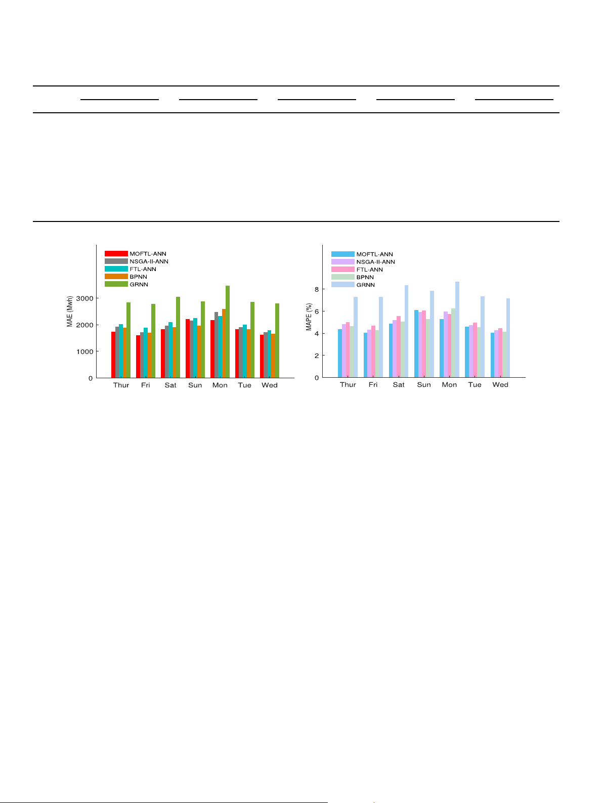
The comparison of average MAE and MAPE value generated by Dry Bulb Temperature 0.19 e
all five forecasting model on a daily basis is shown in Fig. 10. The Dew Point Temperature 0.07 e Hour of the Day 0.51 0.3418
figure clearly shows that MOFTL-ANN generated least MAE on each Day of the Week 0.03 0.0062
day of the week except Sunday, BPNN produced minimum MAE.
Holiday/Weekend indicator (0 or 1) 0.26 e
Similarly, on Sunday and Tuesday, MAPE of BPNN is less than
168-hr (previous week) Lagged Load 0.85 0.82
MOFTL-ANN. The reason for such a situation lies in the nonlinear 24-hr Lagged Load 0.90 0.94
behavior of data trends. GRNN produced maximum MAE and MAPE Previous 24-hr Average Load 0.56 0.7477
on each day that proves its unsuitability for load prediction. Fig. 11-
a shows a comparison of average weekly load error for the year Table 7
Forecasting results of the five forecasting models. Forecasting Models MAE MEP RMSE NMSE MAPE Daily peak MAPE r DC IA MOFTL-ANN Min 457.8729 11.49369 597.0174 0.044649 3.201904 2.504589 0.969801 72.55316 0.983564 Avg 504.1671 15.26862 655.7201 0.054012 3.496752 3.03031 0.974153 73.87733 0.988558 Max 547.7367 19.60747 711.1898 0.063359 3.828821 3.499827 0.979748 74.77056 0.986071 NSGA-II-ANN Min 582.4166 19.3054 779.6671 0.076147 3.92285 3.631563 0.952252 69.86832 0.96693 Avg 629.1621 20.92272 840.1871 0.088878 4.234364 4.094272 0.957317 70.9776 0.976367 Max 780.1065 24.75158 1001.752 0.125706 5.13332 6.045748 0.961517 72.08573 0.979975 FTL-ANN Min 523.3067 17.02067 692.2375 0.060027 3.543245 3.205244 0.959864 70.89437 0.979468 Avg 553.2902 19.94162 741.0733 0.068972 3.75242 3.675925 0.965272 72.49957 0.984357 Max 601.5597 22.40104 795.0949 0.079191 4.126287 3.940751 0.970286 73.98963 0.982063 BPNN Min 458.1641 16.82907 594.3669 0.044253 3.07581 2.648605 0.886737 62.68027 0.9298 Avg 579.5099 20.58969 775.7784 0.080456 3.919104 3.711811 0.959404 72.55772 0.977829 Max 1057.095 28.75839 1326.469 0.22041 7.345048 6.091889 0.979059 75.22659 0.988835 GRNN Min 624.5459 19.41066 859.5813 0.092557 4.21692 4.155094 0.911327 55.56632 0.559852 Avg 1199.392 29.77542 1542.116 0.328479 8.676287 7.147476 0.9415 62.11993 0.825696 Max 1812.585 36.30503 2285.68 0.654436 13.451 10.41273 0.953108 70.48965 0.974442 Table 8
Comparing monthly MAPE and MAE of the five forecasting models for years 2008. Month MOFTL-ANN NSGA-II-ANN FTL-ANN BPNN GRNN MAPE MAE MAPE MAE MAPE MAE MAPE MAE MAPE MAE Jan 2.755553 432.0074 3.772639 596.9734 3.582295 572.7084 5.525351 873.5551 7.229363 1178.512 Feb 2.708985 418.9039 3.138612 492.1177 2.980873 465.5721 5.680188 874.2147 5.448159 873.442 Mar 2.732399 393.22 3.79806 556.9457 3.05918 455.8828 4.905664 718.3088 3.640049 538.5853 Apr 2.727465 357.6796 3.464602 467.4888 3.19827 441.2072 4.056142 547.9548 7.78487 993.6697 May 2.628354 337.0947 3.29717 442.3028 3.233623 435.7069 3.474783 467.7393 8.615562 1065.285 Jun 3.369919 524.8216 5.553908 902.2284 5.28079 858.8203 7.778607 1262.292 8.850961 1459.154 July 2.98754 494.6581 4.945192 841.1846 4.74118 810.5707 7.668619 1318.876 7.755603 1381.83 Aug 2.497684 380.4252 4.308996 669.0496 4.199161 656.5596 6.241044 970.9933 5.466167 847.0691 Sept 3.082095 447.0101 4.532354 678.9162 4.434905 656.2067 6.373994 953.5084 8.372256 1206.877 Oct 2.583371 339.3431 2.866891 384.2469 3.053968 413.2177 3.693108 507.0441 6.57141 822.9664 Nov 3.219481 443.9945 3.580922 511.5356 3.926719 566.2431 6.0355 863.6141 6.522948 902.2965 Dec 3.968775 591.79 4.712281 715.2392 4.797472 732.7311 7.142112 1084.901 7.986139 1235.85 Table 9
Comparing monthly MAPE and MAE of the five forecasting models for years 2009. Month MOFTL-ANN NSGA-II-ANN FTL-ANN BPNN GRNN MAPE MAE MAPE MAE MAPE MAE MAPE MAE MAPE MAE Jan 3.551231 563.8089 3.286316 519.4472 3.287094 515.5938 5.696559 907.8121 8.251354 1354.426 Feb 3.573261 529.6609 3.559469 523.3133 3.342885 494.7484 5.496871 821.9467 5.333443 811.9557 Mar 4.195243 582.9211 3.915231 550.3764 3.338061 469.4018 5.03026 703.6413 6.178395 840.7755 Apr 3.742518 467.2049 3.965368 518.8956 3.509731 467.4801 4.864393 651.1306 8.555542 1049.714 May 3.52047 438.5759 3.532622 450.0189 3.220264 410.7452 5.18462 688.4336 9.541995 1133.21 Jun 3.055679 403.5158 3.156944 435.0509 3.493532 471.0829 4.262338 601.0097 6.238585 773.3182 July 2.746453 402.1409 4.059018 624.9799 4.089833 625.374 5.524043 858.5648 7.298816 1102.566 Aug 3.987541 637.3829 6.488447 1079.202 6.390219 1053.221 8.614247 1414.386 10.59996 1776.406 Sept 3.30444 442.0353 4.27097 587.1466 4.166079 568.5463 5.503848 761.8917 9.15875 1183.251 Oct 3.197969 410.5056 3.287985 439.7042 3.302124 447.0866 4.585281 632.3976 7.313592 902.4808 Nov 3.206459 411.9029 3.720922 506.2413 4.178728 566.2651 4.683497 641.6848 6.120391 747.6338 Dec 3.509934 537.4623 3.78914 588.6671 4.063178 626.7831 6.684146 1030.1 7.221532 1148.9 616
P. Singh, P. Dwivedi / Energy 182 (2019) 606e622
Fig. 7. Comparison of MAE and MAPE of five forecasting models.
Fig. 8. Comparison of observed load with forecast load by five forecasting models.
Fig. 9. Relationship between observed load and forecasted load by five forecasting models for England region.
P. Singh, P. Dwivedi / Energy 182 (2019) 606e622 617 Table 10
Forecasting results of the five forecasting models for years 2015 and 2016. Forecasting Models MAE MEP RMSE NMSE MAPE Daily peak MAPE r DC IA MOFTL-ANN Min 1856.41 28.5497 2548.873 0.075212 4.735964 4.974963 0.959558 71.07108 0.979343 Avg 1891.478 31.1451 2586.809 0.077475 4.811885 5.09004 0.960604 71.80927 0.979783 Max 1918.213 32.58433 2624.876 0.079764 4.880519 5.231137 0.961706 72.37645 0.980342 NSGA-II-ANN Min 1921.28 32.07367 2627.326 0.079913 4.890396 5.122149 0.955678 68.43185 0.977111 Avg 1977.051 33.03538 2686.517 0.083565 5.022934 5.310469 0.957391 70.02856 0.977918 Max 2026.914 33.78354 2737.688 0.086768 5.165887 5.566259 0.959283 70.84877 0.979093 FTL-ANN Min 1973.962 32.93888 2681.217 0.083225 4.981819 5.324419 0.956565 69.51491 0.977315 Avg 1984.522 33.45472 2700.732 0.084443 5.020921 5.4492 0.956922 69.99658 0.977613 Max 1993.758 33.78354 2711.276 0.085101 5.066037 5.566259 0.957538 70.55806 0.978027 BPNN Min 1825.277 28.82691 2581.392 0.077143 4.630577 4.658941 0.953929 69.361 0.97624 Avg 1924.832 32.64605 2687.813 0.083703 4.867707 5.228421 0.957728 71.13037 0.978355 Max 2037.037 36.59138 2806.018 0.091153 5.146417 5.888341 0.961168 72.05723 0.980269 GRNN Min 2051.709 31.04214 2786.324 0.089878 5.294412 5.138398 0.91009 64.43026 0.95337 Avg 2405.141 32.18474 3156.274 0.116847 6.15749 6.838773 0.943329 67.11737 0.967091 Max 2948.473 36.05517 3958.327 0.18139 7.697825 8.62503 0.954116 69.89112 0.976004 Table 11
Comparing monthly MAPE and MAE of the five forecasting models for year 2015. Month MOFTL-ANN NSGA-II-ANN FTL-ANN BPNN GRNN MAPE MAE MAPE MAE MAPE MAE MAPE MAE MAPE MAE Jan 6.557777 2553.352 6.533426 2557.057 6.976802 2692.852 6.641719 2627.534 10.11026 3892.244 Feb 7.938058 3114.914 8.188373 3210.021 8.286305 3231.942 8.240336 3277.947 11.06183 4177.604 Mar 5.276459 1877.585 5.872915 2061.94 5.784634 2055.804 5.406229 1934.96 8.527302 2941.973 Apr 4.854562 1681.776 5.389833 1877.843 5.112522 1773.487 5.42361 1910.289 8.305066 2859.087 May 5.320253 2037.666 5.615279 2171.024 5.395839 2068.965 5.763074 2240.157 9.326754 3504.155 Jun 3.881549 1753.297 4.016854 1833.068 4.165233 1862.719 3.840786 1760.432 6.108553 2731.761 July 2.709052 1309.892 3.2211 1561.669 3.622653 1766.392 2.642116 1297.729 3.780322 1850.192 Aug 4.282922 2027.395 4.789138 2257.121 5.286263 2528.499 4.369791 2088.256 4.987809 2341.532 Sept 3.839865 1621.875 4.099053 1749.562 4.451325 1887.003 3.854501 1669.951 6.508854 2785.239 Oct 4.682193 1669.414 4.929145 1755.113 5.1547 1853.345 4.78041 1738.486 8.881864 3203.972 Nov 4.789588 1615.619 5.00434 1700.246 5.006814 1696.372 5.104504 1741.555 7.988978 2678.502 Dec 4.756019 1659.083 4.442005 1558.45 4.730951 1656.413 4.582497 1616.409 8.516669 2945.617
2015e2016. It can be clearly seen that average weekly load gener-
of two or more forecasting models [67]. The statistic F of the
ated for the years 2015 and 2016 by MOFTL-ANN is minimum for Friedman test is shown as
most of the weeks while GRNN seems to generate high peaks " #
during all the weeks of the testing period. Fig. 11-b shows the 12N X q qðq þ 1Þ2 F ¼ Rank2 (8)
comparison of the actual load with the load predicted by all five qðq þ 1Þ j 4 j¼1
forecasting models. This comparison illustrates that MOFTL-ANN
achieves the most accurate prediction values than any other
where N is the total number of forecasting results; q is a number of
compared forecasting models. Fig. 12 shows a strong relationship
forecasting models compared; Rank
between observed and predicted load than other forecasting j is the average rank sum
received from each forecasting value for each model. The null hy- models.
pothesis for Friedman's test is all compared forecasting models
Remark. From all the experimental results shown in this case
generate same forecasting errors and the alternative hypothesis is
study, it can be clearly stated that MOFTL-ANN can enhance accu-
the negation of the null hypothesis.
racy and stability. Also, these results illustrate that our proposed
In this paper, the Friedman test is implemented under a ¼ 0:05
hybrid model is superior to other mentioned forecasting models.
significance level. The results shown in Table 13 by the Friedman
test shows that forecasting results of all forecasting models are 5. Discussions
different. At a ¼ 0:05, the null hypothesis fails and the result shows
that every state-of-the-art model generates a unique forecasting
In this section, some insightful discussions for the experimental result.
results obtained are provided with more details.
5.2. Stability of the forecasting models
5.1. The significance of MOFTL-ANN: based on the Friedman statistical test
Error reduction in load forecasting is an important aspect of
showing the performance of forecasting models but the model
This subsection further compares the forecasting abilities of the
considering both accuracy and stability is preferred most. Thus, in
proposed hybrid model with the compared forecasting models by
this paper, the standard deviation is utilized to evaluate the sta-
using the Friedman statistical test.
bility of the hybrid model and comparison models. Additionally, the
The Friedman test is a non-parametric, multiple comparisons
error metrics MAE and NMSE are the most important indicators
test that aims to detect significant differences between the results
used to evaluate the performance of forecasting models. The 618
P. Singh, P. Dwivedi / Energy 182 (2019) 606e622 Table 12
Comparing monthly MAPE and MAE of the five forecasting models for the year 2016. Month MOFTL-ANN NSGA-II-ANN FTL-ANN BPNN GRNN MAPE MAE MAPE MAE MAPE MAE MAPE MAE MAPE MAE Jan 6.770209 2504.269 6.86443 2535.682 6.911179 2542.062 6.698792 2503.021 10.01666 3652.253 Feb 4.842234 1668.319 4.863737 1671.066 5.009048 1730.429 4.616692 1604.06 7.969788 2682.616 Mar 3.696451 1218.768 3.875041 1288.495 3.838115 1273.992 3.820356 1280.707 6.885492 2267.139 Apr 4.330271 1543.283 4.614292 1658.886 4.432312 1586.132 4.614475 1672.083 7.843856 2755.391 May 5.574658 2160.955 5.923943 2306.216 5.977383 2331.081 6.001755 2371.869 9.070539 3475.827 Jun 3.551048 1622.904 3.902762 1793.313 3.783588 1713.914 3.677367 1694.641 5.400061 2442.063 July 2.96804 1473.355 3.543854 1762.451 4.270406 2167.944 2.999465 1516.806 3.808573 1921.726 Aug 3.757903 1789.257 4.233035 2033.697 4.785633 2313.383 3.826978 1869.077 6.160521 2886.897 Sept 4.344463 1886.302 4.714515 2039.427 5.173031 2238.765 4.326536 1898.989 6.374026 2767.847 Oct 4.88653 1918.785 5.297524 2083.694 5.188784 2036.36 5.05911 2026.186 8.842943 3376.523 Nov 4.045829 1353.42 4.157906 1400.24 4.399363 1495.028 4.203166 1429.131 7.613245 2588.779 Dec 6.444455 2497.858 6.495171 2524.576 6.956649 2678.913 6.704293 2632.203 10.74334 4032.632
Fig. 10. Comparison of MAE and MAPE of five forecasting models.
smaller the standard deviation is, the stronger the stability will be.
MOFTL-ANN forecasting model is less that NSGA-II-ANN and GRNN.
Table 14 shows the statistical values of MAE and NMSE for by
However, the computation time of the proposed algorithm
five forecasting models over 50 iterations. MOFTL-ANN yields best
(MOFTL) and proposed hybrid model (MOFTL-ANN) is little longer
statistical values such as a minimum MAE value of 457.8729,
than some of the comparison models, but this seems justified due
maximum MAE of 547.7367, an average MAE value of 504.1671 and
to its superior forecasting abilities. Further this computation time
standard deviation of 547.7367 while other forecasting models
can be minimized by using a high-performance systems.
yielded higher statistical values than our proposed hybrid model
for case study 1. Table also reveals that NMSE statistical values of
MOFTL-ANN have lower values than other forecasting models for 5.4. Summary
case study 1. The statistics show that MAE and NMSE of MOFTL-
ANN yields the least standard deviation of 23.0549 and 0.001633
Based on the analysis drawn from experiment- I, experiment- II respectively for case study 2.
and the discussions above, the following conclusions can be drawn:
Tabular results obtained show that MOFTL-ANN is superior to
The proposed hybrid forecasting model based on MOFTL has very
compared forecasting models. Therefore, we can conclude that
strong forecasting ability and more stable forecasting results than
MOFTL-ANN achieves the desirable forecasting stability, is more
FTL-ANN, NSGA-II-ANN, BPNN, and GRNN.
stable than other compared models and can be an effective tech-
nique for electricity load forecasting in the real electricity market.
MOFTL optimization algorithm outperforms MOWCA, MOPSO,
and NSGA-II over multi-objective test functions. Also, MOFTL 5.3. Run time
has shorter computation time values of 178.747056 s, 157.5818 s,
147.469428 s, 165.879441 s for FON, SCH, ZDT1 and ZDT3 multi-
All the experiments are performed in the MATLAB R2017a
objective test functions over MOWCA and NSGA-II.
software on a Windows 10, 64-bit machine with Intel(R) Core(TM)
MOFTL-ANN, a hybrid model enhanced the load forecasting
i5 CPU 760 @ 2.80 GHz with 1 processor.
accuracy by improving the forecasting ability of ANN. The pro-
Table 15 and Table 16 shows the computation time in seconds
posed hybrid model shows improvement of 17.42%, 6.81%,
obtained from experiment 1 and experiment 2. It can be observed
10.77% and 59.69% MAPE values for England region and 4.20%,
that the running time of MOFTL is 178.747056 s, 157.5818 s,
4.16%, 1.14% and 21.85% MAPE values for ERCOT region over
147.469428s and 165.879441 s for FON, SCH, ZDT1 and ZDT3 in
NSGA-II-ANN, FTL-ANN, BPNN, and GRNN forecasting models.
Experiment I and 1485.315609 s and 1698.172034 s in Experiment
Results from Friedman statistical test show that all compared
II. This show that the computation time of MOFTL is shorter than
forecasting models generate different forecasting results.
MOWCA and NSGA-II and demonstrates that it can find Pareto
Moreover, standard deviation values of 0.006027 and 0.001633
optimal solutions in less time. Similarly, the computation time of
for England region and ERCOT region by the proposed hybrid
P. Singh, P. Dwivedi / Energy 182 (2019) 606e622 619
Fig. 11. Comparison of observed load with forecast load by five forecasting models.
Fig. 12. Relationship between observed load and forecasted load by five forecasting models for the ERCOT region. Table 13
Results of Friedman test for Experiment II. Compared Models Significant level (a ¼ 0:05) Compared Models Significant level (a ¼ 0:05) Case Study I Case Study II MOFTL-ANN vs. NSGA-II-ANN
H0 : e1 ¼ e2 ¼ e3 ¼ e4 ¼ e5 MOFTL-ANN vs. NSGA-II-ANN
H0 : e1 ¼ e2 ¼ e3 ¼ e4 ¼ e5 MOFTL-ANN vs. FTL-ANN F ¼ 8470.368 MOFTL-ANN vs. FTL-ANN F ¼ 3368.516 MOFTL-ANNR vs. BPNN P ¼ 0.00000 (Reject H0) MOFTL-ANNR vs. BPNN P ¼ 0.00000 (Reject H0) MOFTL-ANN vs. GRNN MOFTL-ANN vs. GRNN
model is least compared to other forecasting models which
MOFTL-ANN, it can be considered as a new viable option for
describe that MOFTL-ANN is the most stable one.
time series forecasting abilities.
A novel multi-objective optimization algorithm, namely MOFTL,
outperforms MOWCA, MOPSO, and NSGA-II and it adds a new
Remark. Compared to the state-of-the-art models, MOFTL-ANN
optimization algorithm for solving multi-objective optimization
generates better results for experiment-I and experiment- II based
problems. Due to high accuracy and stable load forecasting by
on evaluation criteria. On the basis of obtained results, we can 620
P. Singh, P. Dwivedi / Energy 182 (2019) 606e622 Table 14
Statistical values of MAE and NMSE obtained from forecasting results of England and ERCOT region by forecasting models. Experiment II Forecasting model MAE NMSE Case Study - 1 Min Max Avg Std Min Max Avg Std MOFTL-ANN 457.8729 547.7367 504.1671 27.50089 0.044649 0.063359 0.054012 0.006027 NSGA-II-ANN 582.4166 780.1065 629.1621 57.21251 0.076147 0.125706 0.088878 0.014146 FTL-ANN 523.3067 601.5597 553.2902 27.89063 0.060027 0.079191 0.068972 0.007396 BPNN 458.1641 1057.095 579.5099 177.1325 0.044253 0.22041 0.080456 0.051533 GRNN 624.5459 1812.585 1199.392 437.0547 0.092557 0.654436 0.328479 0.206532 Experiment II MOFTL-ANN 1856.41 1918.213 1891.478 23.05498 0.075212 0.079764 0.077475 0.001633 Case Study - 2 NSGA-II-ANN 1921.28 13876.34 3166.98 3762.978 0.079913 2.313992 0.306608 0.705325 FTL-ANN 2050.343 8963.795 6646.426 2081.043 0.090739 1.401217 0.85099 0.413967 BPNN 1825.277 2037.037 1924.832 72.61513 0.077143 0.091153 0.083703 0.005043 GRNN 2051.709 2948.473 2405.141 310.9689 0.089878 0.18139 0.116847 0.029389 Table 15
To achieve such forecasting model, a novel multi-objective
Computation time (seconds) of multi-objective algorithms over FON, SCH, ZDT1 and
optimization algorithm MOFTL have been proposed and com- ZDT2 test functions.
bined with the artificial neural network to optimize weights. To Models FON SCH ZDT1 ZDT3
verify the performance of the proposed hybrid model, nine per- MOFTL 178.747056 157.5818 147.469428 165.879441
formance evaluation metrics including MAE, MEP, RMSE, NMSE, MOWCA 191.321965 260.145963 229.378474 223.891435
MAPE, Pearson's correlation coefficient, DC and IA have been used MOPSO 58.09828 68.715269 67.32384 54.446691
in this paper. Based on the series of results drawn from experiment NSGA-II 227.947349 207.794532 162.985784 162.985784
II, the performance of our proposed hybrid model over two data
sets shows that MOFTL-ANN is capable of predicting load with
higher accuracy and effective stability. Experiment II shows the Table 16
effectiveness of the proposed hybrid models over compared models
Computation time (seconds) of multi-objective algorithms over case study - 1 and
for electricity load forecast. In both the case study, MOFTL generates case study - 2.
superior results than NSGA-II-ANN, FTL-ANN, BPNN, and GRNN for Models Case Study I Case Study II
all performance evaluation indexes with lesser computation time. MOFTL-ANN 1485.315609 1698.172034
MOFTL-ANN shows improvement of 17.42%, 6.81%, 10.77% and NSGA-II-ANN 2477.819376 2866.610707
59.69% MAPE values over NSGA-II-ANN, FTL-ANN, BPNN and GRNN FTL-ANN 1137.724773 2978.105397
for England region and 4.20%, 4.16%, 1.14% and 21.85% MAPE values BPNN 524.8064923 399.106586
over NSGA-II-ANN, FTL-ANN, BPNN and GRNN for ERCOT region. GRNN 3600.839397 3162.42325
deduce that the MOFTL, can be used for solving multi-objective
optimization problems. Additionally, MOFTL-ANN is a robust, Abbreviations
highly accurate and stable hybrid model which can be used as a practical forecasting model. ACO Ant Colony Optimization ANN Artificial Neural Network BPNN Backpropagation Neural Network
5.5. Real applications, limitations and future work DC Directional Change DE Differential Evolutionary
The proposed forecasting model can contribute to the electricity ERCOT
Electric Reliability Council of Texas
market in dealing with future changes in load generation and FTL Follow The leader
transmission. It can be used for many real applications such as wind GA Genetic Algorithm
energy forecasting, hydro energy forecasting that are based on time GRNN
Generalized Regression Neural Network
series forecasting as the proposed hybrid forecasting model shows IA Index of Agreement
better ability to predict the future load with better accuracy and MAE Mean Absolute Error
stability. There are still some issues that must be resolved in future MEP Maximum Error Percentage
studies: load affecting factors such as rainfall and wind speed can MAPE Mean Absolute Percentage Error
be considered for more reliable and practical forecasting; advanced MOALO
Multi-Objective Ant Lion Optimizer
data pre-processing method can improve the forecasting results. MOFA
Multi-Objective Firefly Algorithm MOFPA
Multi-Objective Flower Pollination Algorithm 6. Conclusions MOFTL
Multi-Objective Follow The Leader MOP Multi-Objective Problem
Higher accuracy and excellent stability in electricity load fore- MOPSO
Multi-Objective Particle Swarm Optimization
casting play a very important role in the operation of power sys- MOWCA
Multi-objective Water Cycle Algorithm
tems. This paper provides a great tool for energy providers to know MOWOA
Multi-Objective Whale Optimization Algorithm
the amount of load demand in a particular region. The results NSGA-II Non-dominated Sorting GA
achieved from forecasting models show that our proposed hybrid NMSE Normalized Mean Squared Error
model results in outstanding forecasting performance. It is highly PSO Particle Swarm Optimization
desirable to develop a model that enhances both accuracy and RMSE Root Mean Squared Error stability simultaneously. SVM Support Vector Machine
P. Singh, P. Dwivedi / Energy 182 (2019) 606e622 621 References
[32] Kavousi-Fard A, Samet H, Marzbani F. A new hybrid modified firefly algorithm
and support vector regression model for accurate short term load forecasting.
Expert Syst Appl 2014;41(13):6047e56.
[1] Xiao L, Shao W, Wang C, Zhang K, Lu H. Research and application of a hybrid
[33] Xiao L, Qian F, Shao W. Multi-step wind speed forecasting based on a hybrid
model based on multi-objective optimization for electrical load forecasting.
forecasting architecture and an improved bat algorithm. Energy Convers Appl Energy 2016;180:213e33. Manag 2017;143:410e30.
[2] Almeshaiei E, Soltan H. A methodology for electric power load forecasting.
[34] Bashir Z, El-Hawary M. Applying wavelets to short-term load forecasting
Alexandria Eng J 2011;50(2):137e44.
using pso-based neural networks. IEEE Trans Power Syst 2009;24(1):20e7.
[3] Hahn H, Meyer-Nieberg S, Pickl S. Electric load forecasting methods: Tools for
[35] Liao G-C, Tsao T-P. Application of a fuzzy neural network combined with a
decision making. Eur J Oper Res 2009;199(3):902e7.
chaos genetic algorithm and simulated annealing to short-term load fore-
[4] Tucci M, Crisostomi E, Giunta G, Raugi M. A multi-objective method for short-
casting. IEEE Trans Evol Comput 2006;10(3):330e40.
term load forecasting in european countries. IEEE Trans Power Syst
[36] Hong W-C. Electric load forecasting by seasonal recurrent svr (support vector 2016;31(5):3537e47.
regression) with chaotic artificial bee colony algorithm. Energy 2011;36(9):
[5] D. Bunn, E. D. Farmer, Comparative models for electrical load forecasting. 5568e78.
[6] Amjady N. Short-term hourly load forecasting using time-series modeling
[37] Kouhi S, Keynia F, Ravadanegh SN. A new short-term load forecast method
with peak load estimation capability. IEEE Trans Power Syst 2001;16(4):
based on neuro-evolutionary algorithm and chaotic feature selection. Int J 798e805.
Electr Power Energy Syst 2014;62:862e7.
[7] Li S, Wang P, Goel L. A novel wavelet-based ensemble method for short-term
[38] Yang Y, Chen Y, Wang Y, Li C, Li L. Modelling a combined method based on
load forecasting with hybrid neural networks and feature selection. IEEE Trans
anfis and neural network improved by de algorithm: A case study for short- Power Syst 2016;31(3):1788e98.
term electricity demand forecasting. Appl Soft Comput 2016;49:663e75.
[8] Abedinia O, Amjady N, Zareipour H. A new feature selection technique for load
[39] Meng X, Chang J, Wang X, Wang Y. Multi-objective hydropower station
and price forecast of electrical power systems. IEEE Trans Power Syst
operation using an improved cuckoo search algorithm. Energy 2019;168: 2017;32(1):62e74. 425e39.
[9] Ceperic E, Ceperic V, Baric A. A strategy for short-term load forecasting by
[40] Zhang X, Wang J. A novel decomposition-ensemble model for forecasting
support vector regression machines. IEEE Trans Power Syst 2013;28(4):
short-term load-time series with multiple seasonal patterns. Appl Soft Com- 4356e64. put 2018;65:478e94.
[10] Ahmad T, Chen H. Potential of three variant machine-learning models for
[41] Goel R, Maini R. A hybrid of ant colony and firefly algorithms (hafa) for solving
forecasting district level medium-term and long-term energy demand in
vehicle routing problems. J Comput Sci 2018;25:28e37.
smart grid environment. Energy 2018;160:1008e20.
[42] Bao C, Xu L, Goodman ED, Cao L. A novel non-dominated sorting algorithm for
[11] Xiao L, Shao W, Liang T, Wang C. A combined model based on multiple sea-
evolutionary multi-objective optimization. J Comput Sci 2017;23:31e43.
sonal patterns and modified firefly algorithm for electrical load forecasting.
[43] Banati H, Chaudhary R. Multi-modal bat algorithm with improved search Appl Energy 2016;167:135e53.
(mmbais). J Comput Sci 2017;23:130e44.
[12] P. Singh, P. Dwivedi, V. Kant, A hybrid method based on neural network and
[44] Deb K, Pratap A, Agarwal S, Meyarivan T. A fast and elitist multiobjective
improved environmental adaptation method using controlled Gaussian mu-
genetic algorithm: Nsga-ii. IEEE Trans Evol Comput 2002;6(2):182e97.
tation with real parameter for short-term load forecasting, Energy.
[45] Deb K. Multi-objective optimization using evolutionary algorithms, vol. 16.
[13] Singh P, Mishra K, Dwivedi P. Enhanced hybrid model for electricity load John Wiley & Sons; 2001.
forecast through artificial neural network and jaya algorithm. In: 2017 In-
[46] Deb K. Multi-objective optimization. In: Search methodologies. Springer;
ternational Conference on intelligent computing and control systems (ICICCS), 2014. p. 403e49. IEEE; 2017. p. 115e20.
[47] Du P, Wang J, Guo Z, Yang W. Research and application of a novel hybrid
[14] Liao G-C, Tsao T-P. Application of fuzzy neural networks and artificial intel-
forecasting system based on multi-objective optimization for wind speed
ligence for load forecasting. Electr Power Syst Res 2004;70(3):237e44.
forecasting. Energy Convers Manag 2017;150:90e107.
[15] Liang R-H, Cheng C-C. Short-term load forecasting by a neuro-fuzzy based
[48] Ali E, Elazim SA, Abdelaziz A. Ant lion optimization algorithm for renewable
approach. Int J Electr Power Energy Syst 2002;24(2):103e11.
distributed generations. Energy 2016;116:445e58.
[16] Lou CW, Dong MC. Modeling data uncertainty on electric load forecasting
[49] Xiao L, Shao W, Yu M, Ma J, Jin C. Research and application of a combined
based on type-2 fuzzy logic set theory. Eng Appl Artif Intell 2012;25(8):
model based on multi-objective optimization for electrical load forecasting. 1567e76. Energy 2017;119:1057e74.
[17] Chen B-J, Chang M-W, et al. Load forecasting using support vector machines:
[50] Wang J, Du P, Niu T, Yang W. A novel hybrid system based on a new proposed
A study on eunite competition 2001. IEEE Trans Power Syst 2004;19(4):
algorithmemulti-objective whale optimization algorithm for wind speed 1821e30.
forecasting. Appl Energy 2017;208:344e60.
[18] Yan X, Chowdhury NA. Mid-term electricity market clearing price forecasting:
[51] Lokeshgupta B, Sivasubramani S. Multi-objective dynamic economic and
A multiple svm approach. Int J Electr Power Energy Syst 2014;58:206e14.
emission dispatch with demand side management. Int J Electr Power Energy
[19] Panigrahi S, Behera HS. A hybrid etseann model for time series forecasting. Syst 2018;97:334e43.
Eng Appl Artif Intell 2017;66:49e59.
[52] Deb K. Multi-objective optimization using evolutionary algorithms: An
[20] Guan C, Luh PB, Michel LD, Chi Z. Hybrid kalman filters for very short-term
introduction, Multi-objective evolutionary optimisation for product design
load forecasting and prediction interval estimation. IEEE Trans Power Syst
and manufacturing. 2011. p. 1e24. 2013;28(4):3806e17.
[53] Sadollah A, Eskandar H, Bahreininejad A, Kim JH. Water cycle algorithm for
[21] Hu Z, Bao Y, Xiong T, Chiong R. Hybrid filterewrapper feature selection for
solving multi-objective optimization problems. Soft Comput 2015;19(9):
short-term load forecasting. Eng Appl Artif Intell 2015;40:17e27. 2587e603.
[22] Haida T, Muto S. Regression based peak load forecasting using a trans-
[54] King AJ, Wilson AM, Wilshin SD, Lowe J, Haddadi H, Hailes S, Morton AJ.
formation technique. IEEE Trans Power Syst 1994;9(4):1788e94.
Selfish-herd behaviour of sheep under threat. Curr Biol 2012;22(14):R561e2.
[23] Hong T, Gui M, Baran ME, Willis HL. Modeling and forecasting hourly electric
[55] Lee K, Cha Y, Park J. Short-term load forecasting using an artificial neural
load by multiple linear regression with interactions. In: IEEE PES general
network. IEEE Trans Power Syst 1992;7(1):124e32. Meeting. IEEE; 2010. p. 1e8.
[56] Chen S-T, Yu DC, Moghaddamjo AR. Weather sensitive short-term load fore-
[24] Taylor JW. Short-term load forecasting with exponentially weighted methods.
casting using nonfully connected artificial neural network. IEEE Trans Power
IEEE Trans Power Syst 2012;27(1):458e64. Syst 1992;7(3):1098e105.
[25] Cho M, Hwang J, Chen C. Customer short term load forecasting by using arima
[57] Hippert HS, Pedreira CE, Souza RC. Neural networks for short-term load
transfer function model. Proceedings 1995 International Conference on en-
forecasting: A review and evaluation. IEEE Trans Power Syst 2001;16(1):
ergy management and power Delivery EMPD’95, vol. 1. IEEE; 1995. p. 317e22. 44e55.
[26] Kucukali S, Baris K. Turkey's short-term gross annual electricity demand
[58] Khashei M, Bijari M. A new class of hybrid models for time series forecasting.
forecast by fuzzy logic approach. Energy Policy 2010;38(5):2438e45.
Expert Syst Appl 2012;39(4):4344e57.
[27] Chen Y, Xu P, Chu Y, Li W, Wu Y, Ni L, Bao Y, Wang K. Short-term electrical
[59] Khwaja A, Zhang X, Anpalagan A, Venkatesh B. Boosted neural networks for
load forecasting using the support vector regression (svr) model to calculate
improved short-term electric load forecasting. Electr Power Syst Res
the demand response baseline for office buildings. Appl Energy 2017;195: 2017;143:431e7. 659e70.
[60] Ren C, An N, Wang J, Li L, Hu B, Shang D. Optimal parameters selection for bp
[28] Ekonomou L. Greek long-term energy consumption prediction using artificial
neural network based on particle swarm optimization: A case study of wind
neural networks. Energy 2010;35(2):512e7.
speed forecasting. Knowl Based Syst 2014;56:226e39.
[29] W. Kong, Z. Y. Dong, Y. Jia, D. J. Hill, Y. Xu, Y. Zhang, Short-term residential
[61] Sadollah A, Eskandar H, Bahreininejad A, Kim JH. Water cycle algorithm for
load forecasting based on lstm recurrent neural network, IEEE Trans Smart
solving multi-objective optimization problems. Soft Comput 2015;19(9): Grid, 841e851, ISSN 1949e3053. 2587e603.
[30] Singh P, Dwivedi P. Integration of new evolutionary approach with artificial
[62] Majhi B, Anish C. Multiobjective optimization based adaptive models with
neural network for solving short term load forecast problem. Appl Energy
fuzzy decision making for stock market forecasting. Neurocomputing 2018;217:537e49. 2015;167:502e11.
[31] Li H-Z, Guo S, Li C-J, Sun J-Q. A hybrid annual power load forecasting model
[63] Freschi F, Repetto M. Multiobjective optimization by a modified artificial
based on generalized regression neural network with fruit fly optimization
immune system algorithm. In: International Conference on artificial Immune
algorithm. Knowl Based Syst 2013;37:378e87.
systems. Springer; 2005. p. 248e61. 622
P. Singh, P. Dwivedi / Energy 182 (2019) 606e622
[64] Holley JW, Guilford JP. A note on the g index of agreement. Educ Psychol Meas
[66] Ercot energy market operator. URL, http://www:ercot:com/; 2016. 1964;24(4):749e53.
[67] Fan G-F, Peng L-L, Hong W-C. Short term load forecasting based on phase
[65] Iso new england energy market operator. URL, http://www.iso-ne.com/
space reconstruction algorithm and bi-square kernel regression model. Appl
markets/hstdata/znlinfo/hourly/index.html; 2009. Energy 2018;224:13e33.
Document Outline
- A novel hybrid model based on neural network and multi-objective optimization for effective load forecast
- 1. Introduction
- 2. Multi-objective follow the leader algorithm
- 2.1. Multi-objective optimization
- 2.2. MOFTL (multi-objective follow the leader)
- 3. Proposed hybrid forecasting model
- 3.1. Artificial neural network
- 3.2. The MOFTL-ANN hybrid model
- 4. Experiments and analysis
- 4.1. Experiment I: tests of MOFTL
- 4.2. Experiment II: tests of MOFTL-ANN
- 4.3. Data pre-processing
- 4.4. Evaluation metrics
- 4.5. Case study-1: ISO England
- 4.5.1. Data description
- 4.5.2. Result
- 4.6. Case study-2: ERCOT
- 4.6.1. Data description
- 4.6.2. Results
- 5. Discussions
- 5.1. The significance of MOFTL-ANN: based on the Friedman statistical test
- 5.2. Stability of the forecasting models
- 5.3. Run time
- 5.4. Summary
- 5.5. Real applications, limitations and future work
- 6. Conclusions
- Abbreviations
- References
Tài liệu liên quan:
-

Test 1 Academic Set - Climate Change Threats to the Great Barrier Reef
15 8 -

Bìa tiếng anh - Bìa tiếng anh UEH
14 7 -

Đề thi tham khảo môn Tiếng Anh 2023 - Sửa đáp án và câu hỏi_test
20 10 -

Module 3, 4, 5 - Tieng Anh: Reducing Relative Clauses & Tenses
16 8 -

Gợi ý đề thi thử TNTHPT năm 2026 môn tiếng anh
28 14