Multi-objective optimal planning study of integrated regional energy system | Tiếng Anh 12
Multi-objective optimal planning study of integrated regional energy system | Tiếng Anh 12
Chủ đề: Tài liệu chung Tiếng Anh 12 528 tài liệu
Môn: Tiếng Anh 12 1.3 K tài liệu
Tác giả:


Preview text:
Energy 319 (2025) 134861
Contents lists available at ScienceDirect Energy
journal homepage: www.elsevier.com/locate/energy
Multi-objective optimal planning study of integrated regional energy system
considering source-load forecasting uncertainty
Zhonge Su a,b, Guoqiang Zheng a,∗, Guodong Wang a, Yu Mu a, Jiangtao Fu a, Peipei Li a
a College of Information Engineering, Henan University of Science and Technology, 471023, Luoyang, China
b Lan Zhou City University, 730070, Lanzhou, China A R T I C L E I N F O A B S T R A C T Keywords:
The operation scenarios of regional integrated energy systems are becoming increasingly complex, with
Integrated regional energy systems
uncertainty issues becoming more prominent. To enhance the reliability of regional integrated energy systems,
Multi-objective optimal planning
reduce carbon dioxide emissions, and lower investment and operational costs, this paper proposes a multi- Forecasting error uncertainty
objective optimization planning method that accounts for the uncertainty of source-load forecasting errors. Carbon emissions
First, the basic structure is established, and a set of uncertainty scenarios for source-load forecasting errors Reliability
is generated using the latin hypercube sampling method. Next, clustering techniques are employed to reduce
the uncertainty scenario set and extract typical scenarios of source-load uncertainty. Then, a multi-objective
optimization model is constructed, considering the uncertainty of source-load forecasting, with total cost,
carbon dioxide emissions, and system reliability as objective functions. Subsequently, a non-dominated sorting
genetic algorithm is used to solve the multi-objective optimization function, resulting in a Pareto front set.
The optimal solutions from the Pareto front set are selected using a strategy that combines fuzzy entropy
theory with comprehensive evaluation, yielding multi-objective optimization planning results for each typical
scenario. Through case analysis, compared to the application of single-objective optimization planning that
does not consider the uncertainty of source-load forecasting and multi-objective optimization planning that
also does not consider this uncertainty,the proposed planning model reduces annual total costs by 1.46 million
CNY and 940,000 CNY respectively, carbon dioxide emissions by 16.9% and 9.5% respectively, and improves
reliability by 13% and 5% respectively. This indicates the effectiveness of the multi-objective optimization
planning model that accounts for the uncertainty of source-load forecasting errors. 1. Introduction
RIES has emerged as a focal point of research within the field of global energy systems.
As fossil fuels gradually deplete and global environmental pollu-
Under the architecture of a regional integrated energy system, a
tion intensifies, the energy landscape will face unprecedented chal-
large number of energy mutual conversion equipment across the sup-
lenges [1]. The Regional Integrated Energy System (RIES) is regarded
ply, transmission, and demand links are increasingly interconnected
as an effective solution to address the current imbalance between
[6]. But the various types of energy are tightly interconnected through
energy supply and demand, while simultaneously reducing pollutant
complex conversion equipment, which serve as bridges for the conver-
emissions, thereby garnering significant attention [2]. The RIES, as a
sion and distribution of energy between different sources. However,
groundbreaking energy system architecture, integrates diverse energy
this high degree of interconnection poses significant challenges to the
types including electric, natural gas, heat energy, and cold energy [3].
system’s collaborative planning and management. The integration of
Through advanced coordination planning and unified dispatch mecha-
renewable energy sources such as wind and solar, along with energy
nisms, it achieves seamless integration and efficient utilization among
storage solutions, exacerbates the multiple uncertainties faced by the
various energy sources [4]. This not only promotes effective cascade
RIES during the planning and operational phases [7]. This complexity
utilization of energy but also significantly contributes to the achieve-
increases the difficulty of planning and operational modeling, render-
ment of emission reduction targets, serving as a pivotal force driving
energy transformation and sustainable development [5]. Consequently,
ing traditional deterministic planning techniques less applicable [8]. ∗ Corresponding author.
E-mail addresses: 215400000019@stu.haust.edu.cn (Z. Su), lyzgq@haust.edu.cn (G. Zheng), 230410040042@stu.haust.edu.cn (G. Wang),
muyuvlc2022@haust.edu.cn (Y. Mu), fjtmengnan302@sina.com (J. Fu), lipeipei83@haust.edu.cn (P. Li).
https://doi.org/10.1016/j.energy.2025.134861
Received 27 September 2024; Received in revised form 2 February 2025; Accepted 3 February 2025
Available online 11 February 2025
0360-5442/© 2025 Elsevier Ltd. All rights are reserved, including those for text and data mining, AI training, and similar technologies.
Z. Su et al.
Energy 319 (2025) 134861
Consequently, it is crucial to investigate the capacity-optimal planning
without the need to set the weights in advance, and offering higher ob-
of diverse equipment types within the RIES to ensure the safety, eco-
jectivity [28]. NSGA-II is a Pareto frontier optimization method based
nomic viability, reliability, and flexibility of multi-energy networks.
on genetic algorithms, specifically designed for solving multi-objective
In recent years, with technological advancements in fields such as
Optimization problems [29]. Compared with GA, PSO, MOEAD and
graph theory, some scholars have begun to adopt this method for
others, NSGA-II has the advantages of fast running speed, good con-
modeling RIES, including analyzing and qualitatively modeling vari-
vergence of solution, low computational complexity, etc., and has been
ous energy devices and loads from the perspective of energy supply
widely used in energy system optimization research. To effectively ad-
and demand, thereby laying a theoretical foundation for subsequent
dress the Pareto frontier issue in multi-objective optimization problems
research [9]. For instance, a standardized matrix modeling method
for integrated energy systems, researchers have improved the NSGA-
based on graph theory has been proposed, which significantly enhances
II algorithm [30]. A comprehensive evaluation index for distributed
modeling efficiency and simplifies complexity [10]. Additionally, an
multi-energy complementary energy system, aiming at the optimization
optimized planning framework and model have been established to
of economy, environmental protection, and energy efficiency, was con-
determine the optimal capacity allocation and operational strategy for
structed using NSGA-II [21]. A summary of the literature on the above
RIES [11]. In the overall planning of RIES, researchers have adopted
integrated energy system planning and optimization methods is shown
a method that encompasses various network convergence scenarios, in Table 1.
providing guidance for the realization of energy interconnection [12].
The above literature provides insights into several key dimensions
Although these studies offer valuable insights into the planning of RIES
of the RIES planning problem, including modeling approaches, multi-
from different perspectives, they fail to take into account the impact
objective optimization strategies, comprehensive consideration of un-
of forecasting uncertainty on the planning process. It is noteworthy
certainty, and efficient solution pathways for the model. In terms
that the aforementioned literature primarily focuses on forecasting
of uncertainty factors, although researchers have examined potential
uncertainty related to the energy supply side, while the forecasting
uncertainties from different perspectives, the complexity and enor-
uncertainty associated with the load side has not received sufficient
mity of RIES make it subject to many under-explored uncertainties attention.
during the planning process. In particular, when accounting for the
In the in-depth study of regional integrated energy systems, source-
uncertainty of source-load forecasting error, how to synergize the con-
load uncertainty modeling occupies a central position [13]. Due to
figuration of equipment capacity between the planning phase and
the complexity and high uncertainty inherent in the energy supply
the operation phase becomes a topic that requires in-depth research.
and demand system of integrated energy systems [14]. Accurate and
Additionally, the impact of the uncertainty in source load forecasting
reasonable modeling methods are crucial for guiding system planning,
error on the RIES planning model, in terms of economy, environmental
optimizing design, enhancing operational efficiency, and ensuring the
protection and reliability, needs to be further analyzed in detail. In
safe and stable supply of energy [15]. Therefore, researchers have
terms of the solution model, although the intelligent optimization
adopted different modeling approaches, such as utilizing probability
algorithm NSGA-II performs well in bi-objective optimization, its con-
theory, fuzzy logic, and interval analysis [16]. There are also those who
vergence ability is weakened, the solution distribution is uneven, and
use stochastic processes and scenario methods to characterize various
the computational complexity increases in the face of multi-objective
uncertainties [17]. Among them, scenario-based uncertainty modeling
optimization. To address these challenges, NSGA-III is specifically op-
methods provide more comprehensive results due to their ability to
timized for high-dimensional multi-objective problems by introducing
integrate multiple modeling techniques and information by construct-
the reference point method. It can effectively find uniformly distributed
ing multiple scenarios that comprehensively consider the possibility
solutions on the Pareto front, enhance convergence, ensure the diversity
of uncertainty and significantly reduce the amount of computation
of solutions, and be more efficient, especially when dealing with large-
compared to full probabilistic modeling methods [18]. Monte Carlo
scale populations, Moreover,it can quickly adapt to different numbers
sampling method and Latin hypercube sampling method are two com-
of objectives . Therefore, this paper plans to use NSGA-III to solve the
monly used methods for modeling uncertainty scenarios, the former can
multi-objective model. However, the configuration planning problem
assess the impact of uncertainty through a large number of stochastic
of RIES still faces many unsolved challenger. How to effectively co-
scenarios [19]. But is computationally intensive. In contrast, the latter,
ordinate coupled complementary energy sources such as electric, gas,
as an improved method, can achieve high sampling accuracy with fewer
heat and cold; how to fully utilize the advantages of energy supply and
samples, possesses uniform stratification characteristics, is suitable for
demand response, and what kind of configuration strategy should be
multivariate scenarios, and can improve forecasting accuracy [20].
adopted to comprehensively consider the influencing factors in both the
Therefore, in this paper, propose using the Latin hypercube sampling
planning and operation phases and achieve synergistic optimization are
method for modeling source-load forecasting error uncertainty, in order
still the key issues to be solved in the field of RIES planning.
to achieve advantages in reducing correlation, improving sampling
In summary, this paper proposes a RIES multi-objective optimiza-
efficiency, and enhancing forecasting accuracy.
tion planning model that takes into account the uncertainty of source
To realize the expected advantages of RIES, reasonable pre-planning
load forecasting. The corresponding planning results are obtained
and post-optimization operation are very important [21]. This es-
through a typical scenario-based approach. In addition, the effects of
sentially constitutes an optimization problem involving multiple ob-
different scenario settings on the planning results are investigated.
jectives, such as economy, environment, reliability [22]. Currently,
First, based on the established RIES system, the source load data
there are three main types of solution methods for RIES planning
are predicted using the supply and demand historical data, and the
models [23]. The first category involves linearize the planning model
forecasting error is calculated. Subsequently, an uncertainty scenario
from a nonlinear to a linear problem [24], for example, by using the
set is established and categorized using scenario reduction based on
column transform method, the Benders decomposition method, etc.,
the obtained forecasting error. Then, a multi-objective optimization
and then solve it by using solvers like CPLEX, GUROBI [25]. The second
function is established with the objectives including total system cost,
category employs specialized modeling software, such as Lingo, GAMS,
CO2 emissions, and purchased energy. Finally, NSGA-III is employed
etc [26]. The third category utilizes intelligent algorithms, including
to solve the multi-objective function, yielding the Pareto solution set.
the Genetic Algorithm (GA), Particle Swarm Optimization (PSO) algo-
The fuzzy entropy theory is used in combination with Technique for
rithm, Multi-Objective Evolutionary Algorithm based on Decomposition
Order Preference by Similarity to an Ideal Solution(TOPSIS)to select
(MOEAD), Non-dominated Sorting Genetic Algorithm II(NSGA-II) [27].
the optimal solution from the Pareto set, thus obtaining the best multi-
Intelligent algorithms obtain a set of Pareto optimal solutions by solving
objective optimization planning results. The main contributions of this
the model, demonstrating the trade-offs between different objectives study are as follows: 2
Z. Su et al.
Energy 319 (2025) 134861 Table 1
Above literature review on integrated energy system planning optimization. Ref Number Objective Uncertainty Solving method many En Other Ec [2] ✓ ✓ ✓
Load forecasting and renewable energy generation NSGA-II [5] ✓ Risk ✓ Load demand Programming software [10] ✓ ✓ Renewable energy capacity CPLEX solver [12] ✓ ✓ ✓ BPSO+IPM [13] ✓ ✓ ✓
Wind power, interest rate and load growth GAMS [14] ✓ ✓ ✓ Energy supply and demand CAPSO + Gurobi solver [17] ✓ ✓ Exergy ✓ NSGA-II [18] ✓ ✓
Photovoltaic and integrated demand response CPLEX solver [21] ✓ ✓ Efficient ✓ NSGA-II [22] ✓ Entropy ✓ Load error Programming software [23] ✓ Demand ✓ CPLEX solver [24] ✓ ✓ ✓ AWPSO [25] ✓ ✓ ✓ Programming software [27] ✓ ✓ ✓ Dijkstra, IPSO, VIKOR [30] ✓ ✓ ✓ CPLEX solver This ✓ ✓ Reliability ✓ Source-load forecasting error NSGA-III
(1) A method combining Latin Hypercube Sampling (LHS) and
Storage System (HSS), cold Storage System (CSS), Gas Storage System
clustering is adopted to establish source-load forecasting uncertainty
(GSS), etc. The RIES loads mainly include electric, heat, cold and gas. scenario sets.
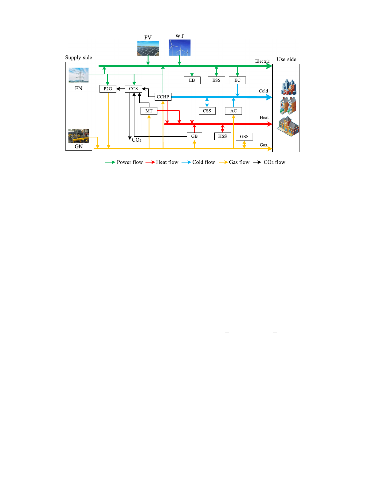
The structure of the RIES constructed in this paper considering the
(2) A multi-objective optimization planning model for the regional
uncertainty of source-load forecasting error is shown in Fig. 1.
integrated energy system, considering the uncertainty of source-load
Associated conversion equipment of the RIES from the source side forecasting, is established.
to the load side via intermediate multi-energy coupling is included
(3) NSGA-III is used to solve the multi-objective function, and
in Fig. 1, where the source side is supplied with electricity and gas
a combination of TOPSIS and fuzzy entropy theory is employed to
from the grid and gas network, and the load side consumes energy for
evaluate the planning outcomes.
electric, cold, heat, and gas users. The P2G device in the intermediate
(4) The impact of considering the uncertainty of source-load fore-
coupling equipment absorbs CO2 provided by CCS and consumes elec-
casting on the optimal operation scheduling results of a regional inte-
tricity to convert it into natural gas, CCS captures CO2 gas produced
grated energy system is discussed.
by CCHP, MT, GB, MT consumes natural gas to produce heat and
The rest of this article is organized as follows. Section 2: Energy
electricity, GB consumes gas to produce heat, EB converts electricity
conversion model of regional integrated energy systems. Section 3:
into heat, AC absorbs heat to make the refrigerant evaporate by heat,
Generation of uncertainty scenarios for source-load forecasting in re-
and then absorbs ambient heat and evaporates it in an evaporator to
gional integrated energy systems. Section 4: Construction of planning
achieve refrigeration effect. EB consumes electric energy to generate
models considering uncertainty in source-load forecasting. Section 5:
cold energy, and CCHP converts natural gas into cold, heat and elec-
Demonstration of optimization methods through case studies, with a
tricity to supply the load demand in the RIES. Multi-energy coupled
discussion and analysis of the results. Section 6: The conclusion section
devices do not fully convert from one energy source to another, there
presents the main conclusions and future work.
is the issue of conversion efficiency, so the conversion efficiency needs
to be considered in the modeling.
2. Regional integrated energy system energy conversion model
2.2. The regional integrated energy systems model
RIES is a complex multi-energy coupling system that integrates
electricity supply equipment, cold equipment, heat equipment, electric
In the RIES model, the conversion process and the input–output
and cold/heat storage devices, as well as renewable energy output
energy balance among multiple forms of energy, such as electric,
devices. It is capable of simultaneously meeting users’ diverse energy
heat, cold, and gas, is a pivotal issue. This balance can typically be
needs. To maximize the benefits of the equipment within RIES, it is
articulated through or more mathematical expressions, encapsulating
necessary to analyze the operating mechanisms of each device in the
the conversion efficiency, input and output quantities, as well as the
system and establish corresponding mathematical models to analyze
interactions among diverse energy forms within the system. Based on
the conversion and flow paths of energy within the system. The char-
the general characteristics of the RIES model, the energy conversion
acteristics of multi-energy integration make the optimization planning
processes and input/output energy balance equations for electric, heat,
objectives more diverse. At both the device level and system level,
cold and gas are presented in Eq. (1).
there are differences in various energy links. Therefor, it is crucial to
𝐿 = 𝐶 𝑃 + 𝑃 𝑁 𝑆 𝑆 (1)
clarify the factors affecting energy utilization efficiency during produc-
tion operations and the mechanisms of related factors. Based on this
where 𝐿 is the load matrix; 𝐶 is the coupling matrix; 𝑃 is the multi-
understanding, propose a RIES structure and model that is suitable for
energy supply matrix; 𝑃 𝑁 𝑆 𝑆 is the charging and discharging electricity
multi-objective optimization planning.
matrix of each energy storage device. The multi-energy supply matrix is shown in Eq. (2).
2.1. Structure of regional integrated energy systems
⎡𝑃 𝐸 (𝑡)⎤ ⎡𝑃 𝐸 𝑁(𝑡) + 𝑃 𝑃 𝑉 (𝑡) + 𝑃 𝑊 𝑇 (𝑡) + 𝑃 𝐶 𝐶 𝐻 𝑃 (𝑡) + 𝑃 𝑀 𝑇 ⎤
⎢ 𝑡𝑜𝑡 ⎥ ⎢ 𝑒 𝑒 𝑒 𝑒 𝑒 ⎥
⎢𝑃 𝐶 (𝑡)⎥ ⎢
𝑃 𝐶 𝐶 𝐻 𝑃 (𝑡) + 𝑃 𝐸 𝐶 (𝑡) + 𝑃 𝐴𝐶 (𝑡) ⎥
The RIES system encompasses a diverse array of energy supply
⎢ 𝑡𝑜𝑡 ⎥ = ⎢ 𝑐 𝑐 𝑐 ⎥ (2)
and conversion equipment, including Photovoltaic (PV), Wind Turbine
⎢𝑃 𝐻(𝑡)
𝑃 𝐶 𝐶 𝐻 𝑃 (𝑡) + 𝑃 𝐸 𝐵(𝑡) + 𝑃 𝐺 𝐵(𝑡) + 𝑃 𝑀 𝑇 𝑡𝑜𝑡 ⎥ ⎢ ℎ ℎ ℎ ℎ ⎥
(WT), Micro gas Turbine (MT), Gas Boiler (GB), Electric Chiller (EC), ⎢ ⎥ ⎢ ⎥
⎣𝑃 𝐺 (𝑡)
𝑃 𝑃 2𝐺(𝑡) + 𝑃 𝐺 𝑁 (𝑡) 𝑡𝑜𝑡 ⎦ ⎣ 𝐺 𝐺 ⎦
Absorption Chiller (AC), Electric Boiler (EB), Carbon Capture System
(CCS), Cogeneration of Cold, Heat and Power (CCHP), Power-to-Gas
𝑃 𝐸 (𝑡), 𝑃 𝐶 (𝑡), 𝑃 𝐻 (𝑡), 𝑃 𝐺 (𝑡) represent the total electric, cold, heat and 𝑡𝑜𝑡 𝑡𝑜𝑡 𝑡𝑜𝑡 𝑡𝑜𝑡
(P2G), and Electricity Storage System (ESS) is also included, Heat
gas energy at time 𝑡 respectively. 𝑃 𝐸 𝑁 (𝑡), 𝑃 𝑃 𝑉 (𝑡), 𝑃 𝑊 𝑇 (𝑡), 𝑃 𝐶 𝐶 𝐻 𝑃 (𝑡) 𝑒 𝑒 𝑒 𝑒 3
Z. Su et al.
Energy 319 (2025) 134861
Fig. 1. Structure of the integrated regional energy system.
denotes the electricity generated by EN, PV, WT and CCHP at the
As can be seen from Fig. 1, the electric energy supply equipment
time 𝑡. 𝑃 𝐶 𝐶 𝐻 𝑃 (𝑡), 𝑃 𝐸 𝐶 (𝑡), 𝑃 𝐴𝐶 (𝑡) denotes the cold energy produced by
includes PV, WT, MT, CCHP, and so forth. The mathematical models 𝑐 𝑐 𝑐
CCHP, EC, and AC at time 𝑡. 𝑃 𝐶 𝐶 𝐻 𝑃 (𝑡), 𝑃 𝐸 𝐵(𝑡), 𝑃 𝐺 𝑁 (𝑡) denotes the heat
for each energy supply equipment are presented in Eqs. (5)–(8). ℎ ℎ ℎ
energy produced by CCHP, EB, and GB at time 𝑡. 𝑃 𝑃 2𝐺(𝑡) represents the
The electricity output of Photovoltaic electricity generation system 𝐺
natural gas produced by P2G at time 𝑡, 𝑃 𝐺 𝑁 (𝑡) for purchased natural gas
is susceptible to external weather changes and exhibits strong random- 𝐺 electricity.
ness. The magnitude of the PV output is related to light intensity and
According to the conversion relationship of each unit within the
temperature, and the PV electricity calculation is shown in Eq. (5).
RIES, substituting Eq. (2) into Eq. (1), the energy conversion of electric,
𝑃 𝑃 𝑉 (𝑡) = 𝜂
heat, cold, and gas and the input–output energy balance relationship 𝑒
𝑃 𝑉 𝐴𝐼 (𝑡) (5)
are written as shown in Eq. (3).
where 𝜂𝑃 𝑉 represents the conversion efficiency of PV electricity gener-
ation, 𝐴 denotes the area of the PV array, and 𝐼(𝑡) signifies the light
⎡𝑃 𝐿(𝑡)
⎡𝑃 𝐸 (𝑡) 𝑡𝑜𝑡
⎤ ⎡𝑃 𝐸 𝑆 𝑆(𝑡)⎤ 𝑒 ⎤ 𝑒 ⎢ ⎢ ⎥ ⎢ ⎥
𝑃 𝐿(𝑡)⎥ density. 𝑃 𝐻 (𝑡) ⎢ ℎ ⎥
⎢ 𝑡𝑜𝑡 ⎥ ⎢𝑃 𝐻 𝑆 𝑆(𝑡) ℎ ⎥
The output electricity of the wind turbine WT is closely related to ⎢ ⎥ = 𝐶 ⎢ ⎥ + ⎢ ⎥ (3) 𝑃 𝐶 (𝑡)
𝑃 𝐶 𝑆 𝑆 (𝑡) ⎢ ⎥
⎢ 𝑡𝑜𝑡 ⎥ ⎢ 𝑐 ⎥
the wind speed, as shown in Eq. (6).
⎣𝑃 𝐿(𝑡)⎦ ⎢ ⎥ ⎢ ⎥ 𝑔
⎣𝑃 𝐺 (𝑡)⎦ ⎣𝑃 𝐺 𝑆 𝑆(𝑡)⎦ 𝑡𝑜𝑡 𝑔
𝑃 𝑊 𝑇 (𝑡) = 𝑃 (𝑡) ⋅ 𝐶 𝑒
𝑃 = 0.5𝜌 ⋅ 𝐴𝑇 ⋅ 𝑉 3(𝑡) ⋅ 𝐶𝑃 (6)
where 𝑃 𝐿(𝑡), 𝑃 𝐿(𝑡), 𝑃 𝐿(𝑡) and 𝑃 𝐿(𝑡) and are the demand for elec- 𝑒 𝑐 ℎ 𝑔
where, 𝐶𝑃 is the electricity coefficient of the wind turbine impeller,
tric, cold, heat and air loads respectively; 𝑃 𝐸 𝑆 𝑆 (𝑡), 𝑃 𝐻 𝑆 𝑆 (𝑡), 𝑃 𝐶 𝑆 𝑆 (𝑡), 𝑒 ℎ 𝑐
taken as 0.593; 𝑃𝑊 𝑇 (𝑡) is the actual wind electricity converted by
𝑃 𝐺 𝑆 𝑆 (𝑡) represents the charging and discharging electricity information 𝑔
the wind turbine; 𝑃 (𝑡) represents the theoretical or available wind
of electric, heat, cold, and energy storage systems. 𝑃 𝐸 (𝑡), 𝑃 𝐻 (𝑡), 𝑃 𝐶 (𝑡), 𝑡𝑜𝑡 𝑡𝑜𝑡 𝑡𝑜𝑡
electricity; 𝐴𝑇 is the area swept by the impeller; and 𝜌 is the air density.
𝑃 𝐺 (𝑡) are the system energy supply within the RIES. The multiple 𝑡𝑜𝑡
The relationship between 𝐶𝑃 and tip speed ratio 𝜆 and pitch angle 𝛽 is
energy conversion coupling matrix is shown in Eq. (4). shown in Eq. (7). ⎡ 𝜃 0 0
𝜗𝜂𝐶 𝐶 𝐻 𝑃 ⋅ 𝐾𝐺 ⎤ ⎧ ( ) ( ) ⎢ 𝑒 ⎥ 𝑐 𝑐 ⎪𝐶 2 5
𝑃 (𝜆, 𝛽 ) = 𝑐1 ⋅
− 𝑐3𝛽 − 𝑐4 ⋅ exp − + 𝑐6 ⋅ 𝜆 ⎢ 𝜂𝐸 𝐵 1
0 (𝜗𝜂𝐶 𝐶 𝐻 𝑃 + 𝜎 𝜂𝐺 𝐵)𝐾𝐺 𝜆1 𝜆1 ℎ ℎ 𝑔 ⎥ ⎨ (7) 𝐶 = ⎢ ⎥ (4) ⎪ 1 = 1 − 0.035
⎢(1 − 𝜃)𝜂𝐸 𝐶 𝜂𝐴𝐶 1
𝜗𝜂𝐶 𝐶 𝐻 𝑃 𝐾𝐺 𝜆
𝜆+0.08𝛽 1+𝛽3 𝑐 ℎ 𝑐 ⎥ ⎩ 1 ⎢ ⎥
⎣ 𝜂𝑃2𝐺 0 0
1 − 𝜗 − 𝜎 𝑔 ⎦
where, 𝑐1 = 0.5176, 𝑐2 = 116, 𝑐3 = 0.4, 𝑐4 = 5, 𝑐5 = 21, 𝑐6 = 0.0068.
where 𝜃 is the proportion of electricity allocated to the electricity-using
The function of MT equipment is to convert natural gas into electric
equipment. 𝜗, 𝜎 are the proportion of natural gas consumed by CCHP
and heat, and then distribute it to the energy consumption end. CCHP
and GB, respectively. 𝜃, 𝜗, 𝜎 ∈ [0, 1]; 𝐾𝐺 is the calorific value of natural
uses natural gas as its primary fuel and converts it into electric, heat,
gas; 𝜂𝐶 𝐶 𝐻 𝑃 , 𝜂𝐶 𝐶 𝐻 𝑃 , 𝜂𝐶 𝐶 𝐻 𝑃 , 𝜂𝐸 𝐵, 𝜂𝐺 𝐵, 𝜂𝐸 𝐶 , 𝜂𝐴𝐶 , 𝜂𝑃 2𝐺 are the CCHP,
and cold energy outputs. The model for its converted electric energy 𝑒 ℎ 𝑐 ℎ 𝑔 𝑐 ℎ 𝑔
EB, GB, EC, AC, and P2G multivariate energy conversion efficiencies,
model can be described by the following Eq. (8). { respectively.
𝑃 𝑀 𝑇 (𝑡) = 𝜂𝑀 𝑇 𝑃 𝑀 𝑇 (𝑡)𝐾 𝑒 𝑔 𝑒 𝑔 𝑔 (8)
𝑃 𝐶 𝐶 𝐻 𝑃 (𝑡) = 𝜂𝐶 𝐶 𝐻 𝑃 ⋅ 𝑃 𝐶 𝐶 𝐻 𝑃 (𝑡) 𝑒 𝑒 𝑔
2.2.1. Modeling of energy supply equipment
Multi-energy supply is primarily provided by various equipment.
where, 𝑃 𝑀 𝑇 (𝑡) is the electric electricity generated by the MT; 𝑃 𝑀 𝑇 (𝑡) 𝑒 ℎ
There is a certain degree of loss during the conversion of one energy
is the heat electricity by the MT; 𝜂𝑀 𝑇 is the electricity generation 𝑔 𝑒
source to another, meaning that conversion from one kind of energy to
efficiency; 𝜂𝑀 𝑇 is the rate of waste heat loss; 𝐾 𝑔 ℎ
𝑔 is the calorific value
another is not 100% efficient. Therefore, conversion efficiency needs to
of natural gas; 𝑃 𝑀 𝑇 (𝑡) represents the gas consumption of the MT. 𝑔
be taken into account in the modeling process. The following describes
(2) Modeling of cold energy supply equipment
the four aspects of electric, cold, heat and gas.
Cold energy is mainly provided by EC, AC and CCHP equipment.
(1) Electricity supply equipment model
EC converts electric energy into cold energy, AC converts heat energy 4
Z. Su et al.
Energy 319 (2025) 134861
into cold energy, and the waste heat discharged from CCHP electricity
2.2.3. Carbon dioxide production and consumption model
generation is used to supply cold energy to users through waste heat
CCS captures CO2 produced by CCHP, MT and GB, and the P2G
recovery and utilization equipment. The model for this process is shown
consumes the CO2 captured by CCS. The equation for CO2 collection in Eq. (9). by CCS is given by Eq. (18). ⎧ 𝐸 𝐶
𝑃 𝐸 𝐶 (𝑡) = 𝜂𝐸 𝐶 𝑃 (𝑡)
𝑄𝐶 𝐶 𝑆 (𝑡) = 𝜂𝐶 𝐶 𝐻 𝑃 𝜃𝐶 𝐶 𝐻 𝑃 𝑃 𝐶 𝐶 𝐻 𝑃 (𝑡) + 𝜂𝑀 𝑇 𝑃 𝑀 𝑇 (𝑡) + 𝜂𝐺 𝐵𝑃 𝐺 𝐵(𝑡) (18) ⎪ 𝑐 𝑒𝑐 𝑒 𝑐 𝑜2 𝑐 𝑜2 𝑐 𝑜2 𝑐 𝑜2 𝑐 𝑜2
⎨𝑃 𝐴𝐶(𝑡) = 𝜂𝐴𝐶𝑃 𝐴𝐶(𝑡) (9) 𝑐
In the above equation, 𝑄𝐶 𝐶 𝑆 (𝑡) denotes the CO ⎪ ℎ𝑐 ℎ 𝑐 𝑜 2 collected by CCS at 2
⎩𝑃 𝐶 𝐶 𝐻 𝑃 (𝑡) = 𝜂𝐶 𝐶 𝐻 𝑃 ⋅ 𝑃 𝐶 𝐶 𝐻 𝑃 (𝑡) 𝑐 𝑐 𝑔
time 𝑡, and 𝜂𝐶 𝐶 𝐻 𝑃 , 𝜂𝑀 𝑇 , 𝜂𝐺 𝐵 are the CO 𝑐 𝑜 2 emission rates of CCHP, MT, 2 𝑐 𝑜2 𝑐 𝑜2
and GB, respectively. The electric electricity consumed by the CCS is
where, 𝑃 𝐸 𝐶 (𝑡), 𝑃 𝐴𝐶 (𝑡), 𝑃 𝐶 𝐶 𝐻 𝑃 (𝑡) are the cold electricity generated by 𝑐 𝑐 𝑐 shown in Eq. (19). 𝐸 𝐶
EC, AC, and CCHP, respectively. 𝑃
(𝑡) is the electricity consumption of 𝑒
EC, 𝑃 𝐴𝐶 (𝑡) is the heat electricity consumed by AC, and 𝑃 𝐶 𝐶 𝐻 𝑃 (𝑡) is the
𝑃 𝐶 𝐶 𝑆 (𝑡) = 𝜃𝐶 𝐶 𝑆 𝑄𝐶 𝐶 𝑆 (𝑡) (19) 𝑒 𝑐 𝑜 𝑐 𝑜 ℎ 𝑔 2 2
natural gas consumed by CCHP. 𝜂𝐸 𝐶 , 𝜂𝐴𝐶 and 𝜂𝐶 𝐶 𝐻 𝑃 are the conversion 𝑒𝑐 ℎ𝑐 𝑐
where, 𝑃 𝐶 𝐶 𝑆 (𝑡) and 𝜃𝐶 𝐶 𝑆 are the electric electricity consumed by the 𝑒 𝑐 𝑜 efficiencies, respectively. 2
CCS and the efficiency of CO2 capture, respectively.
(3) Model of heat energy supply equipment
The P2G consumption 𝐶 𝑂2 model is shown in Eq. (20).
heat energy is mainly supplied by MT, CCHP, GB and EB equipment,
𝐺𝑃 2𝐺 = 𝜃𝑃 2𝐺𝑄𝐶 𝐶 𝑆 (20) 𝑐 𝑜 𝑐 𝑜 𝑐 𝑜
and the model for each piece of equipment is given by Eq. (10). 2 2 2 ⎧
Note that 𝐺𝑃 2𝐺, 𝜃𝑃 2𝐺 denote the P2G output natural gas volume and
𝑃 𝑀 𝑇 (𝑡) 𝑐 𝑜2 𝑐 𝑜2
⎪𝑃 𝑀 𝑇 (𝑡) = 𝑒
(1 − 𝜂𝑀 𝑇 − 𝜂𝑀 𝑇 )
the conversion efficiency of CO 𝑔 𝑒
2 to natural gas, respectively. ⎪ ℎ 𝜂𝑀 𝑇 𝑔 ℎ 𝑔 𝑒
⎪𝑃 𝐶 𝐶 𝐻 𝑃 (𝑡) = 𝜂𝐶 𝐶 𝐻 𝑃 ⋅ 𝑃 𝐶 𝐶 𝐻 𝑃 (𝑡) ⎨ ℎ ℎ 𝑔 (10)
3. Generating uncertainty scenarios for source-load forecasting in
⎪𝑃 𝐺 𝐵(𝑡) = 𝜂𝐺 𝐵𝑃 𝐺 𝐵(𝑡)
regional integrated energy systems ⎪ ℎ 𝑔 ℎ 𝑔 ⎪
⎩𝑃 𝐸 𝐵(𝑡) = 𝜂𝐸 𝐵𝑃 𝐸 𝐵(𝑡) ℎ 𝑒ℎ 𝑒
To ensure the safe and stable operation of regional integrated energy
systems while meeting the demand of all loads within the system
where 𝑃 𝑖 is the heat electricity generated by MT, CCHP, GB, and EB, ℎ 𝑗
and maintaining sufficient reserve capacity, it is necessary to consider 𝜂
is the conversion efficiency of each device, 𝑃 𝑀 𝑇 is the electric 𝑖 𝑒
the uncertainty of source-load forecasting during the planning phase
electricity generated by the MT, 𝑃 𝐸 𝐵 is the electric electricity input 𝑒
of RIES. The forecasting results of wind and photovoltaic electricity
into the EB, and 𝑃 𝐶 𝐶 𝐻 𝑃 (𝑡) and 𝑃 𝐺 𝐵(𝑡) are the natural gas consumption 𝑔 𝑔
generation are influenced by natural conditions and other external fac- of CCHP and GB respectively.
tors, leading to discrepancies between predicted and actual generation;
(4) Natural gas supply equipment model
similarly, there are discrepancies between load forecasting and actual
The P2G consumes electricity to utilize the carbon dioxide collected
demand. When these discrepancies exceed a certain threshold, they
by the CCS and convert it into natural gas when there is an excess of must be taken into account.
electricity within the RIES system. No other added gases are considered
Source-load forecasting uncertainty is a major cause of the volatility
and uncertainty in energy supply and demand, affecting various aspects
in this paper. The model is given by Eq. (11).
of electricity balance and operational scheduling in regional integrated
𝑄𝑃 2𝐺(𝑡) = 𝜂𝑃 2𝐺𝑃 𝑃 2𝐺(𝑡) (11) energy systems. These include: 𝑔 𝑔 𝑒
(1) Difficulty in maintaining supply–demand balance
where, 𝑄𝑃 2𝐺(𝑡) is the P2G gas production electricity, 𝑃 𝑃 2𝐺(𝑡) is the 𝑔 𝑒
The volatility between energy supply and demand makes it difficult
electricity consumption, and 𝜂𝑃 2𝐺 is the conversion efficiency. 𝑔
for the system to maintain a balanced state. (2) Increased operating costs
The uncertainty of source-load forecasting can elevate the operation
2.2.2. Energy storage model and maintenance costs of RIES.
Energy storage model using a unified model as shown in Eqs:
(3) Reduced energy utilization efficiency (12)–(17).
Uncertainty affects the energy utilization efficiency of the system,
potentially leading to energy waste or shortages in cases of supply–
𝛾𝑛𝑐 ℎ(𝑡) + 𝛾𝑛𝑑 𝑖𝑠(𝑡) ≤ 1 (12)
demand imbalance, thereby reducing effective energy utilization.
(4) Challenges in system planning and design
𝑇 𝑛𝑠𝑠 = 𝑇 𝑛𝑠𝑠 (13)
Uncertainty complicates the process of system planning and design. 𝑛𝑒𝑛𝑑 𝑛0
During the design and planning phase of regional integrated energy
systems, it is crucial to consider the interactions between different
𝛾𝑛𝑑 𝑖𝑠(𝑡)𝑃 𝑛𝑠𝑠
≤ 𝑃 𝑛𝑠𝑠 (𝑡) ≤ 𝛾 (14)
energy forms and the impact of uncertainty on system performance.
𝑛𝑑 𝑖𝑠,min
𝑛,𝑑 𝑖𝑠
𝑛𝑑 𝑖𝑠(𝑡)𝑃 𝑛𝑠𝑠
𝑛𝑑 𝑖𝑠,max
3.1. Sampling uncertainty scenarios for source-load forecasting
𝛾𝑛𝑐 ℎ(𝑡)𝑃 𝑛𝑠𝑠
≤ 𝑃 𝑛𝑠𝑠 (𝑡) ≤ 𝛾 (15) 𝑛𝑐 ℎ,min 𝑛,𝑐 ℎ
𝑛𝑐 ℎ(𝑡)𝑃 𝑛𝑠𝑠 𝑛𝑐 ℎ,max
The uncertainty of source-load forecasting errors is influenced by
𝑇 𝑛𝑠𝑠(𝑡 + 1) = 𝑇 𝑛𝑠𝑠(𝑡) + (𝜂𝑛𝑠𝑠 𝑃 𝑛𝑠𝑠(𝑡) − (1∕𝜂𝑛𝑠𝑠 )𝑃 𝑛𝑠𝑠 (𝑡))𝛥𝑡 (16)
various factors, such as wind speed, solar radiation intensity, and load 𝑛 𝑛
𝑛𝑐 ℎ 𝑛𝑐 ℎ
𝑛𝑑 𝑖𝑠
𝑛𝑑 𝑖𝑠
demand. Existing research methods primarily describe the uncertainty
of source-load forecasting errors using probability density functions
𝑇 𝑛𝑠𝑠 ≤ 𝑇 𝑛𝑠𝑠(𝑡) ≤ 𝑇 𝑛𝑠𝑠 (17) 𝑛 min 𝑛 𝑛 max
fitted to specific distributions. However, the probability density dis-
tribution of source-load uncertainties in RIES is asymmetric, making
where 𝛾𝑛𝑐 ℎ(𝑡), 𝛾𝑛𝑑 𝑖𝑠(𝑡) are the charging and discharging flags, 𝑇 𝑛𝑠𝑠(𝑡 + 1) 𝑛
it challenging to accurately represent this uncertainty using specific
and 𝑇 𝑛𝑠𝑠(𝑡) denote the final and starting capacity at times 𝑡 + 1 and 𝑡 𝑛
probability functions. This, in turn, impacts the early-stage planning
respectively; 𝜂𝑛𝑠𝑠 and 𝜂𝑛𝑠𝑠 are the charging and discharging efficiency 𝑛𝑐 ℎ
𝑛𝑑 𝑖𝑠
and capacity allocation of RIES.
of various energy storage devices, and 𝑃 𝑛𝑠𝑠(𝑡) and 𝑃 𝑛𝑠𝑠 (𝑡) represent the
To simulate uncertainty scenarios, this paper employs the Latin 𝑛𝑐 ℎ
𝑛𝑑 𝑖𝑠
charging and discharging electricity of various energy storage devices.
hypercube sampling method, using electric, cold, heat, and gas load 5
Z. Su et al.
Energy 319 (2025) 134861
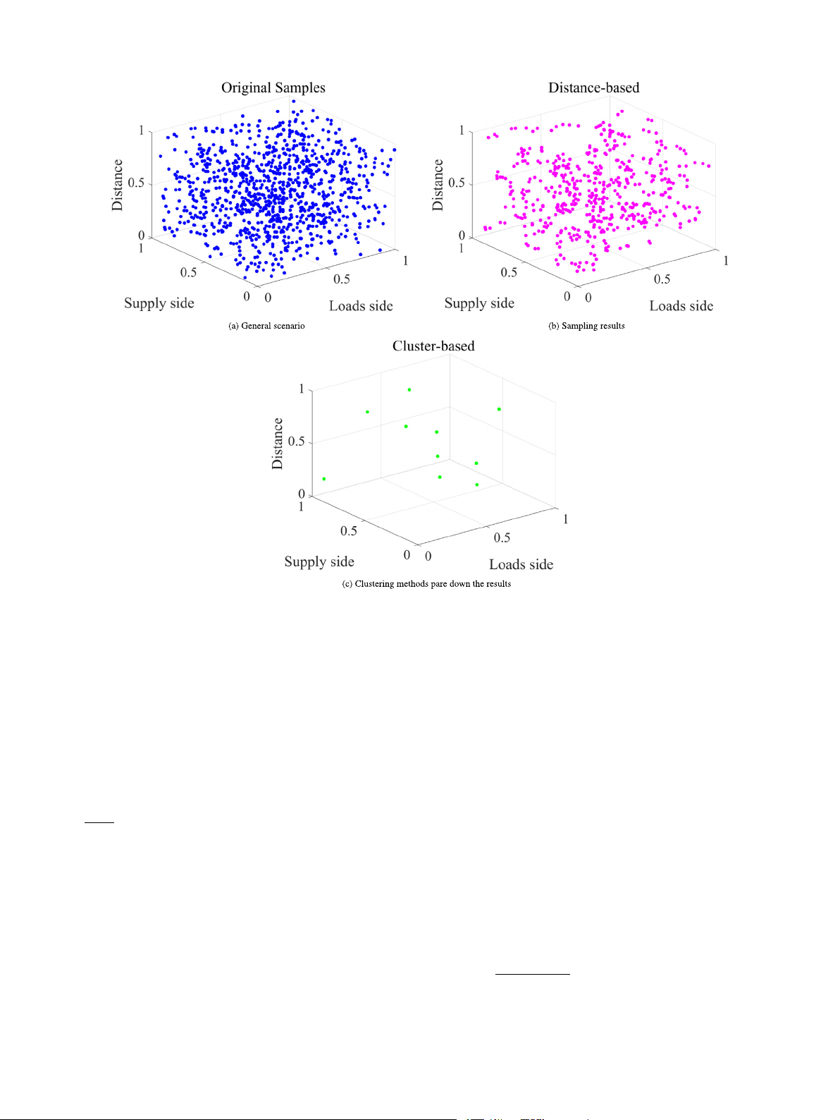
Fig. 2. Uncertainty scenario generation process and reduction results.
demand and forecasting errors as sampling sources. By conducting in the range of [0, 1].
multiple random samples, a large number of potential source-load (3) Perturbation ordering
uncertainty scenarios are generated. The Latin hypercube sampling
To maintain independence between samples, each column in matrix
method ensures that sampling points are selected uniformly, distribut-
𝐴0 is rearranged to obtain the final sampling matrix 𝐴, which represents
ing them as evenly as possible across each row and column, thereby
the uncertainty in source-load forecasting errors, as shown in Fig. 2(a).
enhancing the efficiency and accuracy of sampling process. The specific
implementation steps are as follows:
3.2. Scenario classification and reduction
(1) Define the sampling space and partition the intervals
Assume that the source load forecasting error is an 𝑚-dimensional
To reduce the computational load, cluster and reduce the uncer-
random vector 𝑋 = [𝑋1, 𝑋2, … 𝑋𝑚], where the sampling space for each
tainty scenario set of the original sampling source load forecasting. The
𝑋𝑖 is [𝑐𝑖, 𝑏𝑖]. Divide each dimension 𝑋𝑖 into 𝑁 probability intervals, with
specific implementation steps are as follows:
the width of each interval as shown in Eq. (21). Step 1: Initialization
𝑏𝑖 − 𝑐𝑖 𝛥𝑥
Randomly select 𝐷 scenarios as the initial cluster centers. 𝑖 = (21) 𝑁 Step 2: Reordering
Select 𝐾 scenarios from the total scenario set 𝐴 for reordering,
(2) Generate a random order and select points within intervals
obtaining the sorted matrix 𝐴1. The reordering calculation process is
Randomly select a number from each interval in every dimension
shown in Eq. (23), and the sorting result is shown in Fig. 2(b).
to generate a random permutation of integers from 1 to 𝑁. For each
dimension 𝑖 and the corresponding number 𝑗 in the permutation, cal-
𝐴2 = 𝐴1{(𝐾𝜔 − 𝐾1 ⋅ cos 𝜃 , 𝐾𝜔 + 𝐾1 ⋅ cos 𝜃), 1 ∶ 𝑚} (23)
culate the corresponding point within interval [𝑐𝑖 + (𝑗 − 1)𝛥𝑖, 𝑐𝑖 + 𝑗 𝛥𝑖].
where 𝜔 ∈ [0, 1], 𝐾
Then, obtain the 𝑛th sampling value through inverse transformation.
𝜔 = 𝐾 ⋅ 𝜔, 𝜃 ∈ [0, 90]. Step 3: Distance Calculation
Arrange each of the 𝑁 sampling values from each dimension into a For each scenario 𝑆
single column, resulting in an initial sampling matrix 𝐴
𝑖 in 𝐴1, calculate its distance to all cluster centers 0 of dimensions 𝑠
𝑁 × 𝑚. The expression for element 𝑎
𝑖, as shown in Eq. (24).
𝑚𝑛 within matrix 𝐴0 is given by √ √ Eq. (22). √ 𝑛 ∑ 𝑑(𝑠 √
𝑖, 𝑐𝑗 ) =
(𝑠𝑖𝐷 − 𝑐𝑗 𝐷)2 (24)
𝑎𝑚𝑛 = 𝑌 −1(𝑠 𝑚
𝑚𝑛∕𝑁 + (𝑛 − 1)∕𝑁 ) (22) 𝐷=1
where 𝑌 −1 is the inverse cumulative distribution function of M- 𝑠 𝑚
𝑖𝑘 is the 𝑘th scenario of scenario 𝑠𝑖, and 𝑐𝑗 𝑘 is the cluster center 𝑐𝑗 and
dimensional variables; 𝑠𝑚𝑛 is a uniformly distributed random variable the 𝑘th scenario. 6
Z. Su et al.
Energy 319 (2025) 134861 Step 4: Update and Iterate
4.2.1. Multi-objective optimization model
Recalculate the center of each cluster, as shown in formula Eq. (25).
These objectives often exhibit complex and conflicting relationships, 1 ∑
making it challenging to accurately describe the system’s true situation 𝑐𝑗 = | 𝑠𝑖 (25) | |
with a single objective. Therefore, a multi-objective optimization model
|𝐶𝑗|| 𝑠𝑖∈𝐶𝑗
is established, with system economic performance, environmental im- | | where, 𝐶
pact, and reliability serving as its objectives. The specific model is
𝑗 is the set of all scenarios in cluster 𝑗, ||𝐶𝑗|| is the number of
scenarios in cluster 𝑗. Assign each scenario to the nearest cluster center outlined as follows.
iteratively until the cluster centers no longer change significantly.
⎧min𝐹(𝑋) = min𝑓 Step 5: Scenario Selection ⎪ 𝑖(𝑋)
⎪𝑠𝑢𝑏𝑗 𝑒𝑐 𝑡 ∶ 𝑔(𝑋) ≤ 0,𝑘(𝑋) = 0
Select one representative scenario from each cluster, taking the ⎨ (26)
𝛺 = [𝑃 𝑉 , 𝑊 𝑇 , 𝑀 𝑇 , 𝐶 𝐶 𝑆 , 𝑃 2𝐺 , 𝐸 𝑆 𝑆 , 𝐺 𝑆 𝑆 , 𝐻 𝑆 𝑆 , 𝐺 𝐵 , 𝐶 𝐶 𝐻 𝑃 ]
cluster center as the representative. This obtains the final scenario ⎪ ⎪𝑋 ∈ 𝛺
reduction result, as shown in Fig. 2(c). ⎩
where, 𝑓 (𝑋) represents the objective function, defined as 𝑓
4. Consideration of the construction of a model for source-load 1(𝑋) = 𝐶 , and 𝑓
forecasting uncertainty planning
𝑇 𝑂 𝑇 , 𝑓2(𝑋) = 𝐶𝐶 𝑂2
3(𝑋) = 𝐵𝐸 𝑁 , with detailed calculation
formula provided in Section 3.2. 𝑋 denotes the set of decision vari-
ables, specifically the capacities of the equipment. 𝑔(𝑋) stands for the
This section establishes the basic framework of a model that takes
inequality constraints, 𝑘(𝑋) represents the equality constraints, and 𝛺
into account the uncertainty of source-load forecasting. A multi- is the decision space.
objective optimization function is established with the goals of eco-
nomic, environmental, and reliability. The objective of minimizing
4.2.2. Optimization objective
total cost represents the primary economic goal, minimizing carbon (1) Economic Objective
emissions signifies the environmental goal, and minimizing purchased
The economic objective consists of the initial investment cost, an-
energy embodies the reliability goal. Additionally, the specific solution
nual operation and maintenance cost, and purchased energy cost. Each
process and methods utilized in the model are also provided.
cost is represented by the Eqs. (27)–(31).
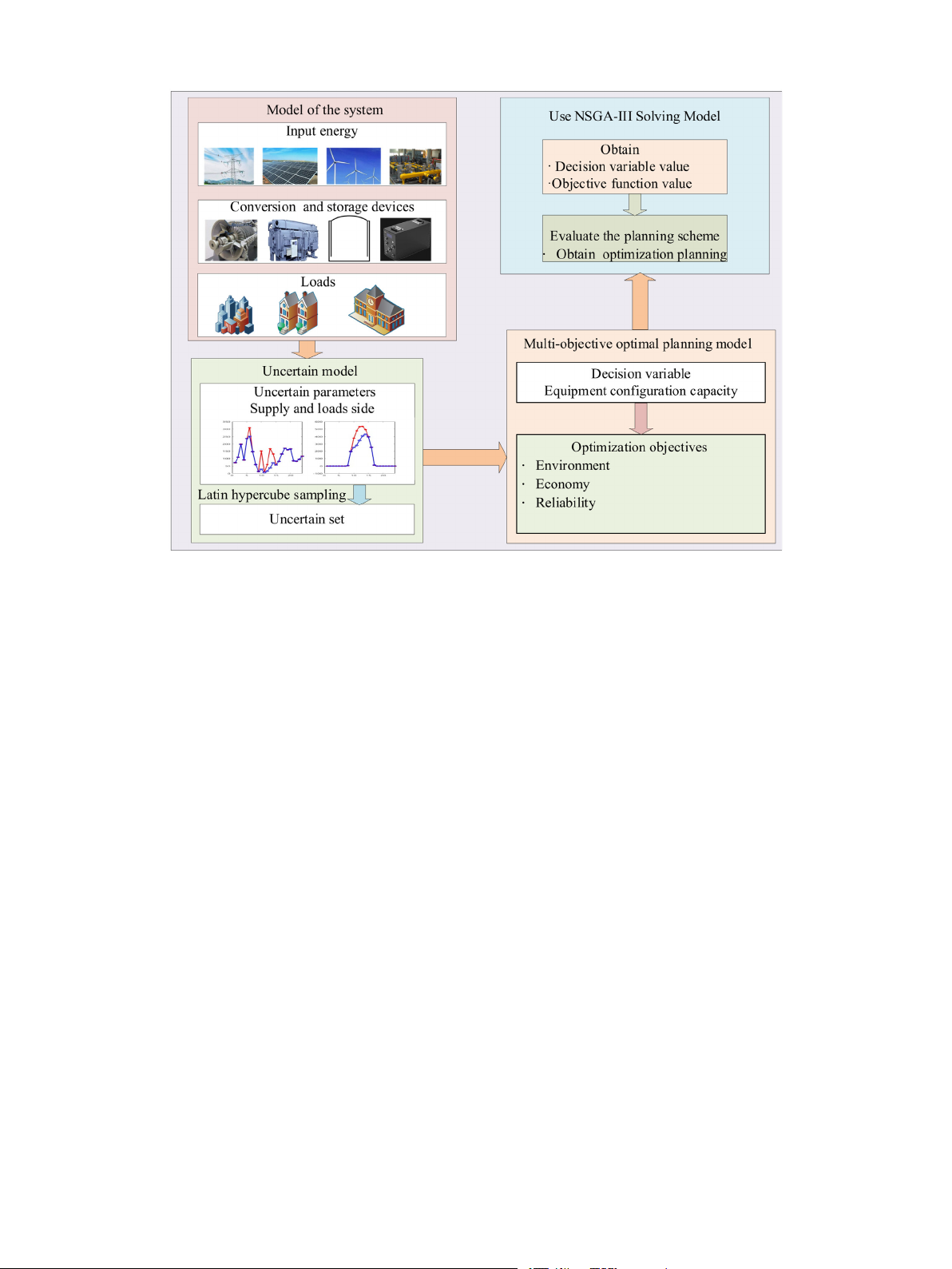
4.1. Multi-objective optimal planning framework
min 𝐶𝑇 𝑂 𝑇 = 𝐶𝐼 𝐼 𝐶 + 𝐶𝑂 𝑀 + 𝐶𝐶 𝑂 𝐸 (27) ∑
According to the characteristics and optimization objectives of RIES,
𝐶𝐼 𝐼 𝐶 =
𝑐𝐼 𝐼 𝐶 ,𝐿 ⋅ 𝐸𝐿 ⋅ 𝜔𝐿 (28)
the basic framework for constructing a multi-objective optimization 𝐿
planning model is illustrated in Fig. 3. First, the established RIES
where 𝑐𝐼 𝐼 𝐶 ,𝐿 is the equivalent annual value coefficient of the planning
system utilizes historical data to predict source load data and cal-
object, calculated as in Eq. (29), 𝐸𝐿 is the capacity of the planning
culate the forecasting error. Based on the obtained forecasting er-
object, and 𝜔𝐿 is the unit capacity investment cost of the corresponding
ror, an uncertainty scenario set is established, categorized, and subse- equipment.
quently reduced. Then, a multi-objective optimization planning model
𝑟(1 + 𝑟)𝑇
is constructed, incorporating total cost, carbon dioxide emissions, and
𝑐𝐼 𝐼 𝐶 ,𝐿 = (29)
(1 + 𝑟)𝑇 − 1
purchased energy as key factors. Finally, the NSGA-III algorithm is
employed to solve the multi-objective optimization function, yielding
𝑟 is the discount rate, which is set to 7% in this paper, and 𝑇 equipment
the Pareto solution set. The final planning results are derived using the
planning period in years. The annual operation and maintenance cost
TOPSIS and fuzzy entropy theory methods. is calculated as Eq. (30).
In the planning framework, firstly, the established RIES system ∑ 365 ∑ 24 ∑
utilizes historical data to predict the source load data and calculate 𝐶𝑂 𝑀 =
𝑐𝑜𝑚𝐸𝑒𝛥𝑡𝛥𝑑 (30) 𝑖 𝑑=1 𝑡=1
the forecasting error. Then, based on the obtained forecasting error, an
uncertainty scenario set is created, classified, and reduced. Secondly,
where 𝑖 denotes the equipment, 𝐶 is the maintenance cost, and 𝐸 cor-
a multi-objective optimal planning model is established, incorporating
responds to the capacity size of the equipment. The cost of purchased total cost, CO
energy is calculated in Eq. (31).
2 emissions, and purchased energy as key objectives.
Finally, NSGA-III is used to solve the multi-objective function, yielding 365 ∑ 24 ∑ 365 ∑ 24 ∑ 𝐶 𝑐 𝑐
the Pareto front as a solution set. TOPSIS and fuzzy entropy methods
𝐶 𝑂 𝐸 =
𝑒𝑃𝑏𝑢𝑦𝛥𝑡𝛥𝑑 +
𝑔 𝐺𝑏𝑢𝑦𝛥𝑡𝛥𝑑 (31) 𝑑=1 𝑡=1 𝑑=1 𝑡=1
are then employed to derive the final decision variable values from this solution set.
where 𝑐𝑒 and 𝑐𝑔 are the time-of-day prices of purchased energy, and
𝑃𝑏𝑢𝑦 and 𝐺𝑏𝑢𝑦 are the amounts of purchased electricity and natural gas,
4.2. Objective function respectively. (2) Environmental Objectives
The problem addressed is how to determine the capacity of equip-
Total CO2 emissions are comprised of carbon emissions from CCS
ment in RIES. Therefore, the decision variables for the multi-objective
within the RIES system and indirect carbon emissions from electricity
optimization model encompass the rated capacities of gas turbines,
purchased off the grid. Smaller values indicate higher environmental
absorption chillers/heaters, the rated cold and heat capacities of air-
targets. Environmental objectives are calculated as in Eq. (32).
source heat pumps, the rated capacity of electric boilers, the capacities
min 𝐶𝑐 𝑜 = 𝑄𝐸 𝑀 + 𝑈 (32) 2 𝑐 𝑜
𝑐 ,𝑒𝑃 𝐸 𝑁 𝑒
of photovoltaic electricity generation, the capacities of wind electric- 2
ity generation, and the installed capacities of various energy storage
where 𝐶𝑐 𝑜 is the total CO is shown 2
2 emissions, The calculation of 𝑄𝐸 𝑀 𝑐 𝑜2
systems. A multi-objective optimization function is established, with
in Eq. (37), 𝑃 𝐸 𝑁 is the purchased electricity consumed, and 𝑈 𝑒
𝑐 ,𝑒 are the
economic performance, environmental impact, and reliability as its CO2 emission factors.
objectives. The economic objective aims to minimize economic invest- (3) Reliability
ment and operation & maintenance; the environmental objective seeks
The lower the total purchased electricity of the RIES, the higher its
to minimize carbon dioxide emissions; and the reliability objective
reliability is. The reliability indicator is calculated as in Eq. (33).
strives to minimum the amount of energy purchased from outside the 𝑃 𝐸 𝑁 𝑃 𝐺 𝑁 𝑒 𝑔 system.
min 𝐵𝐸 𝑁 = ( + )100% (33) 𝑃𝑒 𝑃𝑔 7
Z. Su et al.
Energy 319 (2025) 134861
Fig. 3. RIES planning framework considering source load forecasting error uncertainty.
𝐵𝐸 𝑁 denotes the total amount of purchased energy in the entire RIES,
where 𝑃 𝐸 𝐶 , 𝑃 𝐸 𝐶 represent the minimum and maximum values of EC, min max
and the smaller its value, the higher the reliability of the system.
respectively, while 𝑃 𝐶 𝐶 𝐻 𝑃 and 𝑃 𝐶 𝐶 𝐻 𝑃 represent the minimum and min max
maximum values of CCHP, respectively. 4.3. Constraints (2) CO2 Balance Constraints
𝑃 𝐶 𝐶 𝐻 𝑃 (𝑡) ≤ 𝑃 𝐶 𝐶 𝐻 𝑃 (𝑡 + 1) − 𝑃 𝐶 𝐶 𝐻 𝑃 (𝑡) ≤ 𝑃 𝐶 𝐶 𝐻 𝑃 (𝑡) (36) 𝑔 min 𝑔 𝑔 𝑔 max
In order to ensure that the optimal results comply with the multiple
constraints of the actual planning, further consideration needs to be
𝑄𝐸 𝑀 (𝑡) = 𝑄𝐺 𝐵(𝑡) + 𝑄𝑀 𝑇 (𝑡) + 𝑄𝐶 𝐶 𝐻 𝑃 (𝑡) − 𝑄𝑃 2𝐺(𝑡) − 𝑄𝐶 𝐶 𝑆 (𝑡) (37) 𝑐 𝑜 𝑐 𝑜 𝑐 𝑜 𝑐 𝑜 𝑐 𝑜 𝑐 𝑜
given to the range of values of the optimal variables as well as the 2 2 2 2 2 2
constraint relationships among the variables. The constraints mainly
where, 𝑃 𝐶 𝐶 𝐻 𝑃 (𝑡), 𝑃 𝐶 𝐶 𝐻 𝑃 (𝑡) are the upper and lower limits of natural 𝑔 min 𝑔 max
include two types: equation constraints and inequality constraints.
gas consumed by CCHP; 𝑄𝐺 𝐵(𝑡), 𝑄𝑀 𝑇 (𝑡), and 𝑄𝐶 𝐶 𝐻 𝑃 (𝑡) are CO 𝑐 𝑜 2 emitted 2 𝑐 𝑜2 𝑐 𝑜2
Equation constraints are used to ensure that the supply and demand
by GB, MT, and CCHP respectively; 𝑄𝑃 2𝐺(𝑡) is CO 𝑐 𝑜 2 consumed by P2G; 2
allocations are balanced, while inequality constraints are used to limit
and 𝑄𝐶 𝐶 𝑆 (𝑡) is CO 𝑐 𝑜 2 collected by CCS. 2
the feasible solution space of the optimal planning.
(3)Energy Purchasing Constraints
When internal electricity and natural gas supplies cannot meet the
4.3.1. Electricity balance constraints
load demand, it needs to be purchased from the external grid, subject
The energy balance of electric, cold, heat, and gas is used as a to the following constraints: {
constraint condition for the objective function. Electricity demand is
0 ≤ 𝑃 𝐸 𝑁 (𝑡) ≤ 𝑃 𝑒 𝑏𝑢𝑦,max (38)
met by photovoltaics, wind turbines, gas turbines, grid, and electricity
0 ≤ 𝑃 𝐺 𝑁 (𝑡) ≤ 𝐺 𝐺 𝑏𝑢𝑦,max
storage. The heat load is shared by CCHP, absorption chiller, electric
where 𝑃𝑏𝑢𝑦,max and 𝐺𝑏𝑢𝑦,max denote the maximum amounts of purchased
boiler, and heat storage. Cold loads are met by AC and EC. The energy
electricity and natural gas, respectively.
supply strategy is based on the cold energy requirement to determine
the heat energy need, and the remaining shortfall is supplied by electric
4.4. Solution method energy.
In addition to the energy balance constraints in Eq. (4)–(19) above,
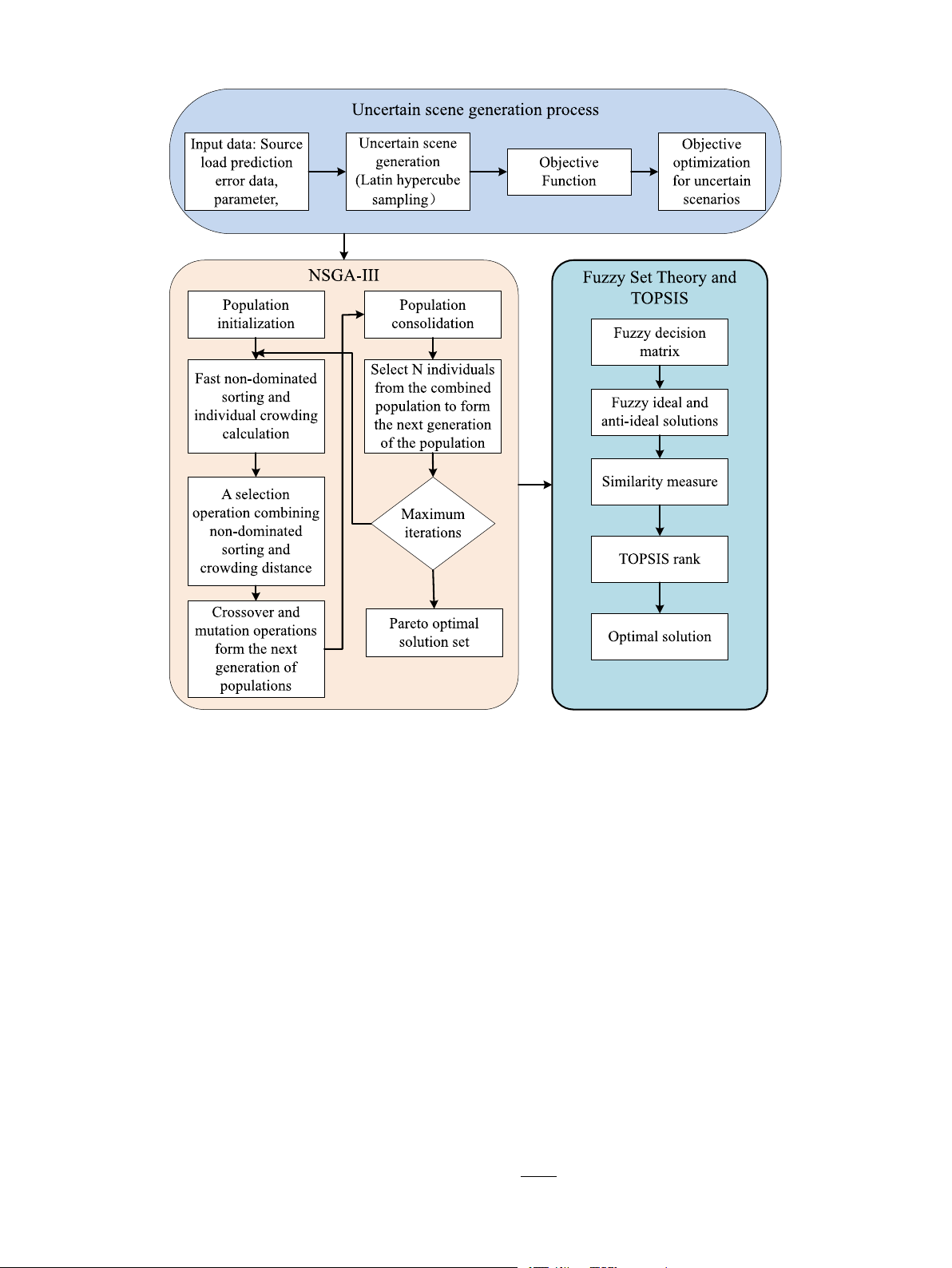
For the proposed multi-objective optimization planning model, this
the output and balance constraints of the following devices should also
paper uses the NSGA-III algorithm for solving. The solution process is
be satisfied. The energy balance constraints, as mentioned above, are
shown in 4 and is implemented in the following two parts: Using NSGA-
supplemented by the following output constraints for each piece of
III to solve the multi-objective optimization model function to obtain equipment.
the three-objective Pareto solution set; Using a combination of fuzzy
(1) Equipment Output Constraints
entropy theory and TOPSIS to obtain the final planning result.
(1) NSGA-III solving multi-objective optimization model process
0 ≤ 𝑃 𝑡 ≤ 𝑃 𝑚 𝑚,max (34)
Step 1: Generate an initial population 𝑃 of size 𝑁.
where 𝑚 ∈ (𝑒, ℎ, 𝑐 , 𝑔), 𝑡 ∈ (𝑃 𝑉 , 𝑊 𝑇 , 𝐸 𝐴, 𝐶 𝐶 𝑆 , 𝐺 𝐵 , 𝑀 𝑇 ). Step 2: Evolution operation
{𝜆𝐸 𝐶𝑃𝐸 𝐶 ≤ 𝑃𝐸 𝐶(𝑡)
Select some individuals from the population for crossover opera- min (35)
𝜆𝐶 𝐶 𝐻 𝑃 𝑃 𝐶 𝐶 𝐻 𝑃 ≤ 𝑃 𝐶 𝐶 𝐻 𝑃 (𝑡) ≤ 𝜆𝐶 𝐶 𝐻 𝑃 𝑃 𝐶 𝐶 𝐻 𝑃
tions to generate a new offspring population 𝑄. New solutions are min max 8
Z. Su et al.
Energy 319 (2025) 134861
Fig. 4. Solution flow of the multi-objective optimal planning model.
produced by exchanging parts of the genetic information between
this paper adopts a method combining fuzzy entropy theory and TOPSIS
parent individuals. Then, apply mutation operations to the offspring
to construct a compromise solution selection strategy. The combination
population to increase its diversity. Merge the parent population 𝑃 and
of these two methods can select the best combined optimal solution
the offspring population 𝑄 to form a new population of size 2𝑁.
from the Pareto optimal solution set. The specific implementation
Step 3: Non-dominated sorting and selection process is as follows:
Perform non-dominated sorting on population 𝑅, dividing the in- Step 1: Initialization
dividuals into multiple non-dominated fronts. NSGA-III introduces a
Assume there is a set composed of 𝑚 decision schemes, each with 𝑛
reference point mechanism to maintain population diversity. First,
attributes, and each attribute is normalized.
generate a set of uniformly distributed reference points in the objective Step 2: Determine Weights
space. Then, associate each individual in the non-dominated fronts with
Determine the weight 𝜔𝑖 for each attribute so that.
the reference points, selecting individuals that are close to the reference 𝑛 ∑
points and are non-dominated to enter the next generation population. 𝜔𝑖 = 1 (39)
Individuals are added to the new population 𝑆 sequentially until its size 𝑖=1 reaches 𝑁.
Step 4: Iteration and termination
(3) Calculation of fuzzy entropy
Repeat the above evolution operations until reaching the preset
For each attribute 𝑖, the fuzzy entropy 𝜇𝑖𝑗(𝑥) is calculated based on
number of iterations or convergence conditions. Then, extract all non-
its fuzzy membership function 𝐻𝑖, as in Eq. (40).
dominated solutions from the final population 𝑆, which constitutes ∞ 𝐻 𝜇
the Pareto optimal solution set for the multi-objective optimization 𝑖 = − ∫
𝑖𝑗 (𝑥) log 𝜇𝑖𝑗 (𝑥)𝑑 𝑥 (40) −∞ problem. (2) Strategy selection
(4) Calculate the weighting coefficients
Multi-objective optimization problems do not have a globally
The weight coefficient 𝐾𝑖 of each attribute is calculated according
unique optimal solution; instead, the solution set consist of a set of
to the fuzzy entropy 𝐻
optimal solutions, known as the Pareto optimal set, which is composed
𝑖, as shown in Eq. (41). 1
of multiple non-dominated solutions. After obtaining the Pareto front, 𝐾𝑖 = (41) 1 + 𝐻𝑖 9
Z. Su et al.
Energy 319 (2025) 134861
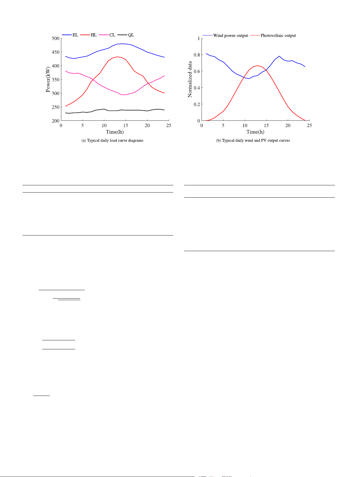
Fig. 5. Typical daily load and scenic output chart. Table 2 Table 3
Parameter settings for energy storage devices. Equipment economic parameters. Items ESS HSS CSS GSS Items Investments O&M costs Rated Life (years) price (CNY/kW) (CNY/kW) electricity (kW) Life (years) 15 20 20 20 Conversion efficiency (%) 0.9 0.85 0.8 0.9 WT 2800 0.03 10/20/30 25
Upper limit of charge and discharge (%) 0.25 0.25 0.85 0.85 PV 2400 0.06 15/10/10 25 Starting value (%) 0.2 0.2 0.2 0.2 MT 3000 0.025 0–800 15 Unit cost (CNY/kW) 600 120 130 100 GB 800 0.04 0–300 15 Energy storage limit (%) 0.8 0.8 0.8 0.8 EC 600 0.03 0–500 15
Lower limit of energy storage (%) 0.2 0.2 0.2 0.2 CCHP 4200 0.02 0–250 15 Capacity (kW) 0–300 0–300 0–300 0-300 CCS 3500 0.02 0–200 15 P2G 6500 0.02 0–300 20 EB 1100 0.01 0–300 15 AC 900 0.02 0–500 20
The larger the fuzzy entropy 𝐻𝑖, the smaller 𝐾𝑖 is, indicating that the
higher the fuzziness of attribute 𝑖 is, the smaller its influence on the decision result.
for a more comprehensive consideration of the fuzziness and uncer-
(5) Calculate the weighted normalization score
tainty among attributes, thereby achieving the best three-objective
For each decision scheme 𝑗, calculate its weighted normalization combined decision scheme.
score 𝜆𝑗 as shown in Eq. (42) √ √ √ 𝑛 ∑ 𝑥
5. Case study 𝑖𝑗 𝜆 √ 𝑗 = √ 𝐴𝑖( √∑ )2 (42) 𝑚 𝑖=1 (𝑥
This paper takes an actual RIES project in Gansu, China, which 𝑗=1 𝑖𝑗 )2
includes electric, cold, and heat systems, as an example. The system
𝑥𝑖𝑗 is the normalized value of scheme 𝑗 on attribute 𝑖.
structure is shown in Fig. 1. Data on actual multi-energy demands and
(6) Calculate the similarity of the schemes
typical wind and solar electricity outputs in 2023 were collected, and
Calculate the distance of each scheme from the positive and nega-
preprocessing was conducted on the collected data prior to planning.
tive optimal solutions as shown in Eq. (43).
To ensure data accuracy and reliability, linear interpolation was used ⎧ √∑
to fill in missing data, while abnormal data were replaced with average ⎪ 2 𝑑+ = 𝑛
(𝑆𝑗 − 𝑆+) ⎨ 𝑗 𝑖=1 𝑖 √
values. The curves of multi-energy electricity demand and wind–solar ∑ (43) ⎪𝑑− = 𝑛 (𝑆 )2
electricity output on a typical day are shown in Fig. 5. There are 365 ⎩ 𝑗 𝑖=1
𝑗 − 𝑆 − 𝑖
days in a year, divided into different seasons, including 182 days in
𝑆+ and 𝑆− are the weighted scores of positive and negative optimal
the transitional season, 94 days in summer, and 89 days in winter. 𝑖 𝑖 solutions on the attribute.
Among the decision variables, include PV, WT, MT, CCS, P2G, ESS,
(7) Calculate the similarity index and rank selection
GSS, HSS, GB, and CCHP. The optimization step size is set to 10 kW.
Calculate the similarity index 𝜁
The overall principle of energy conservation relies on EC and EB as
𝑗 of each scheme, as in Eq. (44). 𝑑−
backups, therefore EC, EB, and CSS are no longer optimized as decision 𝑗 𝜁 variables. 𝑗 = (44) 𝑑+ + 𝑑− 𝑗 𝑗
5.1. Parameter settings for the algorithm
Sort the schemes based on the similarity index and select the scheme
with the highest similarity index as the optimal decision scheme.
This section describes the parameter settings in the case study. The
TOPSIS ranks decision schemes by the calculating the similarity index,
performance parameters of various energy storage devices are set as
utilizing fuzzy entropy to provide a measure of the fuzziness of each
shown in Tables 2 and 3 [14,17], and the price of the purchased energy
attribute. This aids in weight determination and rationality assessment
is shown in Table 4. The relevant parameter settings for NSGA-III are
of decisions. The combination of both fuzzy entropy and TOPSIS allows presented in Table 5. 10
Z. Su et al.
Energy 319 (2025) 134861 Table 4 Table 8 Electric and Gas price. RIES planning results. Items Electric (CNY/kWh) Gas (CNY/m3) Time period Typical PV WT CCS GSS P2G HSS ESS CCHP GB MT Peak 0.9 0.48 8:00–12:00 19:00–21:00 Capacity (kW/kWh) 300 320 200 280 220 220 270 280 250 300 Normal 0.6 0.48 13:00–19:00 21:00–24:00 Low 0.3 0.48 24:00–7:00 in Table 8. Table 5
Parameter settings for NSGA-III.
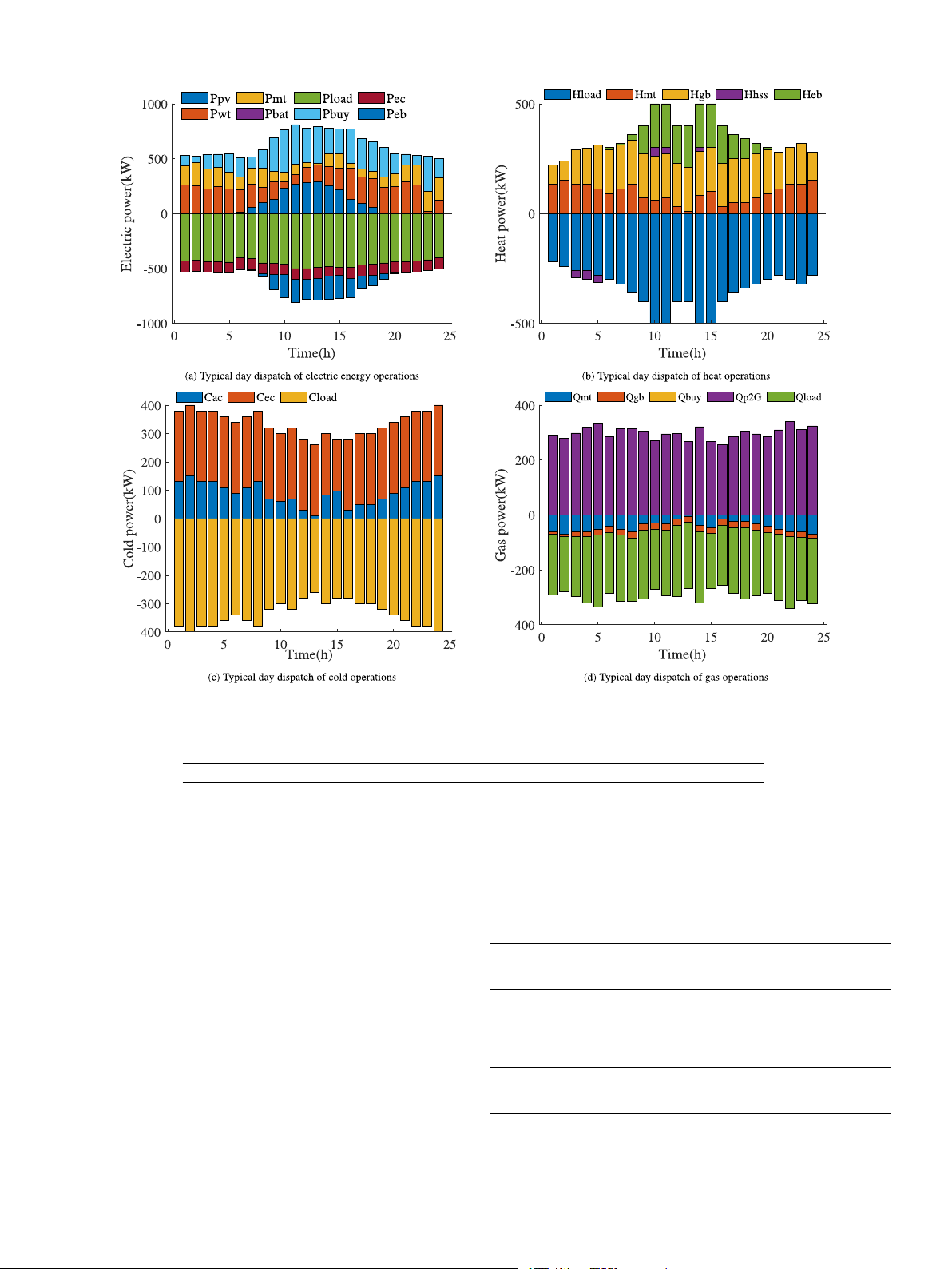
According to the planning results in Table 8, the energy supply Parameters Value
and demand balance operation scheduling results for RIES during the
transition season are shown in Figs. 6, 7, and 8. Population size 300 Crossover probability 0.9
From Fig. 6(a), it can be seen that the RIES prioritizes the use of Mutation probability 0.1
wind electricity to meet the electricity demand. The shortfall is firstly Selection method 5
supplied by MT, and then outsourcing is used to meet the remaining Front levels 6 Number of reference points 100
electricity demand. As time passes, PV starts to generate electricity, Decision variable 12
and the output of MT decreases with the increase in renewable energy Objective function 3
electricity output. For example, at 13:00, the electricity output of MT decreases to a minimum. Table 6
From Fig. 6(b), it can be observed that during the transition season,
Multi-objective optimization collaborative planning results for typical scenarios.
the heat load demand is initially supplied by MT. The shortfall is Typical PV WT CCS GSS P2G HSS ESS CCHP GB MT
provided by GB, and the remaining heat energy is stored in the heat 1 200 330 200 300 300 250 300 300 250 300
storage system. When the heat load demand increases at 10-11:00, the 2 220 310 180 300 280 230 280 270 250 300
heat energy supplied by MT and GB cannot satisfy the system, and at 3 250 300 200 260 300 250 280 300 230 280 4 300 320 200 280 280 220 270 280 250 300
this time, the heat storage system starts to release heat. 5 260 300 160 270 300 240 250 280 240 270
From Fig. 6(c), it is evident that the cold load is primarily supplied 6 200 300 180 200 270 220 200 200 230 250
by AC, and its shortfall is supplemented by EC. 7 250 280 170 250 300 230 260 250 250 300 8 300 320 180 240 300 250 290 280 250 260
Regarding the gas load demand, as shown in Fig. 6(d), it can be 9 320 300 200 250 280 200 250 290 240 290
seen that the gas load demand is mainly satisfied by P2G and purchased 10 300 290 200 300 300 250 300 300 250 300 natural gas.
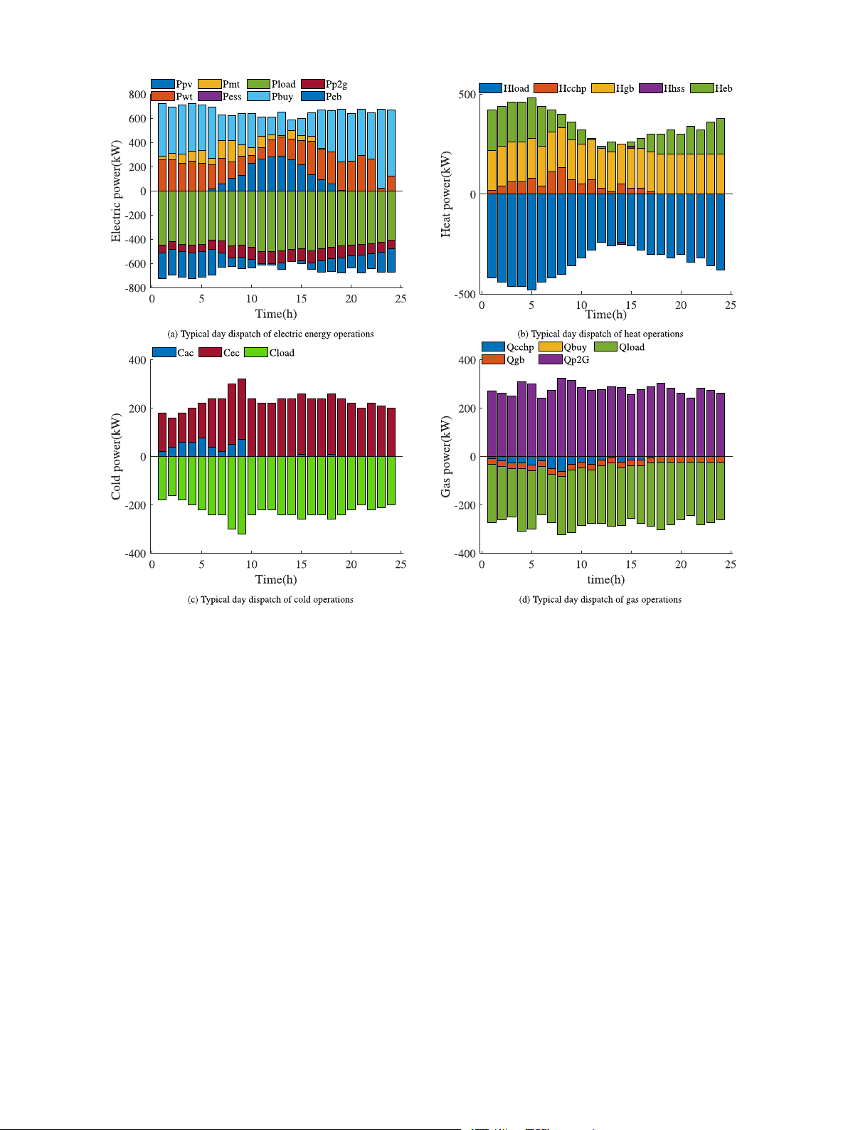
As can be seen from Fig. 7, the demand for heat loads rises during Table 7
the winter months, while the demand for cold loads declines. Concur-
Total cost of RIES system in typical scenarios.
rently, the demand for electricity and natural gas also increases. This Cost price T1 T2 T3 T4 T5 T6 T7 T8 T9 T10
phenomenon can be analyzed as follows; The primary reason for the 𝐶 (Million CNY) 0.34 0.36 0.33 0.3 0.29 0.38 0.35 0.37 0.33 0.3
𝐼 𝐼 𝐶
increased demand is that more electricity and natural gas are typically 𝐶 (Million CNY)
4.12 4.66 4.85 4.39 4.65 4.28 4.67 4.83 4.29 4.71 𝑂 𝑀 𝐶
(Million CNY) 1.13 0.69 1.08 0.75 0.89 0.96 0.85 0.76 0.78 1.05
required to provide heat, thereby meeting the heightened demand for 𝐶 𝑂 𝐸 𝐶
(Million CNY) 5.59 5.71 6.26 5.44 5.83 5.62 5.87 5.96 5.4 6.06
heat loads in winter. Specifically, the rise in electricity demand is 𝑇 𝑂 𝑇
attributed to the fact that heat systems necessitate more electricity to
maintain comfortable indoor temperatures. Additionally, natural gas
demand escalates because many heat systems utilize natural gas to
5.2. Simulation results and analysis generate heat.
The following content mainly discusses case study planning and
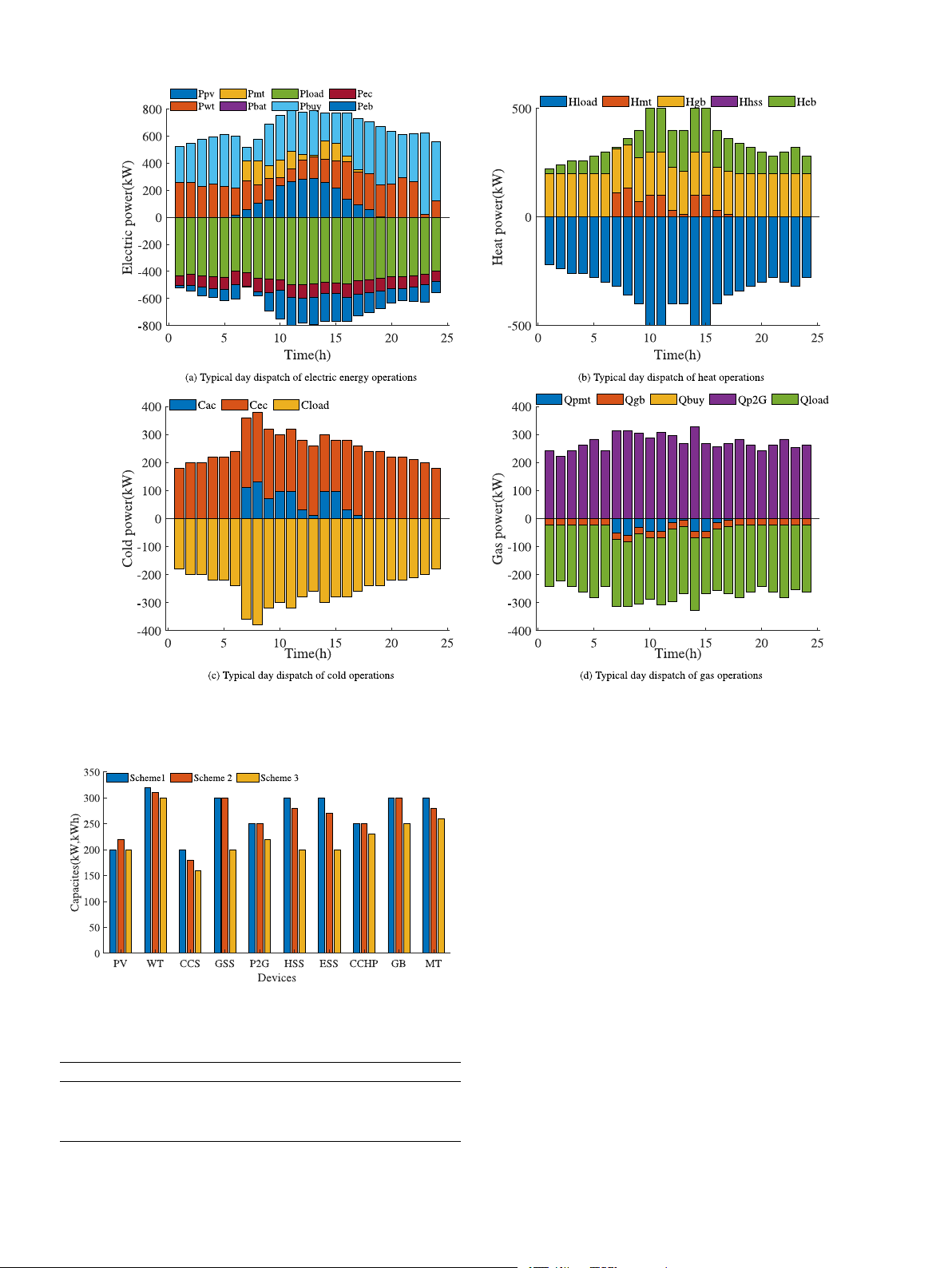
The operational scheduling results for a typical summer day, as
operational results, the impact of uncertainty on planning outcomes,
shown in Fig. 8, indicate that due to the sweltering weather, there is an
and various optimization methods. The results are presented through
increased demand for cold energy. This demand is primarily satisfied
legends and tables respectively, and comparative analyses of different
by Electric Chillers and Cold Storage Systems; any remaining shortfall outcomes are conducted.
is supplemented by EC. Meanwhile, as temperatures rise in summer,
demand for heat energy decreases. In contrast, the demand for natural
5.2.1. Analysis of planning and operation results
gas and electricity increases over the transitional season in summer,
Based on the proposed planning model, which considers uncer-
primarily due to the significant increase in cold energy demand.
tainties in source and load forecasting, the established multi-objective
The regional integrated energy multi-energy supply and demand
function is solved using the NSGA-III method to obtain a Pareto solution
balance is influenced by several factors. On the one hand, operators
set. A strategy combining fuzzy entropy theory and TOPSIS is then
achieve more efficient energy management and load regulation through
employed to select the optimal solution from the Pareto front, yielding
collaboration with the customer side. Operators Provide flexible energy
the final planning result. This strategy aims to achieve optimal planning
supply solutions, while users adjust their load profiles through demand
by balancing the objectives of optimal economics, minimized carbon
response measures. Together. these efforts better cope with fluctuations
dioxide emissions, and high reliability. It primarily considers initial
in the energy market and promote energy supply and demand balance.
investment costs, mid-term fixed maintenance costs, as well as energy
procurement and operational maintenance costs during the operational
On the other hand, user-side multi-type demand response measures phase.
such as users can complement their loads by using different types of
According to the 10 types of typical scenarios described in Sec-
energy. When the demand for electricity is high, natural gas heat can
tion 2.2, the planning results of RIES energy equipment for typical
be increased, thus reducing the demand pressure for electricity. Users
scenarios are listed in Table 6. The components of RIES planning costs
can also time-shift loads by adjusting the timing of energy use. Using are shown in Table 7.
electricity-driven equipment during off-peaks hours and switching to
Based on the planning results in Table 6 and the total system cost
other energy sources during peaks of demand can smooth the load
of typical scenarios in Table 7, the final planning results are presented
curve and avoid supply–demand imbalance. 11
Z. Su et al.
Energy 319 (2025) 134861
Fig. 6. Typical Scenario 8 RIES operational scheduling results. Table 9
The planning results of different schemes are compared. Equipment type Schemes PV WT CCS GSS P2G HSS ESS CCHP GB MT 1 200 320 200 300 250 300 300 250 300 300 Capacity (kW/kWh) 2 220 310 180 300 250 280 270 250 300 280 3 200 300 160 200 220 200 200 230 250 260
5.2.2. Uncertainty impact analysis
In order to verify the validity of the model proposed in this paper, Table 10
simulation analyses of three typical cases are conducted to study the im-
Costing results of different case.
pact of uncertainty on planning capacity. The specific case descriptions Schemes C C C C
𝐼 𝐼 𝐶 𝑂 𝑀 𝐶 𝑂 𝐸 𝑇 𝑂 𝑇 (Million (Million (Million (Million are as follows. CNY) CNY) CNY) CNY)
Case 1: Single objective optimization programming method is ap- 1 0.39 4.96 1.68 7.03
plied without considering the influence of source load forecasting 2 0.36 4.58 1.57 6.51 uncertainty. 3 0.32 4.13 1.12 5.57
Case 2: The single-objective optimization programming method is
applied, considering the impact of source-side forecasting uncertainty.
Case 3: The multi-objective optimization programming method is Table 11
applied, considering the impact of source load forecasting uncertainty.
Output parameters of multi-objective optimization based on different case.
Fig. 9 shows the optimal planning results for different schemes. The Schemes C (Million CNY) C (kg) C (kW) 𝑇 𝑂 𝑇 CO2 CO2
optimization results of three schemes are shown in Table 9, the cost 1 7.03 3256 28%
calculation results of different schemes are shown in Table 10, and 2 6.51 3049 20% 3 5.57 2784 15%
the output parameters of multi-objective optimization are shown in Table 11.
Among the three scenarios, it can be observed that Scenario 3 has
the smallest planning capacity for renewable energy sources and the
CNY less than Scenario 1 and Scenario 2, respectively. Furthermore,
lowest annual total cost, which is 1.46 million CNY and 0.94 million
the lower annual total cost of Case 3 compared to Case 1 and Case 2 12
Z. Su et al.
Energy 319 (2025) 134861
Fig. 7. Typical Scenario 3 RIES operational scheduling results.
indicates that considering the uncertainty in source and load forecast-
and reducing capital expenditure. More flexible and efficient planning
ing errors can further reduce the planning and operational costs of the
strategies can be formulated to enhance resource allocation efficiency
Regional Integrated Energy System. As shown in Table 9, Scenario 3 and return on investment.
also has the smallest carbon dioxide emissions, reduced by 16.9% and (4) Improve system reliability
9.5% compared to Scenario 1 and Scenario 2, respectively, while the
uncertainty planning models that take into account forecasting er-
reliability of the system is improved by 13% and 5%, respectively. The
rors enable the energy system to better cope with sudden changes
reasons for this are mainly the following:
in demand or supply, improving the system’s resilience and reducing
(1) Reducing operational and maintenance costs
the additional costs associated with unexpected events. In conclu-
By considering the source-load forecasting errors more accurately,
sion, by accurately addressing modeling with uncertainty, considering
the required standby capacity of the system can be better assessed.
source-load forecasting errors, the operational efficiency of RIES can
Over-allocation of standby resources to cope with forecasting uncer-
be significantly improved, resource wastage and cost fluctuations can
tainty can be reduced, leading to lower operating costs. Considering
be reduced, and thus cost reductions can be achieved in planning and
the uncertainty of forecasting errors helps to better dispatch avail- operation.
able energy resources, allowing energy production and consumption to
more closely match actual demand, thereby reducing energy waste and
5.2.3. Comparative analysis of different optimization methods associated costs.
To verify the superiority of the optimization method adopted in (2) Reduced uncertainty
this paper, comparisons were made with other heuristic optimization
A Better understanding of and coping with forecasting errors re-
algorithms, including MOEAD, the improved particle swarm optimiza-
duces the volatility of energy market prices due to supply–demand
tion algorithm NMPSO, and NSGA-II. Each algorithm was run 300
imbalances. Stable demand forecasting can mitigate the high costs
times. Table 12 lists the simulation results for the RIES, encompassing
associated with unstable market prices. It can also reduce failures due
planning cost, carbon dioxide emissions, and reliability.
to overloaded systems, ensuring system stability and reliability, and
As can be seen from Table 12, the solution results obtained using
lowering operation maintenance costs.
the NSGA-III algorithm are superior to those of NMPSO, MOEAD, and
(3) Optimizing investment decisions
NSGA-II in terms of overall cost, CO2 emissions, and energy supply
Considering the uncertainty of forecasting errors at the system
reliability. Compared with NSGA-II, the overall cost of the planning
planning stage allows for accurate forecastings of the infrastructure
results is reduced by 0.28 Million CNY, the final CO2 emissions are
investment required, thereby avoiding unnecessary over-investment
decreased by 153 kg, and the reliability is improved by 3%. 13
Z. Su et al.
Energy 319 (2025) 134861
Fig. 8. Typical Scenario 5 RIES operational scheduling results. 6. Conclusion
This study proposes a new planning model for RIES, which in-
tegrates the source-load forecasting error and aims to improve the
system reliability, renewable energy utilization, reduce system invest-
ment and operation maintenance costs, as well as decrease CO2 emis-
sions. Through in-depth theoretical analysis and practical simulation
verification, the following conclusions are drawn:
(1) The planning model proposed in this paper not only comprehen-
sively considers the carrying capacity of various types of equipment in
the RIES, including energy production equipment, energy conversion
equipment, and energy storage equipment, but also incorporates the
planning of carbon capture and storage and power-to-gas equipment.
In addition to conventional investment and operating costs, the model
Fig. 9. Optimal planning results for different scenarios.
pays special attention to system reliability and carbon emissions. The
simulation results significantly demonstrated that in typical scenarios Table 12
9 and 10, the total cost can be reduced by 660,000 CNY when the
Comparison table of results from different optimization algorithms.
installed capacity of renewable energy is increased by 30 kW, which Algorithm C (Million CNY) C (kg) B (kW) 𝑇 𝑂 𝑇 CO2 𝐸 𝑁
verifies the effectiveness of the model in improving energy efficiency NMPSO 7.83 3349 27% and cost control. MOEAD 6.68 3165 22%
(2) By comparing the three different planning scenarios, it is found NSGA-II 5.85 2937 18% NSGA-III 5.57 2784 15%
that the total annual cost of Case 3 is significantly lower than that
of Cases 1 and Cases 2, with reductions of 1.46 million CNY and
0.94 million CNY, respectively. This result provides strong evidence
that an approach that takes into account source-load forecasting error 14
Z. Su et al.
Energy 319 (2025) 134861
uncertainty can further optimize the planning and operating costs of References
the RIES and contribute to the reduction of carbon dioxide emissions,
thereby improving the overall reliability of the system. This finding
[1] Ding T, Hu Y, Bie Z. Multi-stage stochastic programming with nonanticipativity
has important implications for improving the practicality of integrated
constraints for expansion of combined power and natural gas systems. IEEE Trans Power Syst 2018;33:317–28.
planning and operation options for RIES.
[2] Liu Z, Cui Y, Wang J, Yue C, Agbodjan YS, Yang Y. Multi-objective
(3) To promote the development of regional integrated energy sys-
optimization of multi-energy complementary integrated energy systems consid-
tems, concerted efforts from policy guidance by functional departments
ering load prediction and renewable energy production uncertainties. Energy
and technical research are required. The planning model constructed 2022;254:124399.
[3] Wu Z, Li A, Sun Q, Zheng S, Zhao J, Liu P, Gu W. Multistage reliability-
in this paper is applicable to energy planning, policy formulation,
constrained stochastic planning of diamond distribution network: An ap-
infrastructure construction, market operation, and CO2 emissions man-
proximate dynamic programming approach. Int J Electr Power Energy Syst
agement, aiding in energy efficiency improvement, energy optimiza- 2024;156:109701.
tion, and low-carbon transformation. However, it faces challenges such
[4] Hemmati R. Dynamic expansion planning in active distribution grid integrated
with seasonally transferred battery swapping station and solar energy. Energy
as forecasting accuracy, data processing, computational complexity, 2023;277:127719.
system scale, and policy and technological constraints. To overcome
[5] Cui J, Liao C, Ji L, Xie Y, Yu Y, Yin J. A short-term hybrid energy system robust
these challenges and promote the sustainable development of regional
optimization model for regional electric-power capacity development planning
integrated energy systems, it is recommended to strengthen cross-
under different pollutant control pressures. Sustain 2021;13:11341.
departmental collaboration, optimize data sharing, enhance forecasting
[6] Chen Y, Basciftci B, M.Thomas V. Chance-constrained multi-stage stochastic
energy system expansion planning with demand satisfaction flexibility. Int J
technologies, simplify calculations and improve model adaptability.
Electr Power Energy Syst 2024;155:109499.
Additionally, formulate a flexible policy framework, and strengthen
[7] Ji L, Zhang B, Huang G, Cai Y, Yin J. Robust regional low-carbon electricity
public education and participation are also crucial.
system planning with energy-water nexus under uncertainties and complex policy
(4) The current scheme does not consider the conversion relation-
guidelines. J Clean Prod 2020;252:119800.
[8] Wang Q, Luo X, Ma H, Gong N. Multi-stage stochastic wind-thermal generation
ships between hydrogen production, hydrogen storage systems, energy
expansion planning with probabilistic reliability criteria. IET Gener Transm
storage plant systems of RIES. Future studies should incorporate the Distrib 2021;16:517–34.
integration of hydrogen production and storage systems, as well as
[9] Ji L, Zhang B, Huang G, Wang P. A novel multi-stage fuzzy stochastic
system operations, into the planning objectives. This approach aims to
programming for electricity system structure optimization and planning with
energy-water nexus - A case study of Tianjin, China. Energy 2020;190:116418.
achieve a more efficient use of energy and to enhance the reliability and
[10] Domínguez R, Carrión M, Conejo A. Influence of the number of decision stages
robustness of RIES systems. Through continuous improvement of the
on multi-stage renewable generation expansion models. Int J Electr Power Energy
planning model, anticipate that the regional integrated energy system Syst 2021;126:106588.
will become more intelligent, efficient, and environmentally friendly.
[11] Wang B, Wang X, Wei F, Shao C, Zhou J, Lin J. Multi-stage stochastic planning
for a long-term low-carbon transition of island power system considering carbon
price uncertainty and offshore wind power. Energy 2023;282:128349.
CRediT authorship contribution statement
[12] Zeng Q, Zhang B, Fang J, Chen Z. A bi-level programming for multistage co-
expansion planning of the integrated gas and electricity system. Appl Energy 2017;200:192–203.
Zhonge Su: Writing – original draft, Supervision, Resources, Method-
[13] Khaligh V, Anvari-Moghaddam A. Stochastic expansion planning of gas and
ology, Formal analysis. Guoqiang Zheng: Writing – review & editing,
electricity networks: A decentralized-based approach. Energy 2019;186:115889.
Project administration, Conceptualization. Guodong Wang: Supervi-
[14] Li P, Wang Z, Liu H, Wang J, Guo T, Yin Y. Bi-level optimal configuration
sion, Software, Formal analysis. Yu Mu: Writing – review & editing,
strategy of community integrated energy system with coordinated planning and
operation. Energy 2021;236:121539.
Visualization, Investigation. Jiangtao Fu: Visualization, Methodology,
[15] Pan G, Gu W, Lu Y, Qiu H, Lu S, Yao S. Optimal planning for electricity-hydrogen
Data curation. Peipei Li: Writing – review & editing, Visualization,
integrated energy system considering power to hydrogen and heat and seasonal Data curation.
storage. IEEE Trans Sustain Energy 2020;11:2662–76.
[16] Li J, Xu Z, Liu H, Wang C, Wang L, Gu C. A wasserstein distributionally robust
planning model for renewable sources and energy storage systems under multiple
Declaration of competing interest
uncertainties. IEEE Trans Sustain Energy 2023;14:1346–56.
[17] Li J, Yang S, Zhou X, Li J. Multi-objective optimization of regional integrated
energy system matrix modeling considering exergy analysis and user satisfaction.
The authors declare the following financial interests/personal rela-
Int J Electr Power Energy Syst 2024;156:109765.
tionships which may be considered as potential competing interests:
[18] Yang B, Ge S, Liu H, Zhang X, Xu Z, Wang S, Huang X. Regional integrated
This work was supported by the Key project of Henan Province Sci-
energy system reliability and low carbon joint planning considering multiple
ence and Technology Research and Development Program Joint Fund
uncertainties. Sustain Energy Grids Netw 2023;35:101123.
(235200810040, 231111221500), the National Natural Science Foun-
[19] Mu Y, Chen W, Yu X, Jia H, Hou K, Wang C, Meng X. A double-layer planning
method for integrated community energy systems with varying energy conversion
dation of China (62072158), and Science and Technology Project of
efficiencies. Appl Energy 2020;279:115700. Henan Province (242102210197).
[20] Li J, Xu W, Cui P, Qiao B, Feng X, Xue H, Wang X, Xiao L. Optimization
configuration of regional integrated energy system based on standard module. Energy Build 2020;229:110485. Acknowledgments
[21] Guo J, Wu D, Wang Y, Wang L, Guo H. Co-optimization method research
and comprehensive benefits analysis of regional integrated energy system. Appl
This work was supported by the Key project of Henan Province Energy 2023;340:121034.
[22] Lei Y, Wang D, Cheng H, Jia H, Li Y, Ding S, Guo X. A three-layer planning
Science and Technology Research and Development Program Joint
framework for regional integrated energy systems based on the quasi-quantum
Fund, China (235200810040, 231111221500), the National Natural
theory. Int J Electr Power Energy Syst 2024;155:109523.
Science Foundation of China (62072158), and Science and Technology
[23] Oskouei MZ, Abapour M. Strategic operation of a virtual energy hub with the
Project of Henan Province, China (242102210197).
provision of advanced ancillary services in industrial parks. IEEE Trans Sustain Energy 2021;12:2062–73.
[24] Zhang H, Cao Q, Gao H, Wang P, Zhang W, Yousefi N. Optimum design of a
Data availability
multi-form energy hub by applying particle swarm optimization. J Clean Prod 2020;260:121079.
[25] Lin X, Huang G, Zhou X, Zhai Y. An inexact fractional multi-stage programming
Data will be made available on request.
(IFMSP) method for planning renewable electric power system. Renew Sustain Energy Rev 2023;187:113611. 15
Z. Su et al.
Energy 319 (2025) 134861
[26] Sun Q, Wu Z, Gu W, Liu P, Wang J, Lu Y, Zheng S, Zhao J. Multi-stage co-
[28] Liang H, Xu L, Zhao Y, Zhang S, Chen C, Tang J, Yang L, Lin Z. Day-ahead
planning model for power distribution system and hydrogen energy system under
joint scheduling of multiple park-level integrated energy systems considering
uncertainties. J Mod Power Syst Clean Energy 2023;11:80–93.
coupling uncertainty of electricity-carbon-gas prices. Int J Electr Power Energy
[27] Ma Y, Han X, Zhang T, Li A, Song Z, Li T, Wang Y. Research on station-network Syst 2024;158:109933.
planning of electricity- thermal -cooling regional integrated energy system
[29] Cao Y, Wei W, Wang J, Mei S, Shafie-khah M, Catalao JPS. Capacity planning
considering multiple-load clusters and network costs. Energy 2024;131281.
of energy hub in multi-carrier energy networks: A data-driven robust stochastic
programming approach. IEEE Trans Sustain Energy 2020;11:3–14.
[30] Li W, Qian T, Zhang Y, Shen Y, Wu C, Tang W. Distributionally robust chance-
constrained planning for regional integrated electricity–heat systems with data
centers considering wind power uncertainty. Appl Energy 2023;336:120787. 16
Document Outline
- Multi-objective optimal planning study of integrated regional energy system considering source-load forecasting uncertainty
- Introduction
- Regional Integrated Energy System Energy Conversion Model
- Structure of Regional Integrated Energy Systems
- The Regional Integrated Energy Systems Model
- Modeling of Energy Supply Equipment
- Energy Storage Model
- Carbon Dioxide Production and Consumption Model
- Generating Uncertainty Scenarios for Source-Load Forecasting in Regional Integrated Energy Systems
- Sampling Uncertainty Scenarios for Source-Load Forecasting
- Scenario Classification and Reduction
- Consideration of the Construction of a Model for Source-Load Forecasting Uncertainty Planning
- Multi-Objective Optimal Planning Framework
- Objective Function
- Multi-Objective Optimization Model
- Optimization Objective
- Constraints
- Electricity Balance Constraints
- Solution Method
- Case Study
- Parameter settings for the algorithm
- Simulation results and analysis
- Analysis of planning and operation results
- Uncertainty Impact Analysis
- Comparative Analysis of Different Optimization Methods
- Conclusion
- CRediT authorship contribution statement
- Declaration of competing interest
- Acknowledgments
- Data availability
- References
Tài liệu liên quan:
-

Test 1 Academic Set - Climate Change Threats to the Great Barrier Reef
15 8 -

Bìa tiếng anh - Bìa tiếng anh UEH
14 7 -

Đề thi tham khảo môn Tiếng Anh 2023 - Sửa đáp án và câu hỏi_test
20 10 -

Module 3, 4, 5 - Tieng Anh: Reducing Relative Clauses & Tenses
16 8 -

Gợi ý đề thi thử TNTHPT năm 2026 môn tiếng anh
28 14