Textbook English Chapter 13. The costs of Production
Textbook English Chapter 13. The costs of Production.Tài liệu tổng hợp được sưu tầm. Mời mọi người tham khảo
Chủ đề: Tài liệu chung Tiếng Anh 12 528 tài liệu
Môn: Tiếng Anh 12 1.3 K tài liệu
Tác giả:


Preview text:
T CHAPTER
he economy includes thousands of firms that produce the goods
and services you enjoy every day: General Motors produces
automobiles, General Electric produces lightbulbs, and General 13
Mills produces breakfast cereals. Some firms, such as these three, are
large; they employ thousands of workers and have thousands of
stockholders who share the firms’ profits. Other firms, such as the
local general store, barbershop, or café, are small; they employ only
a few workers and are owned by a single person or family. The Costs
In previous chapters, we used the supply curve to summarize
firms’ production decisions. According to the law of supply, firms
are willing to produce and sell a greater quantity of a good when the of Production
price of the good is higher. This response leads to an upward-sloping
supply curve. For many questions, the law of supply is all you need to know about firm behavior.
In this chapter and the ones that follow, we examine firm behavior
in more detail. This topic will give you a better understanding of
the decisions behind the supply curve. It will also introduce you to
a part of economics called industrial organization—the study of how
firms’ decisions about prices and quantities depend on the market
conditions they face. The town in which you live, for instance,
may have several pizzerias but only one cable television company. M O .C K C TO S R TTE U H Y/S D U R E G R EO ; G K C TO S LO /LO M .CO K C O IST 244
PART V FIRM BEHAVIOR AND THE ORGANIZATION OF INDUSTRY
This raises a key question: How does the number of firms affect the prices in a mar-
ket and the efficiency of the market outcome? The field of industrial organization
addresses exactly this question.
Before turning to these issues, we need to discuss the costs of production. All
firms, from Delta Air Lines to your local deli, incur costs while making the goods
and services that they sell. As we will see in the coming chapters, a firm’s costs
are a key determinant of its production and pricing decisions. In this chapter, we
define some of the variables that economists use to measure a firm’s costs, and we
consider the relationships among these variables.
A word of warning: This topic is dry and technical. To be honest, one might even
call it boring. But this material provides the foundation for the fascinating topics that follow. 13-1 What Are Costs?
We begin our discussion of costs at Chloe’s Cookie Factory. Chloe, the owner of
the firm, buys flour, sugar, chocolate chips, and other cookie ingredients. She also
buys the mixers and ovens and hires workers to run this equipment. She then sells
the cookies to consumers. By examining some of the issues that Chloe faces in her
business, we can learn some lessons about costs that apply to all firms.
13-1a Total Revenue, Total Cost, and Profit
To understand the decisions a firm makes, we must understand what it is trying
to do. Chloe may have started her firm because of an altruistic desire to provide
the world with cookies or simply out of love for the cookie business, but it is more
likely that she started the business to make money. Economists normally assume
that the goal of a firm is to maximize profit, and they find that this assumption works well in most cases.
What is a firm’s profit? The amount that the firm receives for the sale of its total revenue
output (cookies) is called total revenue. The amount that the firm pays to buy the amount a firm
inputs (flour, sugar, workers, ovens, and so forth) is called total cost. As the busi- receives for the sale of its
ness owner, Chloe gets to keep any revenue above her costs. That is, a firm’s profit output
equals its total revenue minus its total cost: total cost
Profit 5 Total revenue 2 Total cost the market value of the inputs a firm uses in
Chloe’s objective is to make her firm’s profit as large as possible. production
To see how a firm maximizes profit, we must consider fully how to measure its profit
total revenue and its total cost. Total revenue is the easy part: It equals the quantity total revenue minus total
of output the firm produces multiplied by the price at which it sells its output. cost
If Chloe produces 10,000 cookies and sells them at $2 a cookie, her total revenue is
$20,000. The measurement of a firm’s total cost, however, is more subtle.
13-1b Costs as Opportunity Costs
When measuring costs at Chloe’s Cookie Factory or any other firm, it is important
to keep in mind one of the Ten Principles of Economics from Chapter 1: The cost of
something is what you give up to get it. Recall that the opportunity cost of an item
refers to all the things that must be forgone to acquire that item. When economists
speak of a firm’s cost of production, they include all the opportunity costs of mak-
ing its output of goods and services.
CHAPTER 13 THE COSTS OF PRODUCTION 245
While some of a firm’s opportunity costs of production are obvious, others are less
so. When Chloe pays $1,000 for flour, that $1,000 is an opportunity cost because Chloe
can no longer use that $1,000 to buy something else. Similarly, when Chloe hires work-
ers to make the cookies, the wages she pays are part of the firm’s costs. Because these
opportunity costs require the firm to pay out some money, they are called explicit costs. explicit costs
By contrast, some of a firm’s opportunity costs, called implicit costs, do not require input costs that require
a cash outlay. Imagine that Chloe is skilled with computers and could earn $100 per an outlay of money by
hour working as a programmer. For every hour that Chloe works at her cookie factory, the firm
she gives up $100 in income, and this forgone income is also part of her costs. The total
cost of Chloe’s business is the sum of her explicit and implicit costs. implicit costs
The distinction between explicit and implicit costs highlights a difference input costs that do not
between how economists and accountants analyze a business. Economists are inter- require an outlay of
ested in studying how firms make production and pricing decisions. Because these money by the firm
decisions are based on both explicit and implicit costs, economists include both
when measuring a firm’s costs. By contrast, accountants have the job of keeping
track of the money that flows into and out of firms. As a result, they measure the
explicit costs but usually ignore the implicit costs.
The difference between the methods of economists and accountants is easy to
see in the case of Chloe’s Cookie Factory. When Chloe gives up the opportunity
to earn money as a computer programmer, her accountant will not count this as a
cost of her cookie business. Because no money flows out of the business to pay for
this cost, it never shows up on the accountant’s financial statements. An economist,
however, will count the forgone income as a cost because it will affect the decisions
that Chloe makes in her cookie business. For example, if Chloe’s wage as a com-
puter programmer rises from $100 to $500 per hour, she might decide that running
her cookie business is too costly. She might choose to shut down the factory so she
can take a job as a programmer.
13-1c The Cost of Capital as an Opportunity Cost
An implicit cost of almost every business is the opportunity cost of the financial
capital that has been invested in the business. Suppose, for instance, that Chloe
used $300,000 of her savings to buy the cookie factory from its previous owner.
If Chloe had instead left this money in a savings account that pays an interest rate
of 5 percent, she would have earned $15,000 per year. To own her cookie factory,
therefore, Chloe has given up $15,000 a year in interest income. This forgone $15,000
is one of the implicit opportunity costs of Chloe’s business.
As we have noted, economists and accountants treat costs differently, and this
is especially true in their treatment of the cost of capital. An economist views the
$15,000 in interest income that Chloe gives up every year as an implicit cost of her
business. Chloe’s accountant, however, will not show this $15,000 as a cost because
no money flows out of the business to pay for it.
To further explore the difference between the methods of economists and
accountants, let’s change the example slightly. Suppose now that Chloe did not
have the entire $300,000 to buy the factory but, instead, used $100,000 of her own
savings and borrowed $200,000 from a bank at an interest rate of 5 percent. Chloe’s
accountant, who only measures explicit costs, will now count the $10,000 interest
paid on the bank loan every year as a cost because this amount of money now
flows out of the firm. By contrast, according to an economist, the opportunity cost
of owning the business is still $15,000. The opportunity cost equals the interest on
the bank loan (an explicit cost of $10,000) plus the forgone interest on savings (an implicit cost of $5,000). 246
PART V FIRM BEHAVIOR AND THE ORGANIZATION OF INDUSTRY
13-1d Economic Profit versus Accounting Profit
Now let’s return to the firm’s objective: profit. Because economists and accoun-
tants measure costs differently, they also measure profit differently. An economist economic profit
measures a firm’s economic profit as its total revenue minus all its opportunity costs total revenue minus total
(explicit and implicit) of producing the goods and services sold. An accountant mea- cost, including both
sures the firm’s accounting profit as its total revenue minus only its explicit costs. explicit and implicit costs
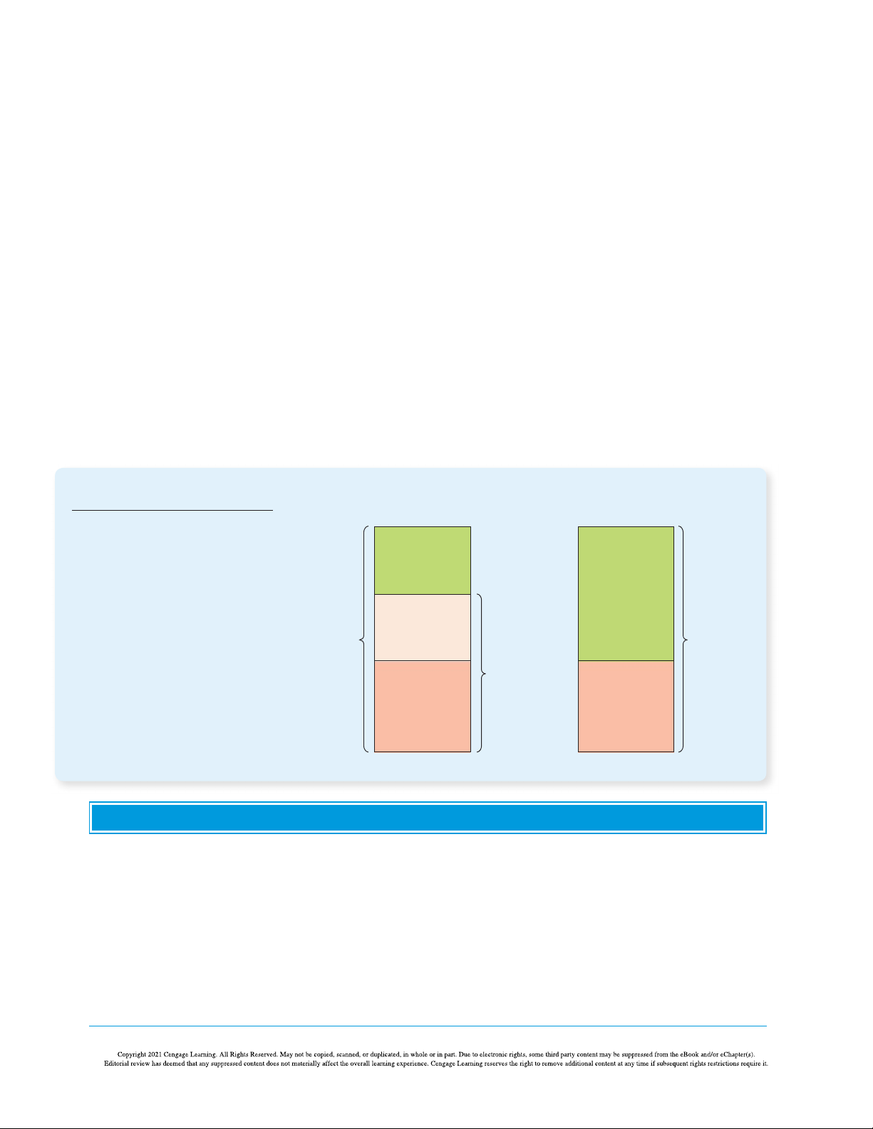
Figure 1 summarizes this difference. Notice that because the accountant ignores
the implicit costs, accounting profit is usually larger than economic profit. For a accounting profit
business to be profitable from an economist’s standpoint, total revenue must exceed total revenue minus total
all the opportunity costs, both explicit and implicit. explicit cost
Economic profit is an important concept because it motivates the firms that
supply goods and services. As we will see, a firm making positive economic profit
will stay in business. It is covering all its opportunity costs and has some revenue
left to reward the firm’s owners. When a firm is making economic losses (that
is, when economic profits are negative), the business owners are failing to earn
enough revenue to cover all the costs of production. Unless conditions change,
the firm owners will eventually close down the business and exit the industry.
To understand business decisions, we need to keep an eye on economic profit. FIGURE 1 How an Economist How an Accountant Views a Firm Views a Firm Economists versus Accountants
Economists include all opportunity
costs when analyzing a firm, whereas Economic
accountants measure only explicit profit
costs. Therefore, economic profit is Accounting
smaller than accounting profit. profit Implicit Revenue costs Revenue Total opportunity costs Explicit Explicit costs costs QuickQuiz
1. Farmer McDonald gives banjo lessons for $20 per
2. Xavier opens up a lemonade stand for two hours.
hour. One day, he spends 10 hours planting $100
He spends $10 for ingredients and sells $60 worth
worth of seeds on his farm. What total cost has he
of lemonade. In the same two hours, he could have incurred?
mowed his neighbor’s lawn for $40. Xavier earns a. $100
an accounting profit of _________ and an economic b. $200 profit of _________. c. $300 a. $50; $10 d. $400 b. $90; $50 c. $10; $50 d. $50; $90 Answers at end of chapter.
CHAPTER 13 THE COSTS OF PRODUCTION 247 13-2 Production and Costs
Firms incur costs when they buy inputs to produce the goods and services that they
plan to sell. In this section, we examine the link between a firm’s production process
and its total cost. Once again, we consider Chloe’s Cookie Factory.
In the analysis that follows, we make a simplifying assumption: We assume that
the size of Chloe’s factory is fixed and that Chloe can vary the quantity of cookies
produced only by changing the number of workers she employs. This assumption
is realistic in the short run but not in the long run. That is, Chloe cannot build a
larger factory overnight, but she could do so over the next year or two. This analy-
sis, therefore, describes the production decisions that Chloe faces in the short run.
We examine the relationship between costs and time horizon more fully later in the chapter. 13-2a The Production Function
Table 1 shows how the quantity of cookies produced per hour at Chloe’s factory
depends on the number of workers. As you can see in columns (1) and (2), if there
are no workers in the factory, Chloe produces no cookies. When there is 1 worker, production function
she produces 50 cookies. When there are 2 workers, she produces 90 cookies and the relationship between
so on. Panel (a) of Figure 2 presents a graph of these two columns of numbers. The the quantity of inputs
number of workers is on the horizontal axis, and the number of cookies produced used to make a good and
is on the vertical axis. This relationship between the quantity of inputs (workers) the quantity of output of
and quantity of output (cookies) is called the production function. that good TABLE 1 (1) (2) (3) (4) (5) (6) Output (quantity A Production Function and of cookies Marginal Total Cost of Inputs Total Cost: Chloe’s Cookie Number produced per Product of Cost of Cost of (cost of factory + Factory of Workers hour) Labor Factory Workers cost of workers) 0 0 $30 $0 $30 50 1 50 30 10 40 40 2 90 30 20 50 30 3 120 30 30 60 20 4 140 30 40 70 10 5 150 30 50 80 5 6 155 30 60 90 248
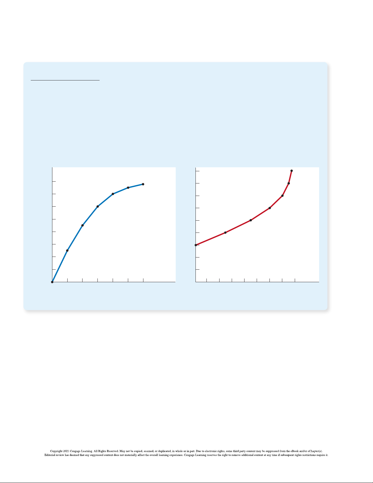
PART V FIRM BEHAVIOR AND THE ORGANIZATION OF INDUSTRY FIGURE 2
The production function in panel (a) shows the relationship between the number of workers
hired and the quantity of output produced. Here the number of workers hired (on the Chloe’s Production Function
horizontal axis) is from column (1) in Table 1, and the quantity of output produced (on and Total-Cost Curve
the vertical axis) is from column (2). The production function gets flatter as the number
of workers increases, reflecting diminishing marginal product. The total-cost curve in
panel (b) shows the relationship between the quantity of output produced and total cost of
production. Here the quantity of output produced (on the horizontal axis) is from column (2)
in Table 1, and the total cost (on the vertical axis) is from column (6). The total-cost curve
gets steeper as the quantity of output increases because of diminishing marginal product. (a) Production function (b) Total-cost curve Quantity Total of Output Cost (cookies $90 per hour) 160 Production 80 Total-cost function curve 140 70 120 60 100 50 80 40 60 30 40 20 20 10 0 1 2 3 4 5 6 Number of 0 20 40 60 80 100 120 140 160 Quantity Workers Hired of Output (cookies per hour)
One of the Ten Principles of Economics in Chapter 1 is that rational people think at
the margin. As we will see in future chapters, this idea is the key to understanding
the decisions a firm makes about how many workers to hire and how much output
to produce. To take a step toward understanding these decisions, column (3) in the marginal product
table gives the marginal product of a worker. The marginal product of any input the increase in output
in the production process is the change in the quantity of output obtained from one that arises from an
additional unit of that input. When the number of workers goes from 1 to 2, cookie additional unit of input
production increases from 50 to 90, so the marginal product of the second worker
is 40 cookies. When the number of workers goes from 2 to 3, cookie production
increases from 90 to 120, so the marginal product of the third worker is 30 cookies.
In the table, the marginal product is shown halfway between two rows because it
represents the change in output as the number of workers increases from one level to another.
Notice that as the number of workers increases, the marginal product declines.
The second worker has a marginal product of 40 cookies, the third worker has a
CHAPTER 13 THE COSTS OF PRODUCTION 249
marginal product of 30 cookies, and the fourth worker has a marginal product of
20 cookies. This property is called diminishing marginal product. At first, when diminishing marginal
only a few workers are hired, they have easy access to Chloe’s kitchen equipment. product
As the number of workers increases, additional workers have to share equipment the property whereby
and work in more crowded conditions. Eventually, the kitchen becomes so over- the marginal product
crowded that workers often get in each other’s way. Hence, as more workers are of an input declines as
hired, each extra worker contributes fewer additional cookies to total production. the quantity of the input
Diminishing marginal product is also apparent in Figure 2. The production increases
function’s slope (“rise over run”) tells us the change in Chloe’s output of cookies
(“rise”) for each additional input of labor (“run”). That is, the slope of the produc-
tion function measures the marginal product. As the number of workers increases,
the marginal product declines, and the production function becomes flatter.
13-2b From the Production Function to the Total-Cost Curve
Columns (4), (5), and (6) in Table 1 show Chloe’s cost of producing cookies. In this
example, the cost of Chloe’s factory is $30 per hour, and the cost of a worker is $10
per hour. If she hires 1 worker, her total cost is $40 per hour. If she hires 2 workers,
her total cost is $50 per hour, and so on. With this information, the table now shows
how the number of workers Chloe hires is related to the quantity of cookies she
produces and to her total cost of production.
Our goal in the next several chapters is to study firms’ production and pricing
decisions. For this purpose, the most important relationship in Table 1 is between
quantity produced [in column (2)] and total cost [in column (6)]. Panel (b) of
Figure 2 graphs these two columns of data with quantity produced on the hori-
zontal axis and total cost on the vertical axis. This graph is called the total-cost curve.
Now compare the total-cost curve in panel (b) with the production function
in panel (a). These two curves are opposite sides of the same coin. The total-cost
curve gets steeper as the amount produced rises, whereas the production func-
tion gets flatter as production rises. These changes in slope occur for the same
reason. High production of cookies means that Chloe’s kitchen is crowded with
many workers. Because the kitchen is crowded, each additional worker adds less
to production, reflecting diminishing marginal product. Therefore, the produc-
tion function is relatively flat. But now turn this logic around: When the kitchen
is crowded, producing an additional cookie requires a lot of additional labor and
is thus very costly. Therefore, when the quantity produced is large, the total-cost curve is relatively steep. QuickQuiz
3. Farmer Greene faces diminishing marginal product.
4. Diminishing marginal product explains why, as a
If she plants no seeds on her farm, she gets no firm’s output increases,
harvest. If she plants 1 bag of seeds, she gets
a. the production function and total-cost curve both
3 bushels of wheat. If she plants 2 bags, she gets get steeper.
5 bushels. If she plants 3 bags, she gets
b. the production function and total-cost curve both a. 6 bushels. get flatter. b. 7 bushels.
c. the production function gets steeper, while the c. 8 bushels. total-cost curve gets flatter. d. 9 bushels.
d. the production function gets flatter, while the total-cost curve gets steeper. Answers at end of chapter. 250
PART V FIRM BEHAVIOR AND THE ORGANIZATION OF INDUSTRY
13-3 The Various Measures of Cost
Our analysis of Chloe’s Cookie Factory showed how a firm’s total cost reflects its
production function. From data on a firm’s total cost, we can derive several related
measures of cost, which we will use to analyze production and pricing decisions
in future chapters. To see how these related measures are derived, we consider
the example in Table 2. This table presents cost data on Chloe’s neighbor—Caleb’s Coffee Shop.
Column (1) in the table shows the number of cups of coffee that Caleb might
produce, ranging from 0 to 10 cups per hour. Column (2) shows Caleb’s total cost
of producing coffee. Figure 3 plots Caleb’s total-cost curve. The quantity of coffee
[from column (1)] is on the horizontal axis, and total cost [from column (2)] is on the
vertical axis. Caleb’s total-cost curve has a shape similar to Chloe’s. In particular,
it becomes steeper as the quantity produced rises, which (as we have discussed)
reflects diminishing marginal product. TABLE 2 (1) (2) (3) (4) (5) (6) (7) (8) Output The Various Measures of (cups of Average Average Average Cost: Caleb’s Coffee Shop coffee per Total Fixed Variable Fixed Variable Total Marginal hour) Cost Cost Cost Cost Cost Cost Cost 0 $3.00 $3.00 $0.00 — — — $0.30 1 3.30 3.00 0.30 $3.00 $0.30 $3.30 0.50 2 3.80 3.00 0.80 1.50 0.40 1.90 0.70 3 4.50 3.00 1.50 1.00 0.50 1.50 0.90 4 5.40 3.00 2.40 0.75 0.60 1.35 1.10 5 6.50 3.00 3.50 0.60 0.70 1.30 1.30 6 7.80 3.00 4.80 0.50 0.80 1.30 1.50 7 9.30 3.00 6.30 0.43 0.90 1.33 1.70 8 11.00 3.00 8.00 0.38 1.00 1.38 1.90 9 12.90 3.00 9.90 0.33 1.10 1.43 2.10 10 15.00 3.00 12.00 0.30 1.20 1.50
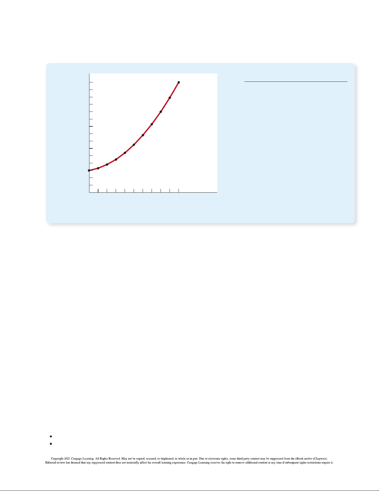
CHAPTER 13 THE COSTS OF PRODUCTION 251 Total Cost FIGURE 3 $15 Total-cost curve 14 Caleb’s Total-Cost Curve 13
Here the quantity of output produced (on
the horizontal axis) is from column (1) in 12
Table 2, and the total cost (on the vertical 11
axis) is from column (2). As in Figure 2, the 10
total-cost curve gets steeper as the quantity 9
of output increases because of diminishing 8 marginal product. 7 6 5 4 3 2 1 0 1 2 3 4 5 6 7 8 9 10 Quantity of Output (cups of coffee per hour) 13-3a Fixed and Variable Costs
Caleb’s total cost can be divided into two types. Some costs, called fixed costs, fixed costs
do not vary with the quantity of output produced. They are incurred even if the costs that do not vary
firm produces nothing at all. Caleb’s fixed costs include any rent he pays because with the quantity of
this cost is the same regardless of how much coffee he produces. Similarly, if output produced
Caleb needs to hire a full-time bookkeeper to pay bills, regardless of the quantity
of coffee produced, the bookkeeper’s salary is a fixed cost. The third column in
Table 2 shows Caleb’s fixed cost, which in this example is $3.00.
Some of the firm’s costs, called variable costs, change as the firm alters the variable costs
quantity of output produced. Caleb’s variable costs include the cost of coffee costs that vary with
beans, milk, sugar, and paper cups: The more cups of coffee Caleb makes, the the quantity of output
more of these items he needs to buy. Similarly, if Caleb has to hire more work- produced
ers to make more cups of coffee, the salaries of these workers are variable costs.
Column (4) in the table shows Caleb’s variable cost. The variable cost is 0 if he
produces nothing, $0.30 if he produces 1 cup of coffee, $0.80 if he produces 2 cups, and so on.
A firm’s total cost is the sum of fixed and variable costs. In Table 2, total cost in
column (2) equals fixed cost in column (3) plus variable cost in column (4).
13-3b Average and Marginal Cost
As the owner of his firm, Caleb has to decide how much to produce. When making
this decision, he will want to consider how the level of production affects his firm’s
costs. Caleb might ask his production supervisor the following two questions about the cost of producing coffee:
How much does it cost to make the typical cup of coffee?
How much does it cost to increase production of coffee by 1 cup? 252
PART V FIRM BEHAVIOR AND THE ORGANIZATION OF INDUSTRY
These two questions might seem to have the same answer, but they do not. Both
answers are important for understanding how firms make production decisions.
To find the cost of the typical unit produced, we divide the firm’s costs by
the quantity of output it produces. For example, if the firm produces 2 cups of
coffee per hour, its total cost is $3.80, and the cost of the typical cup is $3.80/2, average total cost
or $1.90. Total cost divided by the quantity of output is called average total total cost divided by the
cost. Because total cost is the sum of fixed and variable costs, average total cost quantity of output
can be expressed as the sum of average fixed cost and average variable cost.
Average fixed cost equals the fixed cost divided by the quantity of output, and average fixed cost
average variable cost equals the variable cost divided by the quantity of output. fixed cost divided by the
Average total cost tells us the cost of the typical unit, but it does not tell us how quantity of output
much total cost will change as the firm alters its level of production. Column (8) in average variable cost
Table 2 shows the amount that total cost rises when the firm increases production by variable cost divided by
1 unit of output. This number is called marginal cost. For example, if Caleb increases the quantity of output
production from 2 to 3 cups, total cost rises from $3.80 to $4.50, so the marginal cost
of the third cup of coffee is $4.50 minus $3.80, or $0.70. In the table, the marginal marginal cost
cost appears halfway between any two rows because it represents the change in the increase in total cost
total cost as quantity of output increases from one level to another. that arises from an extra
It is helpful to express these definitions mathematically: unit of production
Average total cost 5 Total cost/Quantity ATC 5 T / C Q, and
Marginal cost 5 Change in total cost/Change in quantity MC 5 DTC D / Q.
Here ∆, the Greek letter delta, represents the change in a variable. These equations
show how average total cost and marginal cost are derived from total cost. Average
total cost tells us the cost of a typical unit of output if total cost is divided evenly over all the
units produced. Marginal cost tells us the increase in total cost that arises from producing
an additional unit of output. In the next chapter, business managers like Caleb need
to keep in mind the concepts of average total cost and marginal cost when deciding
how much of their product to supply to the market.
13-3c Cost Curves and Their Shapes
Just as we found graphs of supply and demand useful when analyzing the behavior
of markets in previous chapters, we will find graphs of average and marginal cost
useful when analyzing the behavior of firms. Figure 4 graphs Caleb’s costs using
the data from Table 2. The horizontal axis measures the quantity the firm produces,
and the vertical axis measures marginal and average costs. The graph shows four
curves: average total cost (ATC), average fixed cost (AFC), average variable cost (AVC), and marginal cost (MC).
The cost curves shown here for Caleb’s Coffee Shop have some features that
are common to the cost curves of many firms in the economy. Let’s examine
three features in particular: the shape of the marginal-cost curve, the shape of the
average-total-cost curve, and the relationship between marginal cost and average total cost.
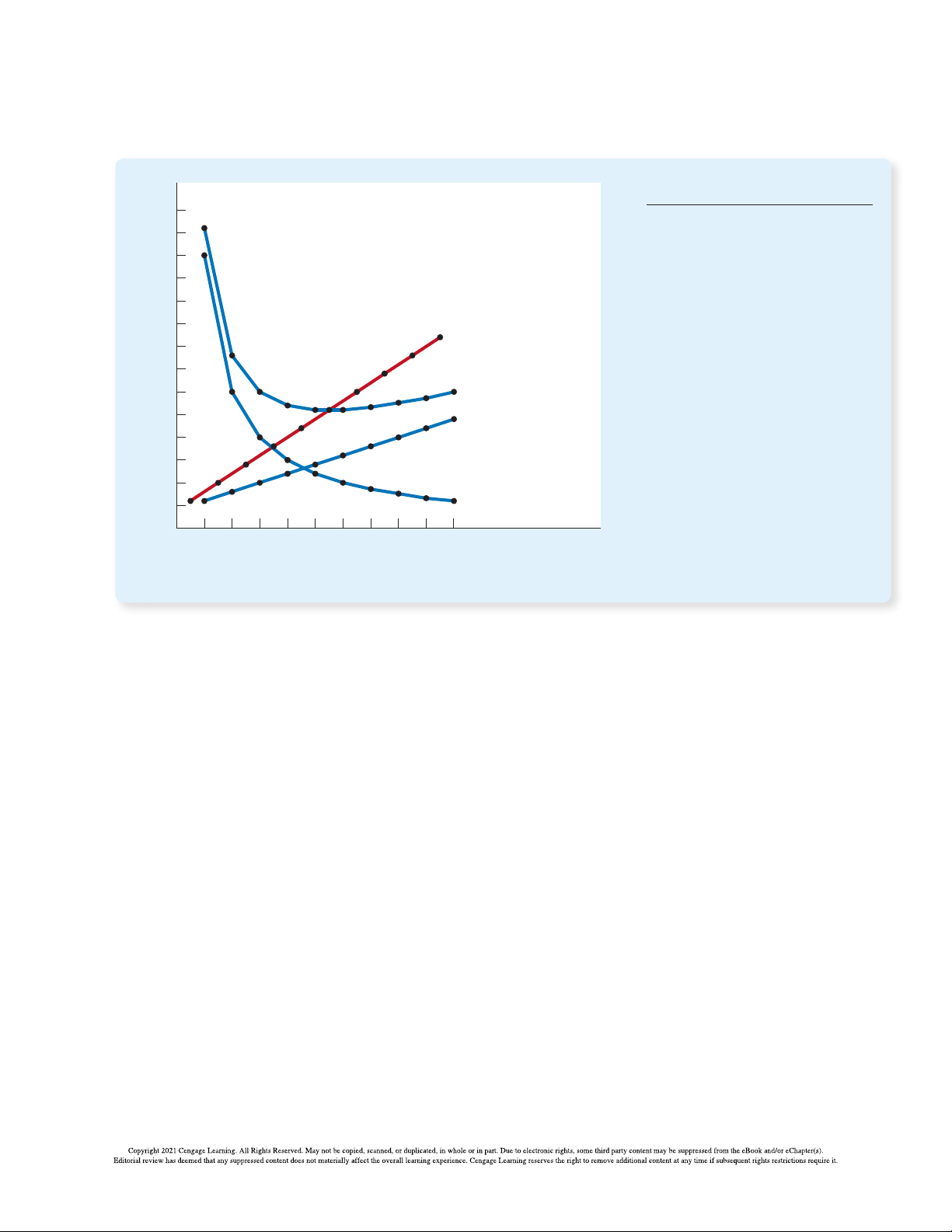
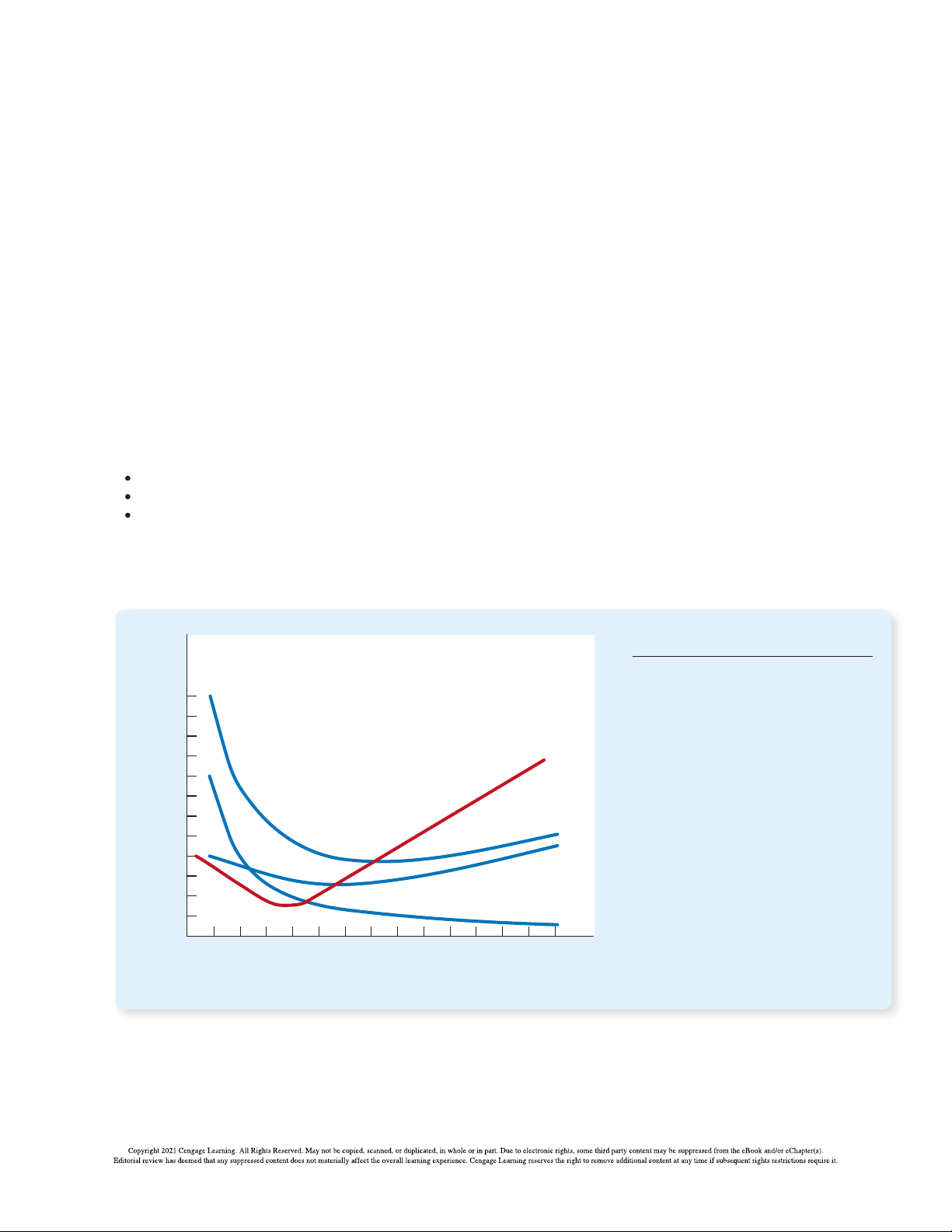
CHAPTER 13 THE COSTS OF PRODUCTION 253 Costs FIGURE 4 $3.50 Caleb’s Average-Cost and 3.25 Marginal-Cost Curves 3.00
This figure shows the average total
cost (ATC), average fixed cost (AFC), 2.75
average variable cost (AVC), and 2.50
marginal cost (MC) for Caleb’s Coffee 2.25
Shop. All of these curves are obtained MC
by graphing the data in Table 2. 2.00
These cost curves show three common 1.75
features: (1) Marginal cost rises 1.50 ATC
with the quantity of output. (2) The
average-total-cost curve is U-shaped. 1.25 AVC
(3) The marginal-cost curve crosses 1.00
the average-total-cost curve at the 0.75 minimum of average total cost. 0.50 0.25 AFC 0 1 2 3 4 5 6 7 8 9 10 Quantity of Output (cups of coffee per hour)
Rising Marginal Cost Caleb’s marginal cost rises as the quantity of output
produced increases. This upward slope reflects the property of diminishing mar-
ginal product. When Caleb produces a small quantity of coffee, he has few work-
ers, and much of his equipment is not used. Because he can easily put these idle
resources to use, the marginal product of an extra worker is large, and the marginal
cost of producing an extra cup of coffee is small. By contrast, when Caleb produces
a large quantity of coffee, his shop is crowded with workers, and most of his equip-
ment is fully utilized. Caleb can produce more coffee by adding workers, but these
new workers have to work in crowded conditions and may have to wait to use the
equipment. Therefore, when the quantity of coffee produced is already high, the
marginal product of an extra worker is low, and the marginal cost of producing an extra cup of coffee is large.
U-Shaped Average Total Cost Caleb’s average-total-cost curve is U-shaped, as
shown in Figure 4. To understand why, remember that average total cost is the sum
of average fixed cost and average variable cost. Average fixed cost always declines
as output rises because the fixed cost is getting spread over a larger number of
units. Average variable cost usually rises as output increases because of diminish- ing marginal product.
Average total cost reflects the shapes of both average fixed cost and average
variable cost. At very low levels of output, such as 1 or 2 cups per hour, average 254
PART V FIRM BEHAVIOR AND THE ORGANIZATION OF INDUSTRY
total cost is very high. Even though average variable cost is low, average fixed cost
is high because the fixed cost is spread over only a few units. As output increases,
the fixed cost is spread over more units. Average fixed cost declines, rapidly at first
and then more slowly. As a result, average total cost also declines until the firm’s
output reaches 5 cups of coffee per hour, when average total cost is $1.30 per cup.
When the firm produces more than 6 cups per hour, however, the increase in aver-
age variable cost becomes the dominant force, and average total cost starts rising.
The tug of war between average fixed cost and average variable cost generates the U-shape in average total cost.
The bottom of the U-shape occurs at the quantity that minimizes average total efficient scale
cost. This quantity is sometimes called the efficient scale of the firm. For Caleb, the quantity of output
the efficient scale is 5 or 6 cups of coffee per hour. If he produces more or less than that minimizes average
this amount, his average total cost rises above the minimum of $1.30. At lower total cost
levels of output, average total cost is higher than $1.30 because the fixed cost is
spread over so few units. At higher levels of output, average total cost is higher
than $1.30 because the marginal product of inputs has diminished significantly.
At the efficient scale, these two forces are balanced to yield the lowest average total cost.
The Relationship between Marginal Cost and Average Total Cost If you
look at Figure 4 (or back at Table 2), you will see something that may be surprising
at first. Whenever marginal cost is less than average total cost, average total cost is falling.
Whenever marginal cost is greater than average total cost, average total cost is rising. This
feature of Caleb’s cost curves is not a coincidence from the particular numbers used
in the example: It is true for all firms.
To see why, consider an analogy. Average total cost is like your cumulative
grade point average. Marginal cost is like the grade you get in the next course you
take. If your grade in your next course is less than your grade point average,
your grade point average will fall. If your grade in your next course is higher
than your grade point average, your grade point average will rise. The mathemat-
ics of average and marginal costs is exactly the same as the mathematics of average and marginal grades.
This relationship between average total cost and marginal cost has an important
corollary: The marginal-cost curve crosses the average-total-cost curve at its minimum.
Why? At low levels of output, marginal cost is below average total cost, so aver-
age total cost is falling. But after the two curves cross, marginal cost rises above
average total cost. As a result, average total cost must start to rise at this level of
output. Hence, this point of intersection is the minimum of average total cost. As
we will see in the next chapter, minimum average total cost plays a key role in the analysis of competitive firms. 13-3d Typical Cost Curves
In the examples we have studied so far, the firms have exhibited diminishing
marginal product and, therefore, rising marginal cost at all levels of output.
This simplifying assumption was useful because it allowed us to focus on
the key features of cost curves that are useful in analyzing firm behavior. Yet
CHAPTER 13 THE COSTS OF PRODUCTION 255
actual firms are often more complex. In many firms, marginal product does
not start to fall immediately after the first worker is hired. Depending on the
production process, the second or third worker might have a higher marginal
product than the first because a team of workers can divide tasks and work
more productively than a single worker. Firms exhibiting this pattern would
experience increasing marginal product for a while before diminishing mar- ginal product set in.
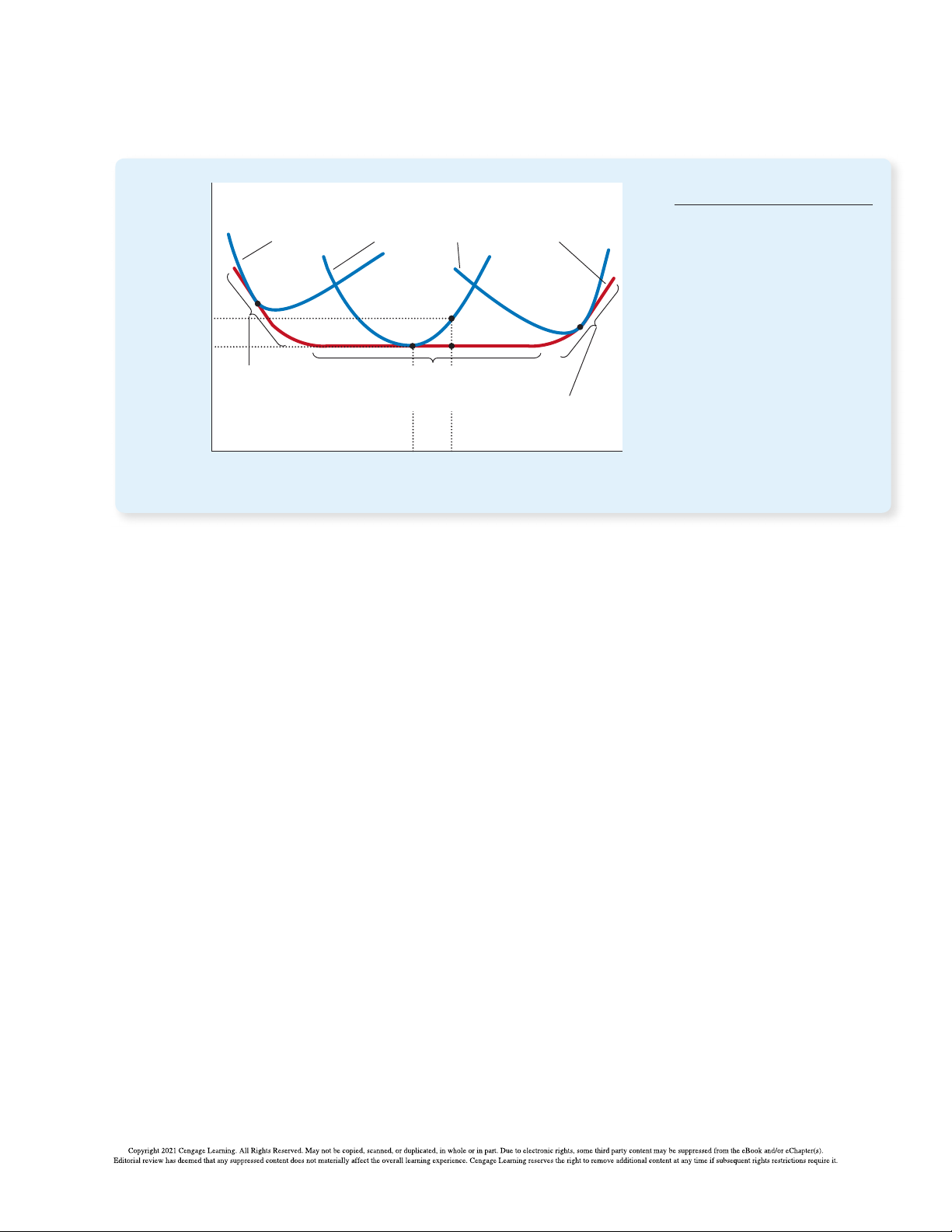
Figure 5 shows the cost curves for such a firm, including average total cost (ATC),
average fixed cost (AFC), average variable cost (AVC), and marginal cost (MC).
At low levels of output, the firm experiences increasing marginal product, and
the marginal-cost curve falls. Eventually, the firm starts to experience diminishing
marginal product, and the marginal-cost curve starts to rise. This combination of
increasing then diminishing marginal product also makes the average-variable-cost curve U-shaped.
Despite these differences from our previous example, the cost curves in Figure 5
share the three properties that are most important to remember:
Marginal cost eventually rises with the quantity of output.
The average-total-cost curve is U-shaped.
The marginal-cost curve crosses the average-total-cost curve at the minimum of average total cost. FIGURE 5 Costs Cost Curves for a Typical Firm
Many firms experience increasing $3.00
marginal product before diminishing
marginal product. As a result, they have 2.50
cost curves shaped like those in this MC
figure. Notice that marginal cost and 2.00
average variable cost fall for a while before starting to rise. 1.50 ATC AVC 1.00 0.50 AFC 0 2 4 6 8 10 12 14 Quantity of Output 256
PART V FIRM BEHAVIOR AND THE ORGANIZATION OF INDUSTRY QuickQuiz
5. A firm is producing 1,000 units at a total cost of
7. The government imposes a $1,000 per year license
$5,000. When it increases production to 1,001 units,
fee on all pizza restaurants. As a result, which cost
its total cost rises to $5,008. For this firm, curves shift?
a. marginal cost is $5, and average variable cost is $8.
a. average total cost and marginal cost
b. marginal cost is $8, and average variable cost is $5.
b. average total cost and average fixed cost
c. marginal cost is $5, and average total cost is $8.
c. average variable cost and marginal cost
d. marginal cost is $8, and average total cost is $5.
d. average variable cost and average fixed cost
6. A firm is producing 20 units with an average
total cost of $25 and a marginal cost of $15. If
it increases production to 21 units, which of the following must occur?
a. Marginal cost will decrease.
b. Marginal cost will increase.
c. Average total cost will decrease.
d. Average total cost will increase. Answers at end of chapter.
13-4 Costs in the Short Run and in the Long Run
Earlier in this chapter, we noted that a firm’s costs might depend on the time
horizon under consideration. Because we want to understand the firm’s decisions
both over the next few days and over the next few years, let’s examine why this is the case.
13-4a The Relationship between Short-Run and Long-Run Average Total Cost
For many firms, the division of total costs between fixed and variable costs depends
on the time horizon. Consider, for instance, a car manufacturer such as Ford Motor
Company. Over a period of only a few months, Ford cannot adjust the number
or sizes of its car factories. The only way it can produce additional cars is to hire
more workers at the factories it already has. The cost of these factories is, therefore,
a fixed cost in the short run. By contrast, over a period of several years, Ford can
expand the size of its factories, build new factories, or close old ones. Thus, the cost
of its factories is a variable cost in the long run.
Because many decisions are fixed in the short run but variable in the long run,
a firm’s long-run cost curves differ from its short-run cost curves. Figure 6 shows
an example. The figure presents three short-run average-total-cost curves—for a
small, medium, and large factory. It also presents the long-run average-total-cost
curve. As the firm moves along the long-run curve, it is adjusting the size of the
factory to the quantity of production.
This graph shows how short-run and long-run costs are related. The long-run
average-total-cost curve has a much flatter U-shape than the short-run average-
total-cost curve. In addition, all the short-run curves lie on or above the long-run
curve. These properties arise because firms have greater flexibility in the long run.
In essence, in the long run, the firm gets to choose which short-run curve it wants.
But in the short run, it has to use whatever short-run curve it has, as determined
by decisions it has made in the past.
The figure shows an example of how a change in production alters costs over
different time horizons. When Ford wants to increase production from 1,000 to
CHAPTER 13 THE COSTS OF PRODUCTION 257 Average FIGURE 6 Total ATC in short ATC in short ATC in short Cost run with run with run with
Average Total Cost in the Short smal factory medium factory large factory ATC in long run and Long Runs
Because fixed costs are variable
in the long run, the average-total-
cost curve in the short run differs
from the average-total-cost curve $12,000 in the long run. 10,000 Economies Constant of returns to scale scale Diseconomies of scale 0 1,000 1,200 Quantity of Cars per Day
1,200 cars per day, it has no choice in the short run but to hire more workers at its
existing medium-sized factory. Because of diminishing marginal product, average
total cost rises from $10,000 to $12,000 per car. In the long run, however, Ford can
expand both the size of the factory and its workforce, and average total cost returns to $10,000.
How long does it take a firm to get to the long run? The answer depends on
the firm. It can take a year or more for a major manufacturing firm, such as a
car company, to build a larger factory. By contrast, a person running a coffee
shop can buy another coffee maker within a few days. There is, therefore, no
single answer to the question of how long it takes a firm to adjust its production facilities.
13-4b Economies and Diseconomies of Scale
The shape of the long-run average-total-cost curve conveys important information economies of scale
about a firm’s production processes. In particular, it tells us how costs vary with the property whereby
the scale—that is, the size—of a firm’s operations. When long-run average total cost long-run average total
declines as output increases, there are said to be economies of scale. When long-run cost falls as the quantity
average total cost rises as output increases, there are said to be diseconomies of of output increases
scale. When long-run average total cost does not vary with the level of output, there
are said to be constant returns to scale. In Figure 6, Ford has economies of scale at diseconomies of scale
low levels of output, constant returns to scale at intermediate levels of output, and the property whereby
diseconomies of scale at high levels of output. long-run average total
What might cause economies or diseconomies of scale? Economies of scale often cost rises as the quantity
arise because higher production levels allow specialization among workers, which of output increases
permits each worker to become better at a specific task. For instance, if Ford hires constant returns to scale
a large number of workers and produces a large number of cars, it can reduce costs the property whereby
using modern assembly-line production. Diseconomies of scale can arise because long-run average total
of coordination problems that often occur in large organizations. The more cars Ford cost stays the same as
produces, the more stretched the management team becomes, and the less effective the quantity of output
the managers become at keeping costs down. changes 258
PART V FIRM BEHAVIOR AND THE ORGANIZATION OF INDUSTRY
This analysis shows why long-run average-total-cost curves are often U-shaped.
At low levels of production, the firm benefits from increased size because it can take
advantage of greater specialization. Coordination problems, meanwhile, are not yet
acute. By contrast, at high levels of production, the benefits of specialization have
already been realized, and coordination problems become more severe as the firm
grows larger. Thus, long-run average total cost is falling at low levels of production
because of increasing specialization and rising at high levels of production because
of growing coordination problems. Lessons from a Pin Factory
“Jack of al trades, master of none.” This old adage sheds light on Smith reported that because of this specialization, the pin factory pro-
the nature of cost curves. A person who tries to do everything usu-
duced thousands of pins per worker every day. He conjectured that if the
al y ends up doing nothing very wel . If a firm wants its workers to be as workers had chosen to work separately, rather than as a team of special-
productive as they can be, it is often best to give each worker a limited ists, “they certainly could not each of them make twenty, perhaps not one
task that she can master. But this organization of work is possible only pin a day.” In other words, because of specialization, a large pin factory
if a firm employs many workers and produces a large quantity of output.
could achieve higher output per worker and lower average cost per pin
In his book The Wealth of Nations, Adam Smith described a visit he than a smal pin factory.
made to a pin factory. Smith was impressed by the specialization among
The specialization that Smith observed in the pin factory is common in
the workers and the resulting economies of scale. He wrote,
the modern economy. If you want to build a house, for instance, you could
try to do all the work yourself. But you would more likely turn to a builder,
One man draws out the wire, another straightens it, a third cuts
who in turn hires carpenters, plumbers, electricians, painters, and many
it, a fourth points it, a fifth grinds it at the top for receiving the
other types of workers. These workers focus their training and experience in
head; to make the head requires two or three distinct operations;
particular jobs, and as a result, they become better at their jobs than if they
to put it on is a peculiar business; to whiten it is another; it is even
were generalists. Indeed, the use of specialization to achieve economies
a trade by itself to put them into paper.
of scale is one reason modern societies are as prosperous as they are. ■ QuickQuiz
8. If a higher level of production allows workers to
9. If Boeing produces 9 jets per month, its long-run
specialize in particular tasks, a firm will likely
total cost is $9 million per month. If it produces
exhibit _________ of scale and _________ average
10 jets per month, its long-run total cost is total cost.
$11 million per month. Boeing exhibits a. economies; falling a. rising marginal cost. b. economies; rising b. falling marginal cost. c. diseconomies; falling c. economies of scale. d. diseconomies; rising d. diseconomies of scale. Answers at end of chapter. 13-5 Conclusion
This chapter has developed some tools to study how firms make production and
pricing decisions. You should now understand what economists mean by the term
costs and how costs vary with the quantity of output a firm produces. To refresh
your memory, Table 3 summarizes some of the definitions we have encountered.
CHAPTER 13 THE COSTS OF PRODUCTION 259
By themselves, a firm’s cost curves do not tell us what decisions the firm will
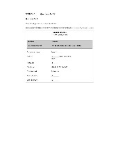
make. But they are a key component of that decision, as we will see in the next chapter. Mathematical TABLE 3 Term Definition Description The Many Types of Explicit costs
Costs that require an outlay of money Cost: A Summary by the firm Implicit costs
Costs that do not require an outlay of money by the firm Fixed costs
Costs that do not vary with the quantity FC of output produced Variable costs
Costs that vary with the quantity of VC output produced Total cost
The market value of all the inputs that TC 5 FC 1 VC a firm uses in production Average fixed cost
Fixed cost divided by the quantity of AFC 5 FC /Q output Average variable cost
Variable cost divided by the quantity of AVC 5 VC /Q output Average total cost
Total cost divided by the quantity of ATC 5 TC /Q output Marginal cost
The increase in total cost that arises MC 5 ∆TC ∆ / Q
from an extra unit of production CHAPTER IN A NUTSHELL
A firm’s goal is to maximize profit, which equals total
produced. Variable costs are costs that change when revenue minus total cost.
the firm alters the quantity of output produced.
When analyzing a firm’s behavior, it is important
From a firm’s total cost, two related measures of cost
to include all the opportunity costs of production.
are derived. Average total cost is total cost divided
Some of the opportunity costs, such as the wages a
by the quantity of output. Marginal cost is the
firm pays its workers, are explicit. Other opportu-
amount by which total cost rises if output increases
nity costs, such as the wages the firm owner gives by 1 unit.
up by working at the firm rather than taking another
When analyzing firm behavior, it is often useful to
job, are implicit. While accounting profit considers
graph average total cost and marginal cost. For a
only explicit costs, economic profit accounts for both
typical firm, marginal cost rises with the quantity explicit and implicit costs.
of output. Average total cost first falls as output
A firm’s costs reflect its production process. A typical
increases and then rises as output increases further.
firm’s production function gets flatter as the quantity
The marginal-cost curve always crosses the average-
of an input increases, displaying the property of dimin-
total-cost curve at the minimum of average total cost.
ishing marginal product. As a result, a firm’s total-cost
A firm’s costs often depend on the time horizon con-
curve gets steeper as the quantity produced rises.
sidered. In particular, many costs are fixed in the short
A firm’s total costs can be separated into its fixed costs
run but variable in the long run. As a result, when the
and its variable costs. Fixed costs are costs that do not
firm changes its level of production, average total cost
change when the firm alters the quantity of output
may rise more in the short run than in the long run. 260
PART V FIRM BEHAVIOR AND THE ORGANIZATION OF INDUSTRY KEY CONCEPTS total revenue, p. 244 production function, p. 247 average variable cost, p. 252 total cost, p. 244 marginal product, p. 248 marginal cost, p. 252 profit, p. 244
diminishing marginal product, p. 249 efficient scale, p. 254 explicit costs, p. 245 fixed costs, p. 251 economies of scale, p. 257 implicit costs, p. 245 variable costs, p. 251 diseconomies of scale, p. 257 economic profit, p. 246 average total cost, p. 252
constant returns to scale, p. 257 accounting profit, p. 246 average fixed cost, p. 252 QUESTIONS FOR REVIEW
1. What is the relationship between a firm’s total
5. Define total cost, average total cost, and marginal cost.
revenue, total cost, and profit? How are they related?
2. Give an example of an opportunity cost that an
6. Draw the marginal-cost and average-total-cost curves
accountant would not count as a cost. Why would the
for a typical firm. Explain why the curves have the accountant ignore this cost?
shapes that they do and why they intersect where
3. What is marginal product, and what is meant by they do. diminishing marginal product?
7. How and why does a firm’s average-total-cost curve
4. Draw a production function that exhibits diminishing
in the short run differ from its average-total-cost
marginal product of labor. Draw the associated curve in the long run?
total-cost curve. (In both cases, be sure to label the
8. Define economies of scale and explain why they might
axes.) Explain the shapes of the two curves you have
arise. Define diseconomies of scale and explain why drawn. they might arise. PROBLEMS AND APPLICATIONS
1. This chapter discusses many types of costs:
c. Buffy thinks she can sell $400,000 worth of
opportunity cost, total cost, fixed cost, variable cost,
amulets in a year. What would her accountant
average total cost, and marginal cost. Fill in the type consider the store’s profit?
of cost that best completes each sentence:
d. Should Buffy open the store? Explain.
a. What you give up in taking some action is called
e. How much revenue would the store need to the _________.
generate for Buffy to earn positive economic
b. _________ is falling when marginal cost is below it profit?
and rising when marginal cost is above it.
3. A commercial fisherman notices the following
c. A cost that does not depend on the quantity
relationship between hours spent fishing and the produced is a(n) _________. quantity of fish caught:
d. In the ice-cream industry in the short run,
_________ includes the cost of cream and sugar Quantity of Fish
but not the cost of the factory. Hours (in pounds)
e. Profits equal total revenue minus _________. 0 hours 0 lb.
f. The cost of producing an extra unit of output is the _________. 1 10
2. Buffy is thinking about opening an amulet store. She 2 18
estimates that it would cost $350,000 per year to rent 3 24
the location and buy the merchandise. In addition, 4 28
she would have to quit her $80,000 per year job as a vampire hunter. 5 30 a. Define opportunity cost.
a. What is the marginal product of each hour spent
b. What is Buffy’s opportunity cost of running the fishing? store for a year?
CHAPTER 13 THE COSTS OF PRODUCTION 261
b. Use these data to graph the fisherman’s
Your current level of production is 600 consoles,
production function. Explain its shape.
all of which have been sold. Someone calls, desperate
c. The fisherman has a fixed cost of $10 (his pole). The
to buy one of your consoles. The caller offers you
opportunity cost of his time is $5 per hour. Graph
$550 for it. Should you accept the offer? Why or
the fisherman’s total-cost curve. Explain its shape. why not?
4. Nimbus, Inc., makes brooms and then sells them
6. Consider the following cost information for a
door-to-door. Here is the relationship between the pizzeria:
number of workers and Nimbus’s output during a Quantity Total Cost Variable Cost given day: 0 dozen pizzas $300 $ 0 Average Marginal Total Total Marginal 1 350 50 Workers Output Product Cost Cost Cost 2 390 90 0 0 ____ ____ 3 420 120 ____ ____ 4 450 150 1 20 ____ ____ 5 490 190 ____ ____ 6 540 240 2 50 ____ ____
a. What is the pizzeria’s fixed cost? ____ ____
b. Construct a table in which you calculate the 3 90 ____ ____
marginal cost per dozen pizzas using the ____ ____
information on total cost. Also, calculate the
marginal cost per dozen pizzas using the 4 120 ____ ____
information on variable cost. What is the ____ ____
relationship between these sets of numbers? 5 140 ____ ____ Explain. ____ ____
7. Your cousin Vinnie owns a painting company with 6 150 ____ ____
fixed costs of $200 and the following schedule for ____ ____ variable costs: 7 155 ____ ____ Quantity of Houses
a. Fill in the column of marginal products. What Painted per
pattern do you see? How might you explain it? Month 1 2 3 4 5 6 7
b. A worker costs $100 a day, and the firm has fixed
costs of $200. Use this information to fill in the
Variable $10 $20 $40 $80 $160 $320 $640 column for total cost. Costs
c. Fill in the column for average total cost. (Recall that ATC 5 T / C Q.) What pattern do you see?
Calculate average fixed cost, average variable cost, and
d. Now fill in the column for marginal cost.
average total cost for each quantity. What is the effi-
(Recall that MC 5 ∆TC/DQ.) What pattern
cient scale of the painting company? do you see?
8. The city government is considering two tax
e. Compare the column for marginal product proposals:
with the column for marginal cost. Explain the
A lump-sum tax of $300 on each producer of relationship. hamburgers.
f. Compare the column for average total cost
A tax of $1 per burger, paid by producers of
with the column for marginal cost. Explain the hamburgers. relationship.
a. Which of the following curves—average fixed
5. You are the chief financial officer for a firm that
cost, average variable cost, average total cost,
sells gaming consoles. Your firm has the following
and marginal cost—would shift as a result of the average-total-cost schedule:
lump-sum tax? Why? Show this in a graph. Label
the graph as precisely as possible. Quantity Average Total Cost
b. Which of these same four curves would shift 600 consoles $300
as a result of the per-burger tax? Why? Show this in a
new graph. Label the graph as precisely as possible. 601 301 262
PART V FIRM BEHAVIOR AND THE ORGANIZATION OF INDUSTRY
9. Jane’s Juice Bar has the following cost schedules:
average-total-cost curve? Between the marginal- Quantity Variable Cost Total Cost
cost curve and the average-variable-cost curve? Explain. 0 vats of juice $ 0 $ 30
10. Consider the following table of long-run total costs 1 10 40 for three different firms: 2 25 55 Quantity 1 2 3 4 5 6 7 3 45 75 Firm A $60 $70 $80 $90 $100 $110 $120 4 70 100 Firm B 11 24 39 56 75 96 119 5 100 130 Firm C 21 34 49 66 85 106 129 6 135 165
Does each of these firms experience economies of scale
a. Calculate average variable cost, average total cost, or diseconomies of scale?
and marginal cost for each quantity.
b. Graph all three curves. What is the relationship
between the marginal-cost curve and the QuickQuiz Answers
1. c 2. a 3. a 4. d 5. d 6. c 7. b 8. a 9. d
Tài liệu liên quan:
-
Test 1 Academic Set - Climate Change Threats to the Great Barrier Reef
16 8 -

Bìa tiếng anh - Bìa tiếng anh UEH
15 8 -
Đề thi tham khảo môn Tiếng Anh 2023 - Sửa đáp án và câu hỏi_test
20 10 -
Module 3, 4, 5 - Tieng Anh: Reducing Relative Clauses & Tenses
16 8 -

Gợi ý đề thi thử TNTHPT năm 2026 môn tiếng anh
28 14