Chapter 4 Decision Analysis | Tài liệu Tiếng Anh

62345_04_ch04_p101-156.qxd 12/23/11 5:25 PM Page 101 CHAPTER 4 Decision Analysis CONTENTS 4.4 RISK ANALYSIS AND 4.1 SENSITIVITY ANALYSIS PROBLEM FORMULATION Risk Analysis Influence Diagrams Sensitivity Analysis Payoff Tables Decision Trees 4.5 DECISION ANALYSIS WITH 4.2 SAMPLE INFORMATION DECISION MAKING Influence Diagram WITHOUT PROBABILITIES Decision Tree Optimistic Approach Decision Strategy Conservative Approach Risk Profile Minimax Regret Approach Expected Value of Sample 4.3 DECISION MAKING WITH Information PROBABILITIES
Efficiency of Sample Information Expected Value of Perfect 4.6 COMPUTING BRANCH Information PROBABILITIES
62345_04_ch04_p101-156.qxd 12/23/11 5:25 PM Page 102 102 Chapter 4 Decision Analysis
Decision analysis can be used to develop an optimal strategy when a decision maker is faced
with several decision alternatives and an uncertain or risk-filled pattern of future events. For
example, Ohio Edison used decision analysis to choose the best type of particulate control
equipment for coal-fired generating units when it faced future uncertainties concerning sul-
fur content restrictions, construction costs, and so on. The State of North Carolina used de-
cision analysis in evaluating whether to implement a medical screening test to detect
metabolic disorders in newborns. The Q.M. in Action, Phytopharm’s New Product Research
and Development, discusses the use of decision analysis to manage Phytopharm’s pipeline
of pharmaceutical products, which have long development times and relatively high levels of uncertainty.
Even when a careful decision analysis has been conducted, the uncertain future events
make the final consequence uncertain. In some cases, the selected decision alternative may
provide good or excellent results. In other cases, a relatively unlikely future event may
occur, causing the selected decision alternative to provide only fair or even poor results. The
risk associated with any decision alternative is a direct result of the uncertainty associated
with the final consequence. A good decision analysis includes careful consideration of risk.
Through risk analysis the decision maker is provided with probability information about the
favorable as well as the unfavorable consequences that may occur.
We begin the study of decision analysis by considering problems that involve reason-
ably few decision alternatives and reasonably few possible future events. Influence dia-
grams and payoff tables are introduced to provide a structure for the decision problem and Q.M. in ACTION
PHYTOPHARM’S NEW PRODUCT RESEARCH AND DEVELOPMENT*
As a pharmaceutical development and functional food
potential and subsequently supporting the negotiation of
company, Phytopharm’s primary revenue streams come
the lump-sum payments for development milestones
from licensing agreements with larger companies. After
and royalties on eventual sales that comprise the licens-
Phytopharm establishes proof of principle for a new ing agreement.
product by successfully completing early clinical trials,
Using computer simulation, the resulting decision
it seeks to reduce its risk by licensing the product to a
analysis model allows Phytopharm to perform sensitiv-
large pharmaceutical or nutrition company that will fur-
ity analysis on estimates of development cost, the prob-
ther develop and market the product.
ability of successful Food & Drug Administration
There is substantial uncertainty regarding the future
clearance, launch date, market size, market share, and
sales potential of early stage products, as only one in ten
patent expiry. In particular, a decision tree model allows
of such products makes it to market and only 30% of
Phytopharm and its licensing partner to mutually agree
these yield a healthy return. Phytopharm and its
upon the number of development milestones. Depend-
licensing partners would often initially propose very
ing on the status of the project at a milestone, the li-
different terms of the licensing agreement. Therefore,
censing partner can opt to abandon the project or
Phytopharm employed a team of researchers to de-
continue development. Laying out these sequential de-
velop a flexible methodology for appraising a product’s
cisions in a decision tree allows Phytopharm to negoti-
ate milestone payments and royalties that equitably
split the project’s value between Phytopharm and its
*Pascale Crama, Bert De Ryck, Zeger Degraeve, and Wang Chong, potential licensee.
“Research and Development Project Valuation and Licensing Negotiations
at Phytopharm plc,” Interfaces, 37 no. 5: 472–487.
62345_04_ch04_p101-156.qxd 12/23/11 5:25 PM Page 103 4.1 Problem Formulation 103
to illustrate the fundamentals of decision analysis. We then introduce decision trees to show
the sequential nature of decision problems. Decision trees are used to analyze more com-
plex problems and to identify an optimal sequence of decisions, referred to as an optimal
decision strategy. Sensitivity analysis shows how changes in various aspects of the problem
affect the recommended decision alternative. 4.1 Problem Formulation
The first step in the decision analysis process is problem formulation. We begin with a ver-
bal statement of the problem. We then identify the decision alternatives; the uncertain
future events, referred to as chance events; and the consequences associated with each com-
bination of decision alternative and chance event outcome. Let us begin by considering a
construction project of the Pittsburgh Development Corporation.
Pittsburgh Development Corporation (PDC) purchased land that will be the site of a
new luxury condominium complex. The location provides a spectacular view of downtown
Pittsburgh and the Golden Triangle, where the Allegheny and Monongahela Rivers meet to
form the Ohio River. PDC plans to price the individual condominium units between $300,000 and $1,400,000.
PDC commissioned preliminary architectural drawings for three different projects:
one with 30 condominiums, one with 60 condominiums, and one with 90 condominiums.
The financial success of the project depends upon the size of the condominium complex
and the chance event concerning the demand for the condominiums. The statement of the
PDC decision problem is to select the size of the new luxury condominium project that
will lead to the largest profit given the uncertainty concerning the demand for the condominiums.
Given the statement of the problem, it is clear that the decision is to select the best size
for the condominium complex. PDC has the following three decision alternatives:
d1 ⫽ a small complex with 30 condominiums
d2 ⫽ a medium complex with 60 condominiums
d3 ⫽ a large complex with 90 condominiums
A factor in selecting the best decision alternative is the uncertainty associated with the
chance event concerning the demand for the condominiums. When asked about the possi-
ble demand for the condominiums, PDC’s president acknowledged a wide range of possi-
bilities but decided that it would be adequate to consider two possible chance event
outcomes: a strong demand and a weak demand.
In decision analysis, the possible outcomes for a chance event are referred to as the
states of nature. The states of nature are defined so they are mutually exclusive (no more
than one can occur) and collectively exhaustive (at least one must occur); thus one and only
one of the possible states of nature will occur. For the PDC problem, the chance event
concerning the demand for the condominiums has two states of nature:
s1 ⫽ strong demand for the condominiums
s2 ⫽ weak demand for the condominiums
Management must first select a decision alternative (complex size); then a state of na-
ture follows (demand for the condominiums) and finally a consequence will occur. In this
case, the consequence is PDC’s profit.
62345_04_ch04_p101-156.qxd 12/23/11 5:25 PM Page 104 104 Chapter 4 Decision Analysis Influence Diagrams
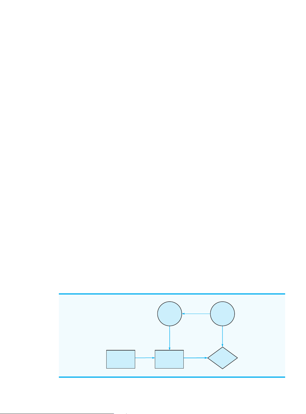
An influence diagram is a graphical device that shows the relationships among the deci-
sions, the chance events, and the consequences for a decision problem. The nodes in an in-
fluence diagram represent the decisions, chance events, and consequences. Rectangles or
squares depict decision nodes, circles or ovals depict chance nodes, and diamonds depict
consequence nodes. The lines connecting the nodes, referred to as arcs, show the direction
of influence that the nodes have on one another. Figure 4.1 shows the influence diagram for
the PDC problem. The complex size is the decision node, demand is the chance node, and
profit is the consequence node. The arcs connecting the nodes show that both the complex
size and the demand influence PDC’s profit. Payoff Tables
Given the three decision alternatives and the two states of nature, which complex size
should PDC choose? To answer this question, PDC will need to know the consequence as-
sociated with each decision alternative and each state of nature. In decision analysis, we re-
fer to the consequence resulting from a specific combination of a decision alternative and
a state of nature as a payoff. A table showing payoffs for all combinations of decision al-
ternatives and states of nature is a payoff table.
Payoffs can be expressed in
Because PDC wants to select the complex size that provides the largest profit, profit is
terms of profit, cost, time,
used as the consequence. The payoff table with profits expressed in millions of dollars is distance, or any other
shown in Table 4.1. Note, for example, that if a medium complex is built and demand turns
measure appropriate for the
out to be strong, a profit of $14 million will be realized. We will use the notation V to de- decision problem being ij analyzed.
note the payoff associated with decision alternative i and state of nature j. Using Table 4.1,
V31 ⫽ 20 indicates a payoff of $20 million occurs if the decision is to build a large complex
(d ) and the strong demand state of nature ( ) occurs. Similarly, 3 s1
V32 ⫽ ⫺9 indicates a loss
of $9 million if the decision is to build a large complex (d ) and the weak demand state of 3 nature (s ) occurs. 2 FIGURE 4.1
INFLUENCE DIAGRAM FOR THE PDC PROJECT States of Nature Strong (s Demand 1) Weak (s2) Complex Profit Size Decision Alternatives Consequence Small complex (d1) Profit Medium complex (d2) Large complex (d3) Cengage Learning 2013 ©
62345_04_ch04_p101-156.qxd 12/23/11 5:25 PM Page 105 4.1 Problem Formulation 105
TABLE 4.1 PAYOFF TABLE FOR THE PDC CONDOMINIUM PROJECT (PAYOFFS IN $ MILLIONS) State of Nature Decision Alternative Strong Demand s Weak Demand 1 s2 Small complex, d 8 7 1 Medium complex, d 14 5 2 Large complex, d 20 3 ⫺9 Cengage Learning 2013 © Decision Trees
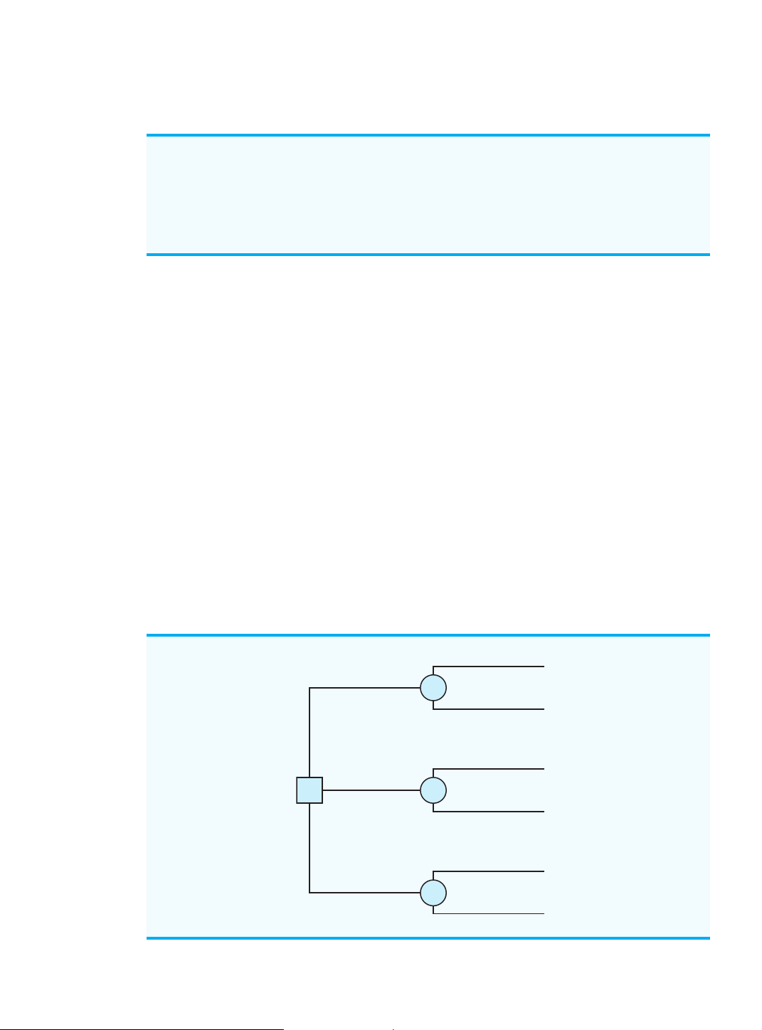
A decision tree provides a graphical representation of the decision-making process. Fig-
ure 4.2 presents a decision tree for the PDC problem. Note that the decision tree shows the
natural or logical progression that will occur over time. First, PDC must make a decision
regarding the size of the condominium complex (d , , or ). Then, after the decision is 1 d2 d3
implemented, either state of nature s or will occur. The number at each endpoint of the 1 s2
tree indicates the payoff associated with a particular sequence. For example, the topmost
payoff of 8 indicates that an $8 million profit is anticipated if PDC constructs a small con-
dominium complex (d ) and demand turns out to be strong ( ). The next payoff of 7 indi- 1 s1
cates an anticipated profit of $7 million if PDC constructs a small condominium complex
(d ) and demand turns out to be weak ( ). Thus, the decision tree provides a graphical de- 1 s2
piction of the sequences of decision alternatives and states of nature that provide the six pos- sible payoffs for PDC.
If you have a payoff table,
The decision tree in Figure 4.2 shows four nodes, numbered 1⫺4. Squares are used to
you can develop a decision
depict decision nodes and circles are used to depict chance nodes. Thus, node 1 is a deci- tree. Try Problem 1, part (a).
sion node, and nodes 2, 3, and 4 are chance nodes. The branches connect the nodes; those
FIGURE 4.2 DECISION TREE FOR THE PDC CONDOMINIUM PROJECT (PAYOFFS IN $ MILLIONS) Strong (s1) 8 Small (d1) 2 Weak (s2) 7 Strong (s1) 14 Medium (d2) 1 3 Weak (s2) 5 Strong (s1) 20 Large (d3) 4 Weak (s2) –9 Cengage Learning 2013 ©
62345_04_ch04_p101-156.qxd 12/23/11 5:25 PM Page 106 106 Chapter 4 Decision Analysis
leaving the decision node correspond to the decision alternatives. The branches leaving each
chance node correspond to the states of nature. The payoffs are shown at the end of the
states-of-nature branches. We now turn to the question: How can the decision maker use the
information in the payoff table or the decision tree to select the best decision alternative?
Several approaches may be used. NOTES AND COMMENTS
1. The first step in solving a complex problem is to
2. People often view the same problem from
decompose the problem into a series of smaller
different perspectives. Thus, the discussion
subproblems. Decision trees provide a useful
regarding the development of a decision tree
way to decompose a problem and illustrate the
may provide additional insight about the
sequential nature of the decision process. problem. 4.2
Decision Making Without Probabilities
In this section we consider approaches to decision making that do not require knowledge
of the probabilities of the states of nature. These approaches are appropriate in situations in
which the decision maker has little confidence in his or her ability to assess the probabili-
ties, or in which a simple best-case and worst-case analysis is desirable. Because different Many people think of a good
decision as one in which the
approaches sometimes lead to different decision recommendations, the decision maker consequence is good.
must understand the approaches available and then select the specific approach that, ac-
However, in some instances,
cording to the judgment of the decision maker, is the most appropriate. a good, well-thought-out decision may still lead to a bad or undesirable Optimistic Approach
consequence while a poor,
The optimistic approach evaluates each decision alternative in terms of the best payoff that ill-conceived decision may still lead to a good or
can occur. The decision alternative that is recommended is the one that provides the best desirable consequence.
possible payoff. For a problem in which maximum profit is desired, as in the PDC problem,
the optimistic approach would lead the decision maker to choose the alternative corre- For a maximization
sponding to the largest profit. For problems involving minimization, this approach leads to problem, the optimistic
choosing the alternative with the smallest payoff.
approach often is referred
To illustrate the optimistic approach, we use it to develop a recommendation for the to as the maximax
PDC problem. First, we determine the maximum payoff for each decision alternative; then approach; for a
we select the decision alternative that provides the overall maximum payoff. These steps minimization problem, the corresponding terminology
systematically identify the decision alternative that provides the largest possible profit. is minimin.
Table 4.2 illustrates these steps.
TABLE 4.2 MAXIMUM PAYOFF FOR EACH PDC DECISION ALTERNATIVE Decision Alternative Maximum Payoff Small complex, d 8 1 Medium complex, d 14 2 Maximum of the Large complex, d 20 3 maximum payoff values Cengage Learning 2013 ©
62345_04_ch04_p101-156.qxd 12/23/11 5:25 PM Page 107 4.2
Decision Making Without Probabilities 107
Because 20, corresponding to d , is the largest payoff, the decision to construct the large 3
condominium complex is the recommended decision alternative using the optimistic approach. Conservative Approach For a maximization
The conservative approach evaluates each decision alternative in terms of the worst pay-
problem, the conservative
off that can occur. The decision alternative recommended is the one that provides the best
approach is often referred to
of the worst possible payoffs. For a problem in which the output measure is profit, as in the
as the maximin approach;
PDC problem, the conservative approach would lead the decision maker to choose the
for a minimization problem,
alternative that maximizes the minimum possible profit that could be obtained. For prob- the corresponding terminology is minimax.
lems involving minimization, this approach identifies the alternative that will minimize the maximum payoff.
To illustrate the conservative approach, we use it to develop a recommendation for the
PDC problem. First, we identify the minimum payoff for each of the decision alternatives;
then we select the decision alternative that maximizes the minimum payoff. Table 4.3 illus-
trates these steps for the PDC problem.
Because 7, corresponding to d , yields the maximum of the minimum payoffs, the de- 1
cision alternative of a small condominium complex is recommended. This decision ap-
proach is considered conservative because it identifies the worst possible payoffs and then
recommends the decision alternative that avoids the possibility of extremely “bad” payoffs.
In the conservative approach, PDC is guaranteed a profit of at least $7 million. Although
PDC may make more, it cannot make less than $7 million. Minimax Regret Approach
In decision analysis, regret is the difference between the payoff associated with a particu-
lar decision alternative and the payoff associated with the decision that would yield the most
desirable payoff for a given state of nature. Thus, regret represents how much potential pay-
off one would forgo by selecting a particular decision alternative given that a specific state
of nature will occur. This is why regret is often referred to as opportunity loss.
As its name implies, under the minimax regret approach to decision making one would
choose the decision alternative that minimizes the maximum state of regret that could occur
over all possible states of nature. This approach is neither purely optimistic nor purely con-
servative. Let us illustrate the minimax regret approach by showing how it can be used to
select a decision alternative for the PDC problem.
Suppose that PDC constructs a small condominium complex (d ) and demand turns 1
out to be strong (s ). Table 4.1 showed that the resulting profit for PDC would be $8 mil- 1
lion. However, given that the strong demand state of nature (s ) has occurred, we realize 1
TABLE 4.3 MINIMUM PAYOFF FOR EACH PDC DECISION ALTERNATIVE Decision Alternative Minimum Payoff Small complex, d 7 Maximum of the 1 minimum payoff values Medium complex, d 5 2 Large complex, d3 ⫺9 Cengage Learning 2013 ©
62345_04_ch04_p101-156.qxd 12/23/11 5:25 PM Page 108 108 Chapter 4 Decision Analysis
TABLE 4.4 OPPORTUNITY LOSS, OR REGRET, TABLE FOR THE PDC CONDOMINIUM PROJECT ($ MILLIONS) State of Nature Decision Alternative Strong Demand s Weak Demand 1 s2 Small complex, d 12 0 1 Medium complex, d 6 2 2 Large complex, d 0 16 3 Cengage Learning 2013 ©
that the decision to construct a large condominium complex (d ), yielding a profit of 3
$20 million, would have been the best decision. The difference between the payoff for the
best decision alternative ($20 million) and the payoff for the decision to construct a small
condominium complex ($8 million) is the regret or opportunity loss associated with deci-
sion alternative d when state of nature occurs; thus, for this case, the opportunity loss 1 s1
or regret is $20 million ⫺ $8 million ⫽ $12 million. Similarly, if PDC makes the decision
to construct a medium condominium complex (d ) and the strong demand state of nature 2
(s ) occurs, the opportunity loss, or regret, associated with would be $20 million 1 d2 ⫺ $14 million ⫽ $6 million.
In general, the following expression represents the opportunity loss, or regret: R *
ij ⫽ 0 Vj ⫺ Vij 0 (4.1) where R and state of nature s
ij ⫽ the regret associated with decision alternative di j V*
j ⫽ the payoff value1 corresponding to the best decision for the state of nature sj V and state of nature s
ij ⫽ the payoff corresponding to decision alternative di j
Note the role of the absolute value in equation (4.1). For minimization problems, the best
payoff, V*, is the smallest entry in column j. Because this value always is less than or equal j
to V , the absolute value of the difference between V* and V ensures that the regret is ij j ij
always the magnitude of the difference.
Using equation (4.1) and the payoffs in Table 4.1, we can compute the regret associated
with each combination of decision alternative d and state of nature s . Because the PDC i j
problem is a maximization problem, V* will be the largest entry in column j of the payoff j
table. Thus, to compute the regret, we simply subtract each entry in a column from the
largest entry in the column. Table 4.4 shows the opportunity loss, or regret, table for the PDC problem.
The next step in applying the minimax regret approach is to list the maximum regret
for each decision alternative; Table 4.5 shows the results for the PDC problem. Selecting
the decision alternative with the minimum of the maximum regret values—hence, the name
minimax regret—yields the minimax regret decision. For the PDC problem, the alternative
to construct the medium condominium complex, with a corresponding maximum regret of
$6 million, is the recommended minimax regret decision.
1In maximization problems, V*j will be the largest entry in column j of the payoff table. In minimization problems, V*j will be
the smallest entry in column j of the payoff table.
62345_04_ch04_p101-156.qxd 12/23/11 5:25 PM Page 109 4.3
Decision Making With Probabilities 109
TABLE 4.5 MAXIMUM REGRET FOR EACH PDC DECISION ALTERNATIVE Decision Alternative Maximum Regret Small complex, d 12 1 Minimum of the Medium complex, d 6 2 maximum regret Large complex, d 16 3 Cengage Learning 2013 ©
For practice in developing
Note that the three approaches discussed in this section provide different recommen-
a decision recommendation
dations, which in itself isn’t bad. It simply reflects the difference in decision-making using the optimistic,
philosophies that underlie the various approaches. Ultimately, the decision maker will have
conservative, and minimax
to choose the most appropriate approach and then make the final decision accordingly. The regret approaches, try Problem 1, part (b).
main criticism of the approaches discussed in this section is that they do not consider any
information about the probabilities of the various states of nature. In the next section we
discuss an approach that utilizes probability information in selecting a decision alternative. 4.3
Decision Making With Probabilities
In many decision-making situations, we can obtain probability assessments for the states of
nature. When such probabilities are available, we can use the expected value approach to
identify the best decision alternative. Let us first define the expected value of a decision
alternative and then apply it to the PDC problem. Let
N ⫽ the number of states of nature P(s )
j ⫽ the probability of state of nature sj
Because one and only one of the N states of nature can occur, the probabilities must satisfy two conditions:
P(sj) ⱖ 0 for all states of nature (4.2) N
a P(sj) ⫽ P(s1) ⫹ P(s2) ⫹ . . . ⫹ P(sN) ⫽ 1 (4.3) j⫽1
The expected value (EV) of decision alternative d is defined as follows: i N
EV(di) ⫽ a P(s j)Vij (4.4) j⫽1
In words, the expected value of a decision alternative is the sum of weighted payoffs for the
decision alternative. The weight for a payoff is the probability of the associated state of na-
ture and therefore the probability that the payoff will occur. Let us return to the PDC prob-
lem to see how the expected value approach can be applied.
PDC is optimistic about the potential for the luxury high-rise condominium complex.
Suppose that this optimism leads to an initial subjective probability assessment of 0.8 that de-
mand will be strong (s ) and a corresponding probability of 0.2 that demand will be weak ( ). 1 s2
62345_04_ch04_p101-156.qxd 12/23/11 5:25 PM Page 110 110 Chapter 4 Decision Analysis Can you now use the Thus, P(s ) )
1 ⫽ 0.8 and P(s2 ⫽ 0.2. Using the payoff values in Table 4.1 and equation (4.4),
expected value approach
we compute the expected value for each of the three decision alternatives as follows: to develop a decision recommendation? Try EV(d ) 1 ⫽ 0.8(8) ⫹ 0.2(7) ⫽ 7.8 Problem 5. EV(d ) 2 ⫽ 0.8(14) ⫹ 0.2(5) ⫽ 12.2 EV(d )
3 ⫽ 0.8(20) ⫹ 0.2(⫺9) ⫽ 14.2
Thus, using the expected value approach, we find that the large condominium complex, with
an expected value of $14.2 million, is the recommended decision.
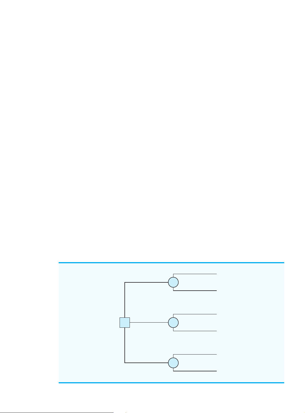
The calculations required to identify the decision alternative with the best expected
value can be conveniently carried out on a decision tree. Figure 4.3 shows the decision tree
for the PDC problem with state-of-nature branch probabilities. Working backward through
the decision tree, we first compute the expected value at each chance node. That is, at each
chance node, we weight each possible payoff by its probability of occurrence. By doing so,
we obtain the expected values for nodes 2, 3, and 4, as shown in Figure 4.4. Computer packages are
Because the decision maker controls the branch leaving decision node 1 and because available to help in
we are trying to maximize the expected profit, the best decision alternative at node 1 is d . 3
constructing more complex
Thus, the decision tree analysis leads to a recommendation of d , with an expected value of 3 decision trees. See
$14.2 million. Note that this recommendation is also obtained with the expected value ap- Appendix 4.1.
proach in conjunction with the payoff table.
Other decision problems may be substantially more complex than the PDC problem,
but if a reasonable number of decision alternatives and states of nature are present, you can
use the decision tree approach outlined here. First, draw a decision tree consisting of deci-
sion nodes, chance nodes, and branches that describe the sequential nature of the problem.
If you use the expected value approach, the next step is to determine the probabilities for
each of the states of nature and compute the expected value at each chance node. Then se-
lect the decision branch leading to the chance node with the best expected value. The deci-
sion alternative associated with this branch is the recommended decision.
The Q.M. in Action, Early Detection of High-Risk Worker Disability Claims, describes
how the Workers’ Compensation Board of British Columbia used a decision tree and ex-
pected cost to help determine whether a short-term disability claim should be considered a high-risk or a low-risk claim.
FIGURE 4.3 PDC DECISION TREE WITH STATE-OF-NATURE BRANCH PROBABILITIES Strong (s1) 8 Small (d1) P(s 2 1) = 0.8 Weak (s2) 7 P(s2) = 0.2 Strong (s1) 14 Medium (d2 ) P(s 1 3 1) = 0.8 Weak (s2) 5 P(s2) = 0.2 Strong (s1) 20 Large (d3) P(s 4 1) = 0.8 Weak (s2) –9 P(s2) = 0.2 Cengage Learning 2013 ©
62345_04_ch04_p101-156.qxd 12/23/11 5:25 PM Page 111 4.3
Decision Making With Probabilities 111
FIGURE 4.4 APPLYING THE EXPECTED VALUE APPROACH USING A DECISION TREE Small (d1) 2
EV(d1) = 0.8(8) + 0.2(7) = $7.8 Medium (d2) 1 3
EV(d2) = 0.8(14) + 0.2(5) = $12.2 Large (d3) 4
EV(d3) = 0.8(20) + 0.2(–9) = $14.2 Cengage Learning 2013 © Q.M. in ACTION
EARLY DETECTION OF HIGH-RISK WORKER DISABILITY CLAIMS*
The Workers’ Compensation Board of British Columbia
process more closely. As a result, WCB could improve the
(WCB) helps workers and employers maintain safe work-
management of the high-risk claims and reduce the cost of
places and helps injured workers obtain disability income
any subsequent long-term disability claims.
and return to work safely. The funds used to make the dis-
The WCB used a decision analysis approach to clas-
ability compensation payments are obtained from assess-
sify each new short-term disability claim as being either a
ments levied on employers. In return, employers receive
high-risk claim or a low-risk claim. A decision tree con-
protection from lawsuits arising from work-related in-
sisting of two decision nodes and two states-of-nature
juries. In recent years, the WCB spent more than $1 bil-
nodes was developed. The two decision alternatives were:
lion on worker compensation and rehabilitation.
(1) Classify the new short-term claim as high-risk and
A short-term disability claim occurs when a worker
intervene; (2) classify the new short-term claim as low-
suffers an injury or illness that results in temporary
risk and do not intervene. The two states of nature were:
absence from work. Whenever a worker fails to recover
(1) The short-term claim converts to a long-term claim;
completely from a short-term disability, the claim is
(2) the short-term claim does not convert to a long-term
reclassified as a long-term disability claim, and more ex-
claim. The characteristics of each new short-term claim
pensive long-term benefits are paid.
were used to determine the probabilities for the states of
The WCB wanted a systematic way to identify short-
nature. The payoffs were the disability claim costs asso-
term disability claims that posed a high financial risk of be-
ciated with each decision alternative and each state-of-
ing converted to the more expensive long-term disability
nature outcome. The objective of minimizing the
claims. If a short-term disability claim could be classified
expected cost determined whether a new short-term claim
as high risk early in the process, a WCB management team
should be classified as high risk.
could intervene and monitor the claim and the recovery
Implementation of the decision analysis model
improved the practice of claim management for the
Workers’ Compensation Board. Early intervention on
*Based on E. Urbanovich, E. Young, M. Puterman, and S. Fattedad, “Early
the high-risk claims saved an estimated $4.7 million
Detection of High-Risk Claims at the Workers’ Compensation Board of
British Columbia,” Interfaces (July/August 2003): 15⫺26. per year.
62345_04_ch04_p101-156.qxd 12/23/11 5:25 PM Page 112 112 Chapter 4 Decision Analysis
Expected Value of Perfect Information
Suppose that PDC has the opportunity to conduct a market research study that would help
evaluate buyer interest in the condominium project and provide information that manage-
ment could use to improve the probability assessments for the states of nature. To determine
the potential value of this information, we begin by supposing that the study could provide
perfect information regarding the states of nature; that is, we assume for the moment that
PDC could determine with certainty, prior to making a decision, which state of nature is go-
ing to occur. To make use of this perfect information, we will develop a decision strategy
that PDC should follow once it knows which state of nature will occur. A decision strategy
is simply a decision rule that specifies the decision alternative to be selected after new information becomes available.
To help determine the decision strategy for PDC, we reproduced PDC’s payoff table as
Table 4.6. Note that, if PDC knew for sure that state of nature s would occur, the best de- 1
cision alternative would be d , with a payoff of $20 million. Similarly, if PDC knew for sure 3
that state of nature s would occur, the best decision alternative would be , with a payoff 2 d1
of $7 million. Thus, we can state PDC’s optimal decision strategy when the perfect infor-
mation becomes available as follows:
If s , select and receive a payoff of $20 million. 1 d3
If s , select and receive a payoff of $7 million. 2 d1
What is the expected value for this decision strategy? To compute the expected value with
perfect information, we return to the original probabilities for the states of nature: P(s ) 1 ⫽ 0.8 and P(s )
2 ⫽ 0.2. Thus, there is a 0.8 probability that the perfect information will indi-
cate state of nature s , and the resulting decision alternative will provide a $20 million 1 d3
profit. Similarly, with a 0.2 probability for state of nature s , the optimal decision alterna- 2
tive d will provide a $7 million profit. Thus, from equation (4.4) the expected value of the 1
decision strategy that uses perfect information is 0.8(20) ⫹ 0.2(7) ⫽ 17.4.
We refer to the expected value of $17.4 million as the expected value with perfect in- formation (EVwPI).
Earlier in this section we showed that the recommended decision using the expected
value approach is decision alternative d , with an expected value of $14.2 million. Because 3
this decision recommendation and expected value computation were made without the ben-
efit of perfect information, $14.2 million is referred to as the expected value without per- fect information (EVwoPI).
The expected value with perfect information is $17.4 million, and the expected value
without perfect information is $14.2; therefore, the expected value of the perfect informa-
tion (EVPI) is $17.4 ⫺ $14.2 ⫽ $3.2 million. In other words, $3.2 million represents the
additional expected value that can be obtained if perfect information were available about the states of nature.
TABLE 4.6 PAYOFF TABLE FOR THE PDC CONDOMINIUM PROJECT ($ MILLIONS) State of Nature Decision Alternative Strong Demand s Weak Demand 1 s2 Small complex, d 8 7 1 Medium complex, d 14 5 2 Large complex, d 20 3 ⫺9 Cengage Learning 2013 ©
62345_04_ch04_p101-156.qxd 12/23/11 5:25 PM Page 113 4.4
Risk Analysis and Sensitivity Analysis 113 It would be worth $3.2
Generally speaking, a market research study will not provide “perfect” information;
million for PDC to learn
however, if the market research study is a good one, the information gathered might be worth the level of market
a sizable portion of the $3.2 million. Given the EVPI of $3.2 million, PDC might seriously
acceptance before selecting
consider a market survey as a way to obtain more information about the states of nature. a decision alternative.
In general, the expected value of perfect information (EVPI) is computed as follows: EVPI ⫽ 0 EVwPI ⫺ EVwoPI 0 (4.5) where
EVPI ⫽ expected value of perfect information
EVwPI ⫽ expected value with perfect information about the states of nature
EVwoPI ⫽ expected value without perfect information about the states of nature
For practice in determining
Note the role of the absolute value in equation (4.5). For minimization problems, the ex- the expected value of
pected value with perfect information is always less than or equal to the expected value
perfect information, try
without perfect information. In this case, EVPI is the magnitude of the difference between Problem 14.
EVwPI and EVwoPI, or the absolute value of the difference as shown in equation (4.5). NOTES AND COMMENTS
1. We restate the opportunity loss, or regret, table
opportunity loss for each of the three decision
for the PDC problem (see Table 4.4) as follows: alternatives is
EOL(d ) ⫽ 0.8(12) ⫹ 0.2(0) ⫽ 9.6 State of Nature 1 EOL(d )
2 ⫽ 0.8(6) ⫹ 0.2(2) ⫽ 5.2 Strong Weak EOL(d )
3 ⫽ 0.8(0) ⫹ 0.2(16) ⫽ 3.2 Demand Demand Decision
Regardless of whether the decision analysis s1 s2
involves maximization or minimization, the Small complex, d 12 0 1
minimum expected opportunity loss always pro- Medium complex, d 6 2 2
vides the best decision alternative. Thus, with Large complex, d 0 16 3 EOL(d ) is the recommended decision. 3 ⫽ 3.2, d3
In addition, the minimum expected opportunity Using P(s ), ), and the opportunity loss 1 P(s2
loss always is equal to the expected value of per-
values, we can compute the expected opportu-
fect information. That is, EOL(best decision) ⫽
nity loss (EOL) for each decision alternative.
EVPI; for the PDC problem, this value is With P(s ) )
1 ⫽ 0.8 and P(s2 ⫽ 0.2, the expected $3.2 million. 4.4
Risk Analysis and Sensitivity Analysis
Risk analysis helps the decision maker recognize the difference between the expected value
of a decision alternative and the payoff that may actually occur. Sensitivity analysis also
helps the decision maker by describing how changes in the state-of-nature probabilities
and/or changes in the payoffs affect the recommended decision alternative. Risk Analysis
A decision alternative and a state of nature combine to generate the payoff associated with
a decision. The risk profile for a decision alternative shows the possible payoffs along with
their associated probabilities.
62345_04_ch04_p101-156.qxd 12/23/11 5:26 PM Page 114 114 Chapter 4 Decision Analysis
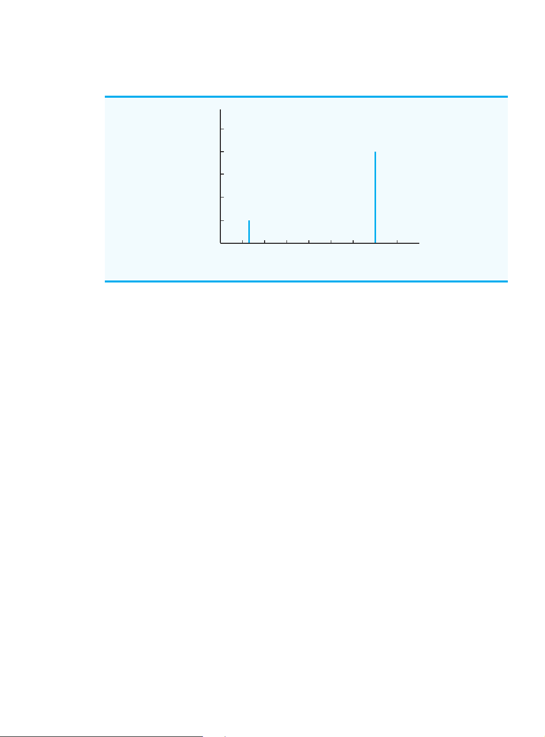
FIGURE 4.5 RISK PROFILE FOR THE LARGE COMPLEX DECISION ALTERNATIVE FOR THE PDC CONDOMINIUM PROJECT 1.0 .8 .6 obability Pr .4 .2 –10 0 10 20 Profit ($ millions) Cengage Learning 2013 ©
Let us demonstrate risk analysis and the construction of a risk profile by returning to
the PDC condominium construction project. Using the expected value approach, we iden-
tified the large condominium complex (d ) as the best decision alternative. The expected 3
value of $14.2 million for d is based on a 0.8 probability of obtaining a $20 million profit 3
and a 0.2 probability of obtaining a $9 million loss. The 0.8 probability for the $20 million
payoff and the 0.2 probability for the ⫺$9 million payoff provide the risk profile for the
large complex decision alternative. This risk profile is shown graphically in Figure 4.5.
Sometimes a review of the risk profile associated with an optimal decision alternative
may cause the decision maker to choose another decision alternative even though the ex-
pected value of the other decision alternative is not as good. For example, the risk profile
for the medium complex decision alternative (d ) shows a 0.8 probability for a $14 million 2
payoff and a 0.2 probability for a $5 million payoff. Because no probability of a loss is as-
sociated with decision alternative d , the medium complex decision alternative would be 2
judged less risky than the large complex decision alternative. As a result, a decision maker
might prefer the less risky medium complex decision alternative even though it has an ex-
pected value of $2 million less than the large complex decision alternative. Sensitivity Analysis
Sensitivity analysis can be used to determine how changes in the probabilities for the states
of nature or changes in the payoffs affect the recommended decision alternative. In many
cases, the probabilities for the states of nature and the payoffs are based on subjective as-
sessments. Sensitivity analysis helps the decision maker understand which of these inputs
are critical to the choice of the best decision alternative. If a small change in the value of
one of the inputs causes a change in the recommended decision alternative, the solution to
the decision analysis problem is sensitive to that particular input. Extra effort and care
should be taken to make sure the input value is as accurate as possible. On the other hand,
if a modest-to-large change in the value of one of the inputs does not cause a change in the
recommended decision alternative, the solution to the decision analysis problem is not sen-
sitive to that particular input. No extra time or effort would be needed to refine the estimated input value.
62345_04_ch04_p101-156.qxd 12/23/11 5:26 PM Page 115 4.4
Risk Analysis and Sensitivity Analysis 115
One approach to sensitivity analysis is to select different values for the probabilities of
the states of nature and the payoffs and then resolve the decision analysis problem. If the
recommended decision alternative changes, we know that the solution is sensitive to the
changes made. For example, suppose that in the PDC problem the probability for a strong
demand is revised to 0.2 and the probability for a weak demand is revised to 0.8. Would the
recommended decision alternative change? Using P(s ) )
1 ⫽ 0.2, P(s2 ⫽ 0.8, and equation
(4.4), the revised expected values for the three decision alternatives are EV(d ) 1 ⫽ 0.2(8) ⫹ 0.8(7) ⫽ 7.2 EV(d ) 2 ⫽ 0.2(14) ⫹ 0.8(5) ⫽ 6.8 EV(d )
3 ⫽ 0.2(20) ⫹ 0.8(⫺9) ⫽ ⫺3.2
With these probability assessments, the recommended decision alternative is to construct a
small condominium complex (d ), with an expected value of $7.2 million. The probability 1
of strong demand is only 0.2, so constructing the large condominium complex (d ) is the 3
least preferred alternative, with an expected value of ⫺$3.2 million (a loss).
Thus, when the probability of strong demand is large, PDC should build the large com-
plex; when the probability of strong demand is small, PDC should build the small complex.
Obviously, we could continue to modify the probabilities of the states of nature and learn
even more about how changes in the probabilities affect the recommended decision alter-
native. The drawback to this approach is the numerous calculations required to evaluate the
effect of several possible changes in the state-of-nature probabilities. Computer software
For the special case of two states of nature, a graphical procedure can be used to deter- packages for decision
mine how changes for the probabilities of the states of nature affect the recommended de-
analysis make it easy to
cision alternative. To demonstrate this procedure, we let p denote the probability of state of calculate these revised nature s ; that is, ) 1
P(s1 ⫽ p. With only two states of nature in the PDC problem, the proba- scenarios.
bility of state of nature s is 2 P(s ) )
2 ⫽ 1 ⫺ P(s1 ⫽ 1 ⫺ p
Using equation (4.4) and the payoff values in Table 4.1, we determine the expected value
for decision alternative d as follows: 1
EV(d1) ⫽ P(s1)(8) ⫹ P(s2)(7)
⫽ p(8) ⫹ (1 ⫺ p)(7) (4.6)
⫽ 8p ⫹ 7 ⫺ 7p ⫽ p ⫹ 7
Repeating the expected value computations for decision alternatives d and , we obtain 2 d3
expressions for the expected value of each decision alternative as a function of p: EV(d ) 2 ⫽ 9p ⫹ 5 (4.7) EV(d ) 3 ⫽ 29p ⫺ 9 (4.8)
Thus, we have developed three equations that show the expected value of the three decision
alternatives as a function of the probability of state of nature s . 1
We continue by developing a graph with values of p on the horizontal axis and the
associated EVs on the vertical axis. Because equations (4.6), (4.7), and (4.8) are linear equa-
tions, the graph of each equation is a straight line. For each equation, we can obtain the line
62345_04_ch04_p101-156.qxd 12/23/11 5:26 PM Page 116 116 Chapter 4 Decision Analysis
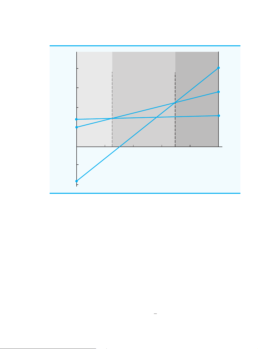
FIGURE 4.6 EXPECTED VALUE FOR THE PDC DECISION ALTERNATIVES AS A FUNCTION OF p d3 provides the highest EV 20 d 3) EV( d 15 2 provides the highest EV d EV(d2) 1 provides the highest EV (EV) 10 alue EV(d1) 5 Expected V 0 p 0.2 0.4 0.6 0.8 1.0 -5 -10 Cengage Learning 2013 ©
by identifying two points that satisfy the equation and drawing a line through the points. For
instance, if we let p ⫽ 0 in equation (4.6), EV(d ) )
1 ⫽ 7. Then, letting p ⫽ 1, EV(d1 ⫽ 8. Con-
necting these two points, (0,7) and (1,8), provides the line labeled EV(d ) in Figure 4.6. Sim- 1
ilarly, we obtain the lines labeled EV(d ) and EV( ); these lines are the graphs of equations 2 d3 (4.7) and (4.8), respectively.
Figure 4.6 shows how the recommended decision changes as p, the probability of the
strong demand state of nature (s ), changes. Note that for small values of 1 p, decision alter-
native d (small complex) provides the largest expected value and is thus the recommended 1
decision. When the value of p increases to a certain point, decision alternative d (medium 2
complex) provides the largest expected value and is the recommended decision. Finally, for
large values of p, decision alternative d (large complex) becomes the recommended 3 decision.
The value of p for which the expected values of d and are equal is the value of 1 d2 p cor-
responding to the intersection of the EV(d ) and the EV( ) lines. To determine this value, 1 d2 we set EV(d ) ) and solve for the value of 1 ⫽ EV(d2 p:
p ⫹ 7 ⫽ 9p ⫹ 5 8p ⫽ 2 2 p ⫽ ⫽ 0.25 8
62345_04_ch04_p101-156.qxd 12/23/11 5:26 PM Page 117 4.4
Risk Analysis and Sensitivity Analysis 117
Hence, when p ⫽ 0.25, decision alternatives d and provide the same expected value. 1 d2
Repeating this calculation for the value of p corresponding to the intersection of the EV(d ) 2
and EV(d ) lines, we obtain 3 p ⫽ 0.70. Graphical sensitivity
Using Figure 4.6, we can conclude that decision alternative d provides the largest ex- 1 analysis shows how
pected value for p ⱕ 0.25, decision alternative d provides the largest expected value for 2 changes in the 0.25 probabilities for the
ⱕ p ⱕ 0.70, and decision alternative d provides the largest expected value for 3 p ⱖ states of nature affect
0.70. Because p is the probability of state of nature s and (1 1
⫺ p) is the probability of state the recommended
of nature s , we now have the sensitivity analysis information that tells us how changes in 2 decision alternative.
the state-of-nature probabilities affect the recommended decision alternative. Try Problem 8.
Sensitivity analysis calculations can also be made for the values of the payoffs. In the
original PDC problem, the expected values for the three decision alternatives were as follows: EV(d ) ) ) (large
1 ⫽ 7.8, EV(d2 ⫽ 12.2, and EV(d3 ⫽ 14.2. Decision alternative d3
complex) was recommended. Note that decision alternative d with EV( ) 2 d2 ⫽ 12.2 was the
second best decision alternative. Decision alternative d will remain the optimal decision 3
alternative as long as EV(d ) is greater than or equal to the expected value of the second 3
best decision alternative. Thus, decision alternative d will remain the optimal decision 3 alternative as long as EV(d ) 3 ⱖ 12.2 (4.9) Let
S ⫽ the payoff of decision alternative d when demand is strong 3
W ⫽ the payoff of decision alternative d when demand is weak 3 Using P(s ) ) ) is
1 ⫽ 0.8 and P(s2 ⫽ 0.2, the general expression for EV(d3 EV(d )
3 ⫽ 0.8S ⫹ 0.2W (4.10)
Assuming that the payoff for d stays at its original value of 3 ⫺$9 million when demand
is weak, the large complex decision alternative will remain optimal as long as EV(d )
3 ⫽ 0.8S ⫹ 0.2(⫺9) ⱖ 12.2 (4.11) Solving for S, we have 0.8S ⫺ 1.8 ⱖ 12.2 0.8S ⱖ 14 S ⱖ 17.5
Recall that when demand is strong, decision alternative d has an estimated payoff of 3
$20 million. The preceding calculation shows that decision alternative d will remain opti- 3
mal as long as the payoff for d when demand is strong is at least $17.5 million. 3
Assuming that the payoff for d when demand is strong stays at its original value of 3
$20 million, we can make a similar calculation to learn how sensitive the optimal solution
is with regard to the payoff for d when demand is weak. Returning to the expected value 3
calculation of equation (4.10), we know that the large complex decision alternative will remain optimal as long as EV(d )
3 ⫽ 0.8(20) ⫹ 0.2W ⱖ 12.2 (4.12)
62345_04_ch04_p101-156.qxd 12/23/11 5:26 PM Page 118 118 Chapter 4 Decision Analysis Solving for W, we have 16 ⫹ 0.2 ⱖ 12.2 0.2W ⱖ ⫺3.8 W ⱖ ⫺19
Recall that when demand is weak, decision alternative d has an estimated payoff of 3
⫺$9 million. The preceding calculation shows that decision alternative d will remain 3
optimal as long as the payoff for d when demand is weak is at least 3 ⫺$19 million.
Based on this sensitivity analysis, we conclude that the payoffs for the large complex
decision alternative (d ) could vary considerably, and would remain the recommended 3 d3
decision alternative. Thus, we conclude that the optimal solution for the PDC decision prob-
lem is not particularly sensitive to the payoffs for the large complex decision alternative.
We note, however, that this sensitivity analysis has been conducted based on only one
Sensitivity analysis can
change at a time. That is, only one payoff was changed and the probabilities for the states assist management in
of nature remained P(s ) )
1 ⫽ 0.8 and P(s2 ⫽ 0.2. Note that similar sensitivity analysis cal- deciding whether
culations can be made for the payoffs associated with the small complex decision alterna-
more time and effort should
tive d and the medium complex decision alternative . However, in these cases, decision
be spent obtaining better 1 d2
estimates of payoffs and
alternative d remains optimal only if the changes in the payoffs for decision alternatives 3 probabilities.
d and meet the requirements that EV( ) ) 1 d2
d1 ⱕ 14.2 and EV(d2 ⱕ 14.2. NOTES AND COMMENTS
1. Some decision analysis software automatically
determine the value of the optimal solution. By
provides the risk profiles for the optimal deci-
varying each input over its range of values, we
sion alternative. These packages also allow the
obtain information about how each input affects
user to obtain the risk profiles for other decision
the value of the optimal solution. To display this
alternatives. After comparing the risk profiles, a
information, a bar is constructed for the input,
decision maker may decide to select a decision
with the width of the bar showing how the input
alternative with a good risk profile even though
affects the value of the optimal solution. The
the expected value of the decision alternative is
widest bar corresponds to the input that is most
not as good as the optimal decision alternative.
sensitive. The bars are arranged in a graph with
2. A tornado diagram, a graphical display, is par-
the widest bar at the top, resulting in a graph that
ticularly helpful when several inputs combine to
has the appearance of a tornado. 4.5
Decision Analysis with Sample Information
In applying the expected value approach, we showed how probability information about the
states of nature affects the expected value calculations and thus the decision recommenda-
tion. Frequently, decision makers have preliminary or prior probability assessments for the
states of nature that are the best probability values available at that time. However, to make
the best possible decision, the decision maker may want to seek additional information
about the states of nature. This new information can be used to revise or update the prior
probabilities so that the final decision is based on more accurate probabilities for the states
of nature. Most often, additional information is obtained through experiments designed to
provide sample information about the states of nature. Raw material sampling, product
testing, and market research studies are examples of experiments (or studies) that may
62345_04_ch04_p101-156.qxd 12/23/11 5:26 PM Page 119 4.5
Decision Analysis with Sample Information 119
enable management to revise or update the state-of-nature probabilities. These revised prob-
abilities are called posterior probabilities.
Let us return to the PDC problem and assume that management is considering a
6-month market research study designed to learn more about potential market acceptance
of the PDC condominium project. Management anticipates that the market research study
will provide one of the following two results:
1. Favorable report: A substantial number of the individuals contacted express inter-
est in purchasing a PDC condominium.
2. Unfavorable report: Very few of the individuals contacted express interest in pur- chasing a PDC condominium. Influence Diagram
By introducing the possibility of conducting a market research study, the PDC problem be-
comes more complex. The influence diagram for the expanded PDC problem is shown in
Figure 4.7. Note that the two decision nodes correspond to the research study and the
complex-size decisions. The two chance nodes correspond to the research study results and
demand for the condominiums. Finally, the consequence node is the profit. From the arcs
of the influence diagram, we see that demand influences both the research study results and
profit. Although demand is currently unknown to PDC, some level of demand for the con-
dominiums already exists in the Pittsburgh area. If existing demand is strong, the research
study is likely to find a substantial number of individuals who express an interest in pur-
chasing a condominium. However, if the existing demand is weak, the research study is
more likely to find a substantial number of individuals who express little interest in pur-
chasing a condominium. In this sense, existing demand for the condominiums will influ-
ence the research study results, and clearly, demand will have an influence upon PDC’s profit.
The arc from the research study decision node to the complex-size decision node indi-
cates that the research study decision precedes the complex-size decision. No arc spans
from the research study decision node to the research study results node because the deci-
sion to conduct the research study does not actually influence the research study results.
The decision to conduct the research study makes the research study results available, but
it does not influence the results of the research study. Finally, the complex-size node and
FIGURE 4.7 INFLUENCE DIAGRAM FOR THE PDC PROBLEM WITH SAMPLE INFORMATION Research Study Demand Results Research Complex Profit Study Size Cengage Learning 2013 ©
62345_04_ch04_p101-156.qxd 12/23/11 5:26 PM Page 120 120 Chapter 4 Decision Analysis
the demand node both influence profit. Note that if a stated cost to conduct the research
study were given, the decision to conduct the research study would also influence profit. In
such a case, we would need to add an arc from the research study decision node to the profit
node to show the influence that the research study cost would have on profit. Decision Tree
The decision tree for the PDC problem with sample information shows the logical sequence
for the decisions and the chance events in Figure 4.8.
First, PDC’s management must decide whether the market research should be con-
ducted. If it is conducted, PDC’s management must be prepared to make a decision about
the size of the condominium project if the market research report is favorable and, possi-
bly, a different decision about the size of the condominium project if the market research
report is unfavorable. In Figure 4.8, the squares are decision nodes and the circles are chance
nodes. At each decision node, the branch of the tree that is taken is based on the decision
made. At each chance node, the branch of the tree that is taken is based on probability or
chance. For example, decision node 1 shows that PDC must first make the decision of
whether to conduct the market research study. If the market research study is undertaken,
chance node 2 indicates that both the favorable report branch and the unfavorable report
branch are not under PDC’s control and will be determined by chance. Node 3 is a decision
node, indicating that PDC must make the decision to construct the small, medium, or large
complex if the market research report is favorable. Node 4 is a decision node showing that
PDC must make the decision to construct the small, medium, or large complex if the mar-
ket research report is unfavorable. Node 5 is a decision node indicating that PDC must make
the decision to construct the small, medium, or large complex if the market research is not
undertaken. Nodes 6 to 14 are chance nodes indicating that the strong demand or weak de-
mand state-of-nature branches will be determined by chance.
Analysis of the decision tree and the choice of an optimal strategy require that we know
the branch probabilities corresponding to all chance nodes. PDC has developed the follow- ing branch probabilities:
If the market research study is undertaken
We explain in Section 4.6
P(Favorable report) ⫽ 0.77
how the branch probabilities
P(Unfavorable report) ⫽ 0.23 for P(Favorable report) and P(Unfavorable report) can
If the market research report is favorable be developed.
P(Strong demand given a favorable report) ⫽ 0.94
P(Weak demand given a favorable report) ⫽ 0.06
If the market research report is unfavorable
P(Strong demand given a favorable report) ⫽ 0.35
P(Weak demand given a favorable report) ⫽ 0.65
If the market research report is not undertaken, the prior probabilities are applicable.
P(Strong demand) ⫽ 0.80 P(Weak demand) ⫽ 0.20
The branch probabilities are shown on the decision tree in Figure 4.9.