1801 - CosFace: Novel Large Margin Cosine Loss for Face Recognition. Môn Mạng máy tính | Đại học Trường Đại học Phenika.
CosFace: Large Margin Cosine Loss for Deep Face Recognition
Hao Wang, Yitong Wang, Zheng Zhou, Xing Ji, Dihong Gong, Jingchao Zhou, Zhifeng Li, and Wei Liu[1] ∗Tencent AI Lab
{hawelwang,yitongwang,encorezhou,denisji,sagazhou,michaelzfli}@tencent.com
gongdihong@gmail.com wliu@ee.columbia.edu
Abstract
Face recognition has made extraordinary progress owing to the advancement of deep convolutional neural networks (CNNs). The central task of face recognition, including face verification and identification, involves face feature discrimination. However, the traditional softmax loss of deep CNNs usually lacks the power of discrimination. To address this problem, recently several loss functions such as center loss, large margin softmax loss, and angular softmax loss have been proposed. All these improved losses
[1] Corresponding authors
1801 - CosFace: Novel Large Margin Cosine Loss for Face Recognition. Môn Mạng máy tính | Đại học Trường Đại học Phenika.
Tài liệu gồm 12 trang giúp bạn tham khảo, củng cố kiến thức và ôn tập đạt kết quả cao trong kỳ thi sắp tới. Mời bạn đọc đón xem!
Môn: Mạng máy tính (Phenikaa) 7 tài liệu
Trường: Đại học Phenika 1.3 K tài liệu
Tác giả:


Preview text:
lOMoAR cPSD| 59561309
CosFace: Large Margin Cosine Loss for Deep Face Recognition
Hao Wang, Yitong Wang, Zheng Zhou, Xing Ji, Dihong Gong, Jingchao Zhou, Zhifeng Li, and Wei Liu1 ∗ Tencent AI Lab
{hawelwang,yitongwang,encorezhou,denisji,sagazhou,michaelzfli}@tencent.com
gongdihong@gmail.com wliu@ee.columbia.edu Abstract
has significantly advanced the state-of-the-art performance on
Face recognition has made extraordinary progress
owing to the advancement of deep convolutional neural
networks (CNNs). The central task of face recognition,
including face verification and identification, involves face
feature discrimination. However, the traditional softmax
loss of deep CNNs usually lacks the power of discrimination.
To address this problem, recently several loss functions
such as center loss, large margin softmax loss, and angular
softmax loss have been proposed. All these improved losses
share the same idea: maximizing inter-class variance and
minimizing intra-class variance. In this paper, we propose
a novel loss function, namely large margin cosine loss
(LMCL), to realize this idea from a different perspective.
More specifically, we reformulate the softmax loss as a
cosine loss by L2 normalizing both features and weight
vectors to remove radial variations, based on which a
Figure 1. An overview of the proposed CosFace framework. In the
cosine margin term is introduced to further maximize the
training phase, the discriminative face features are learned with a
decision margin in the angular space. As a result, minimum
large margin between different classes. In the testing phase, the
intra-class variance and maximum inter-class variance are
testing data is fed into CosFace to extract face features which are
achieved by virtue of normalization and cosine decision
later used to compute the cosine similarity score to perform face
margin maximization. We refer to our model trained with
verification and identification.
LMCL as CosFace. Extensive experimental evaluations are
conducted on the most popular public-domain face
recognition datasets such as MegaFace Challenge, Youtube
a wide variety of computer vision tasks, which makes deep
Faces (YTF) and Labeled Face in the Wild (LFW). We
CNN a dominant machine learning approach for computer
achieve the state-of-the-art performance on these
vision. Face recognition, as one of the most common
benchmarks, which confirms the effectiveness of our
computer vision tasks, has been extensively studied for proposed approach.
decades [37, 45, 22, 19, 20, 40, 2]. Early studies build
shallow models with low-level face features, while modern
face recognition techniques are greatly advanced driven by 1. Introduction
deep CNNs. Face recognition usually includes two sub-
Recently progress on the development of deep
tasks: face verification and face identification. Both of these
convolutional neural networks (CNNs) [15, 18, 12, 9, 44]
two tasks involve three stages: face detection, feature
extraction, and classification. A deep CNN is able to extract 1 Corresponding authors lOMoAR cPSD| 59561309
clean highlevel features, making itself possible to achieve
a difficulty, one has to employ an extra trick with an ad-hoc
superior performance with a relatively simple classification
piecewise function for A-Softmax. More importantly, the architec-
decision margin of A-softmax depends on θ, which leads to
ture: usually, a multilayer perceptron networks followed by
different margins for different classes. As a result, in the
a softmax loss [35, 32]. However, recent studies [42, 24, 23]
decision space, some inter-class features have a larger
found that the traditional softmax loss is insufficient to
margin while others have a smaller margin, which reduces
acquire the discriminating power for classification.
the discriminating power. Unlike A-Softmax, our approach
To encourage better discriminating performance, many
defines the decision margin in the cosine space, thus
research studies have been carried out [42, 5, 7, 10, 39, 23].
avoiding the aforementioned shortcomings.
All these studies share the same idea for maximum
Based on the LMCL, we build a sophisticated deep
discrimination capability: maximizing inter-class variance
model called CosFace, as shown in Figure 1. In the training
and minimizing intra-class variance. For example, [42, 5, 7,
phase, LMCL guides the ConvNet to learn features with a
10, 39] propose to adopt multi-loss learning in order to
large cosine margin. In the testing phase, the face features
increase the feature discriminating power. While these
are extracted from the ConvNet to perform either face
methods improve classification performance over the
verification or face identification. We summarize the
traditional softmax loss, they usually come with some extra
contributions of this work as follows:
limitations. For [42], it only explicitly minimizes the intra-
(1) We embrace the idea of maximizing inter-class
class variance while ignoring the inter-class variances,
variance and minimizing intra-class variance and propose a
which may result in suboptimal solutions. [5, 7, 10, 39]
novel loss function, called LMCL, to learn highly
require thoroughly scheming the mining of pair or triplet
discriminative deep features for face recognition.
samples, which is an extremely time-consuming procedure.
(2) We provide reasonable theoretical analysis based
Very recently, [23] proposed to address this problem from a
on the hyperspherical feature distribution encouraged by
different perspective. More specifically, [23] (A-softmax) LMCL.
projects the original Euclidean space of features to an
(3) The proposed approach advances the state-of-the-
angular space, and introduces an angular margin for larger
art performance over most of the benchmarks on popular inter-class variance.
face databases including LFW[13], YTF[43] and Megaface
Compared to the Euclidean margin suggested by [42, 5, [17,
10], the angular margin is preferred because the cosine of 25].
the angle has intrinsic consistency with softmax. The
formulation of cosine matches the similarity measurement 2. Related Work
that is frequently applied to face recognition. From this
Deep Face Recognition. Recently, face recognition has
perspective, it is more reasonable to directly introduce
achieved significant progress thanks to the great success of
cosine margin between different classes to improve the
deep CNN models [18, 15, 34, 9]. In DeepFace [35] and
cosine-related discriminative information.
DeepID [32], face recognition is treated as a multiclass
In this paper, we reformulate the softmax loss as a cosine
classification problem and deep CNN models are first
loss by L2 normalizing both features and weight vectors to
introduced to learn features on large multi-identities
remove radial variations, based on which a cosine margin
datasets. DeepID2 [30] employs identification and
term m is introduced to further maximize the decision
verification signals to achieve better feature embedding.
margin in the angular space. Specifically, we propose a
Recent works DeepID2+ [33] and DeepID3 [31] further
novel algorithm, dubbed Large Margin Cosine Loss
explore the advanced network structures to boost
(LMCL), which takes the normalized features as input to
recognition performance. FaceNet [29] uses triplet loss to
learn highly discriminative features by maximizing the
learn an Euclidean space embedding and a deep CNN is
inter-class cosine margin. Formally, we define a hyper-
then trained on nearly 200 million face images, leading to
parameter m such that the decision boundary is given by
the state-ofthe-art performance. Other approaches [41, 11]
cos(θ1) − m = cos(θ2), where θi is the angle between the
also prove the effectiveness of deep CNNs on face feature and weight of class recognition. i.
Loss Functions. Loss function plays an important role in
For comparison, the decision boundary of the A-Softmax
deep feature learning. Contrastive loss [5, 7] and triplet loss
is defined over the angular space by cos(mθ1) = cos(θ2),
[10, 39] are usually used to increase the Euclidean margin
which has a difficulty in optimization due to the
for better feature embedding. Wen et al. [42] proposed a
nonmonotonicity of the cosine function. To overcome such lOMoAR cPSD| 59561309
center loss to learn centers for deep features of each identity
where θj is the angle between Wj and x. This formula
and used the centers to reduce intra-class variance. Liu et al.
suggests that both norm and angle of vectors contribute to
[24] proposed a large margin softmax (L-Softmax) by the posterior probability.
adding angular constraints to each identity to improve
To develop effective feature learning, the norm of W
feature discrimination. Angular softmax (A-Softmax) [23]
should be necessarily invariable. To this end, We fix kWjk
improves L-Softmax by normalizing the weights, which
= 1 by L2 normalization. In the testing stage, the face
achieves better performance on a series of open-set face
recognition score of a testing face pair is usually calculated
recognition benchmarks [13, 43, 17]. Other loss functions
according to cosine similarity between the two feature
[47, 6, 4, 3] based on contrastive loss or center loss also
vectors. This suggests that the norm of feature vector x is
demonstrate the performance on enhancing discrimination.
not contributing to the scoring function. Thus, in the
Normalization Approaches. Normalization has been
training stage, we fix kxk = s. Consequently, the posterior
studied in recent deep face recognition studies. [38]
probability merely relies on cosine of angle. The modified
normalizes the weights which replace the inner product with loss can be formulated as
cosine similarity within the softmax loss. [28] applies the L2
constraint on features to embed faces in the normalized
space. Note that normalization on feature vectors or weight . (3)
vectors achieves much lower intra-class angular variability
by concentrating more on the angle during training. Hence
the angles between identities can be well optimized. The
von Mises-Fisher (vMF) based methods [48, 8] and A-
Softmax [23] also adopt normalization in feature learning. 3. Proposed Approach
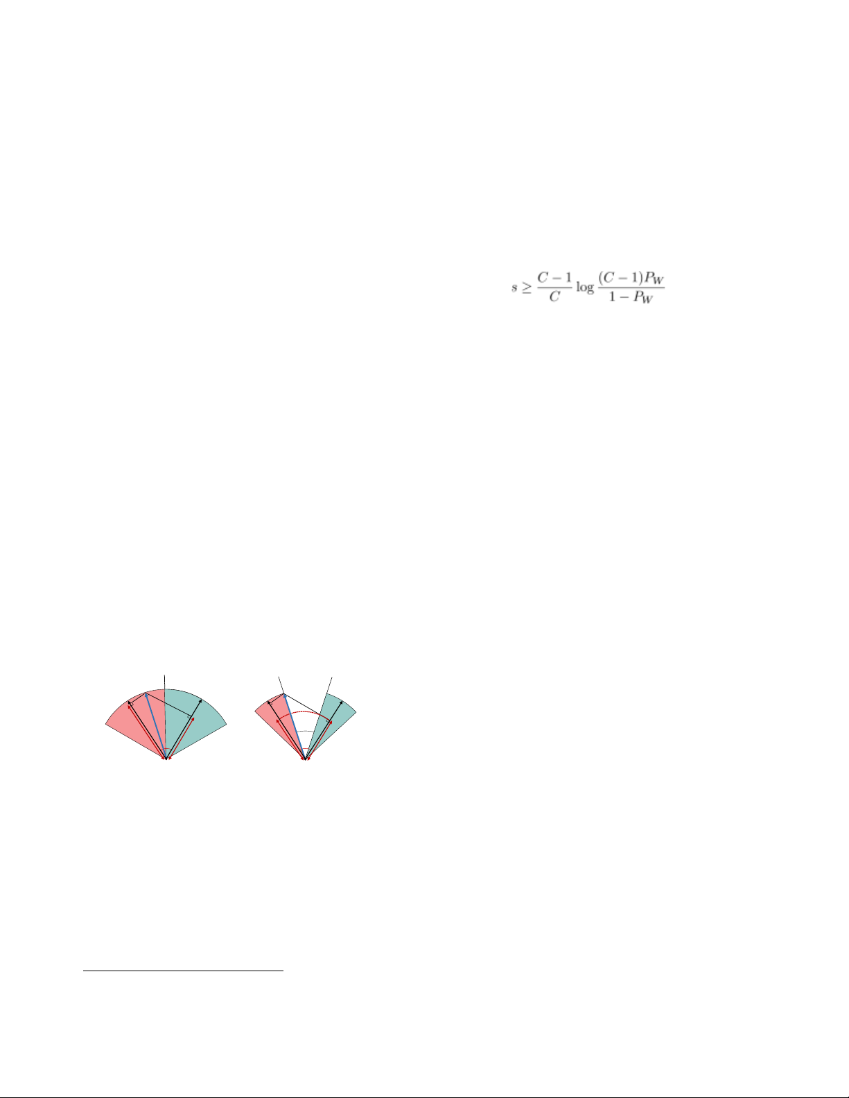
Figure 2. The comparison of decision margins for different loss
functions the binary-classes scenarios. Dashed line represents
In this section, we firstly introduce the proposed LMCL
decision boundary, and gray areas are decision margins.
in detail (Sec. 3.1). And a comparison with other loss
functions is given to show the superiority of the LMCL (Sec.
3.2). The feature normalization technique adopted by the
Because we remove variations in radial directions by fixing
LMCL is further described to clarify its effectiveness (Sec.
kxk = s, the resulting model learns features that are
3.3). Lastly, we present a theoretical analysis for the
separable in the angular space. We refer to this loss as the proposed LMCL (Sec. 3.4).
Normalized version of Softmax Loss (NSL) in this paper. 3.1. Large Margin Cosine Loss
However, features learned by the NSL are not
sufficiently discriminative because the NSL only
We start by rethinking the softmax loss from a cosine
emphasizes correct classification. To address this issue, we
perspective. The softmax loss separates features from
introduce the cosine margin to the classification boundary,
different classes by maximizing the posterior probability of
which is naturally incorporated into the cosine formulation
the ground-truth class. Given an input feature vector xi with of Softmax.
its corresponding label yi, the softmax loss can be
Considering a scenario of binary-classes for example, let formulated as:
θi denote the angle between the learned feature vector and
the weight vector of Class Ci (i = 1,2). The NSL forces
cos(θ1) > cos(θ2) for C1, and similarly for C2, so that
features from different classes are correctly classified. To
where pi denotes the posterior probability of xi being
develop a large margin classifier, we further require
correctly classified. N is the number of training samples and
cos(θ1)−m > cos(θ2) and cos(θ2)−m > cos(θ1), where m ≥
C is the number of classes. fj is usually denoted as activation
0 is a fixed parameter introduced to control the magnitude
of a fully-connected layer with weight vector Wj and bias Bj.
of the cosine margin. Since cos(θi) − m is lower than cos(θi),
We fix the bias Bj = 0 for simplicity, and as a result fj is given
the constraint is more stringent for classification. The above by:
analysis can be well generalized to the scenario of multi- , (2)
classes. Therefore, the altered loss reinforces the
discrimination of learned features by encouraging an extra margin in the cosine space. lOMoAR cPSD| 59561309
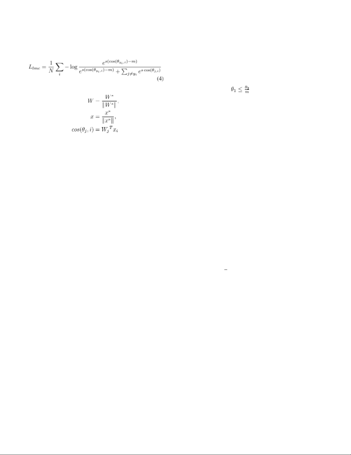
Formally, we define the Large Margin Cosine Loss
A-Softmax improves the softmax loss by introducing an (LMCL) as:
extra margin, such that its decision boundary is given by:
C1 : cos(mθ1) ≥ cos(θ2), C2 : cos(mθ ,
2) ≥ cos(θ1). subject to
Thus, for C1 it requires
, and similarly for C2. The
third subplot of Figure 2 depicts this decision area, where
gray area denotes decision margin. However, the margin of
A-Softmax is not consistent over all θ values: the margin (5)
becomes smaller as θ reduces, and vanishes completely
when θ = 0. This results in two potential issues. First, for ,
difficult classes C1 and C2 which are visually similar and thus
have a smaller angle between W1 and W2, the margin is
where N is the numer of training samples, xi is the i-th
consequently smaller. Second, technically speaking one has
feature vector corresponding to the ground-truth class of yi,
to employ an extra trick with an ad-hoc piecewise function
the Wj is the weight vector of the j-th class, and θj is the
to overcome the nonmonotonicity difficulty of the cosine
angle between Wj and xi. function.
3.2. Comparison on Different Loss Functions
LMCL (our proposed) defines a decision margin in
In this subsection, we compare the decision margin of
cosine space rather than the angle space (like A-Softmax)
our method (LMCL) to: Softmax, NSL, and A-Softmax, as by:
illustrated in Figure 2. For simplicity of analysis, we
C1 : cos(θ1) ≥ cos(θ2) + m, C2 :
consider the binary-classes scenarios with classes C1 and C2.
Let W1 and W2 denote weight vectors for C1 and C2,
cos(θ2) ≥ cos(θ1) + m. respectively.
Softmax loss defines a decision boundary by:
Therefore, cos(θ1) is maximized while cos(θ2) being minimized for C kW
1 (similarly for C2) to perform the large-
1kcos(θ1) = kW2kcos(θ2).
margin classification. The last subplot in Figure 2 illustrates
Thus, its boundary depends on both magnitudes of weight
the decision boundary of LMCL in the cosine space, where
vectors and cosine of angles, which results in an we can
overlapping decision area (margin < 0) in the cosine space.
This is illustrated in the first subplot of Figure 2. As noted
see a clear margin(√2m) in the produced distribution of the
before, in the testing stage it is a common strategy to only
cosine of angle. This suggests that the LMCL is more robust
consider cosine similarity between testing feature vectors of
than the NSL, because a small perturbation around the
faces. Consequently, the trained classifier with the Softmax
decision boundary (dashed line) less likely leads to an
loss is unable to perfectly classify testing samples in the
incorrect decision. The cosine margin is applied cosine space.
consistently to all samples, regardless of the angles of their
NSL normalizes weight vectors W1 and W2 such that they weight vectors.
have constant magnitude 1, which results in a decision boundary given by:
3.3. Normalization on Features cos(θ
In the proposed LMCL, a normalization scheme is 1) = cos(θ2).
involved on purpose to derive the formulation of the cosine
The decision boundary of NSL is illustrated in the second
loss and remove variations in radial directions. Unlike [23]
subplot of Figure 2. We can see that by removing radial
that only normalizes the weight vectors, our approach
variations, the NSL is able to perfectly classify testing
simultaneously normalizes both weight vectors and feature
samples in the cosine space, with margin = 0. However, it is
vectors. As a result, the feature vectors distribute on a
not quite robust to noise because there is no decision margin:
hypersphere, where the scaling parameter s controls the
any small perturbation around the decision boundary can
magnitude of radius. In this subsection, we discuss why change the decision.
feature normalization is necessary and how feature lOMoAR cPSD| 59561309
normalization encourages better feature learning in the
In the following, we show the parameter s should have a proposed LMCL approach.
lower bound to obtain expected classification performance.
The necessity of feature normalization is presented in
Given the normalized learned feature vector x and unit
two respects: First, the original softmax loss without feature
weight vector W, we denote the total number of classes as
normalization implicitly learns both the Euclidean norm
C. Suppose that the learned feature vectors separately lie on
(L2-norm) of feature vectors and the cosine value of the
the surface of the hypersphere and center around the
angle. The L2-norm is adaptively learned for minimizing the
corresponding weight vector. Let PW denote the expected
overall loss, resulting in the relatively weak cosine
minimum posterior probability of class center (i.e., W), the
constraint. Particularly, the adaptive L2-norm of easy
lower bound of s is given by 1:
samples becomes much larger than hard samples to remedy
the inferior performance of cosine metric. On the contrary,
our approach requires the entire set of feature vectors to . (6)
have the same L2-norm such that the learning only depends
Based on this bound, we can infer that s should be
on cosine values to develop the discriminative power.
enlarged consistently if we expect an optimal Pw for
Feature vectors from the same classes are clustered together
classification with a certain number of classes. Besides, by
and those from different classes are pulled apart on the
keeping a fixed Pw, the desired s should be larger to deal
surface of the hypersphere. Additionally, we consider the
with more classes since the growing number of classes
situation when the model initially starts to minimize the
increase the difficulty for classification in the relatively
LMCL. Given a feature vector x, let cos(θi) and cos(θj)
compact space. A hypersphere with large radius s is
denote cosine scores of the two classes, respectively.
therefore required for embedding features with small intra-
Without normalization on features, the LMCL forces
class distance and large inter-class distance.
kxk(cos(θi) − m) > kxkcos(θj). Note that cos(θi) and cos(θj)
can be initially comparable with each other. Thus, as long
3.4. Theoretical Analysis for LMCL
as (cos(θi)−m) is smaller than cos(θj), kxk is required to
The preceding subsections essentially discuss the LMCL
decrease for minimizing the loss, which degenerates the
from the classification point of view. In terms of learning
optimization. Therefore, feature normalization is critical
the discriminative features on the hypersphere, the cosine
under the supervision of LMCL, especially when the
margin servers as momentous part to strengthen the
networks are trained from scratch. Likewise, it is more
discriminating power of features. Detailed analysis about
favorable to fix the scaling parameter s instead of adaptively
the quantitative feasible choice of the cosine margin (i.e., learning.
the bound of hyper-parameter m) is necessary. The optimal
Furthermore, the scaling parameter s should be set to a
choice of m potentially leads to more promising learning of
properly large value to yield better-performing features with
highly discriminative face features. In the following, we
lower training loss. For NSL, the loss continuously goes
delve into the decision boundary and angular margin in the 𝑥 𝑥
feature space to derive the theoretical bound for hyper- 𝑊 1 𝑊2 𝑊 1 𝑊 2 parameter m. Margin
First, considering the binary-classes case with classes C1 cosθ 1 cosθ2 θ 1 θ θ1 θ
and C2 as before, suppose that the normalized feature vector cosθ − m 2 2 1 cosθ2
x is given. Let Wi denote the normalized weight vector, and NSL LMCL
θi denote the angle between x and Wi. For NSL, the decision
boundary defines as cosθ
Figure 3. A geometrical interpretation of LMCL from feature
1 − cosθ2 = 0, which is equivalent
perspective. Different color areas represent feature space from
to the angular bisector of W1 and W2 as shown in the left of
distinct classes. LMCL has a relatively compact feature region
Figure 3. This addresses that the model supervised by NSL compared with NSL.
partitions the underlying feature space to two close regions,
where the features near the boundary are extremely
ambiguous (i.e., belonging to either class is acceptable). In
down with higher s, while too small s leads to an insufficient
contrast, LMCL drives the decision boundary formulated by
convergence even no convergence. For LMCL, we also
cosθ1 − cosθ2 = m for C1, in which θ1 should be much
need adequately large s to ensure a sufficient hyperspace for
smaller than θ2 (similarly for C2). Consequently, the inter-
feature learning with an expected large margin.
1 Proof is attached in the supplemental material. lOMoAR cPSD| 59561309
Figure 4. A toy experiment of different loss functions on 8 identities with 2D features. The first row maps the 2D features onto the Euclidean
space, while the second row projects the 2D features onto the angular space. The gap becomes evident as the margin term m increases.
class variance is enlarged while the intraclass variance shrinks.
Back to Figure 3, one can observe that the maximum
angular margin is subject to the angle between W1 and W2.
Accordingly, the cosine margin should have the limited
variable scope when W1 and W2 are given. Specifically, (7)
suppose a scenario that all the feature vectors belonging to
where C is the number of training classes and K is the
class i exactly overlap with the corresponding weight vector
dimension of learned features. The inequalities indicate that
Wi of class i. In other words, every feature vector is identical
as the number of classes increases, the upper bound of the
to the weight vector for class i, and apparently the feature cosine margin between classes are decreased
space is in an extreme situation, where all the feature
correspondingly. Especially, if the number of classes is
vectors lie at their class center. In that case, the margin of
much larger than the feature dimension, the upper bound of
decision boundaries has been maximized (i.e., the strict
the cosine margin will get even smaller.
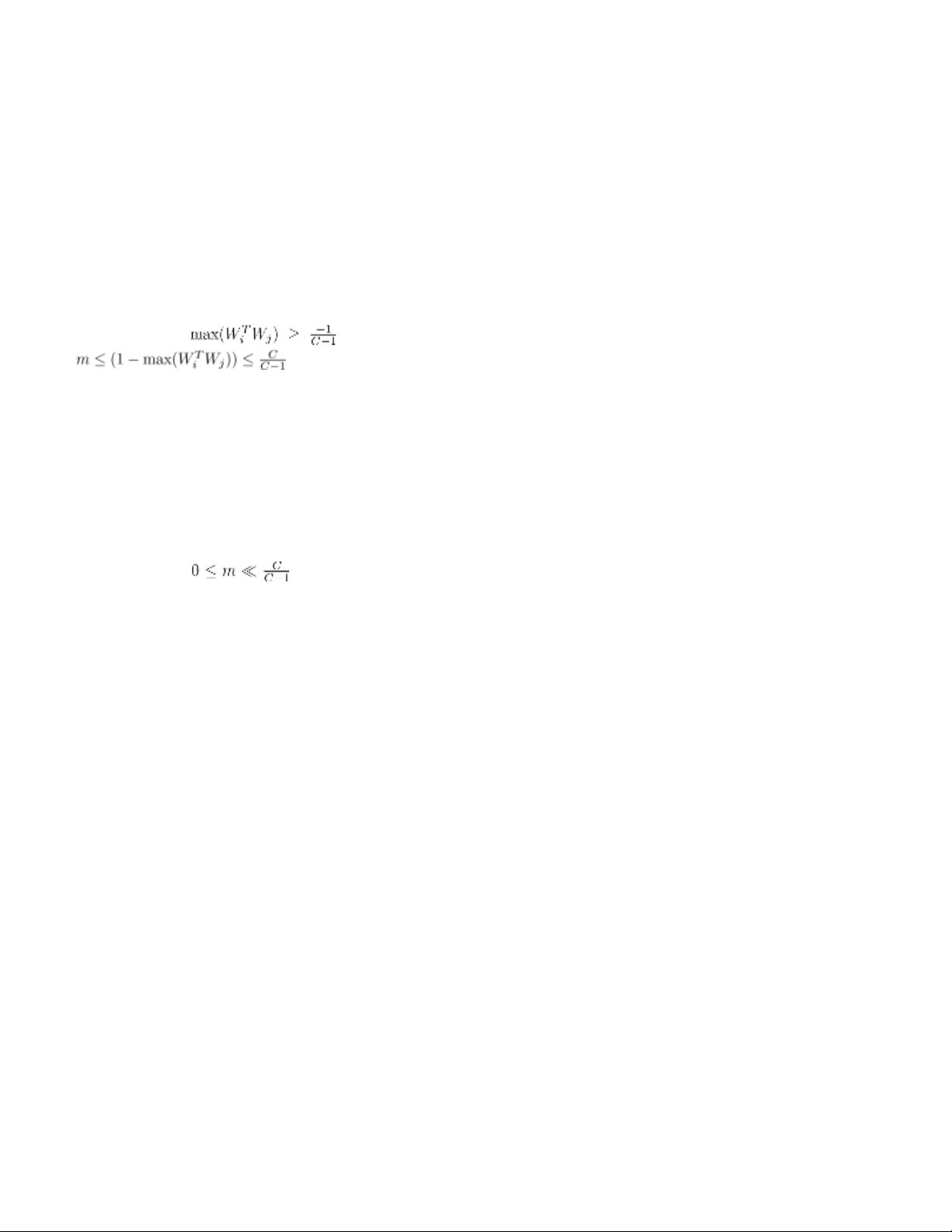
upper bound of the cosine margin). A reasonable choice of larger should
To extend in general, we suppose that all the features are
effectively boost the learning of highly discriminative
well-separated and we have a total number of C classes. The
features. Nevertheless, parameter m usually could not reach
theoretical variable scope of m is supposed to be: 0 ≤ m ≤
the theoretical upper bound in practice due to the vanishing
(1 − max(WiTWj)), where i,j ≤ n,i =6 j.
of the feature space. That is, all the feature vectors are
The softmax loss tries to maximize the angle between any
centered together according to the weight vector of the
of the two weight vectors from two different classes in order
corresponding class. In fact, the model fails to converge
to perform perfect classification. Hence, it is clear that the
when m is too large, because the cosine constraint (i.e.,
optimal solution for the softmax loss should uniformly
cosθ1−m > cosθ2 or cosθ2−m > cosθ1 for two classes)
distribute the weight vectors on a unit hypersphere. Based
becomes stricter and is hard to be satisfied. Besides, the
on this assumption, the variable scope of the introduced
cosine constraint with overlarge m forces the training
cosine margin m can be inferred as follows 1:
process to be more sensitive to noisy data. The ever-
increasing m starts to degrade the overall performance at
some point because of failing to converge.
1 Proof is attached in the supplemental material. lOMoAR cPSD| 59561309
We perform a toy experiment for better visualizing on 100
features and validating our approach. We select face images
from 8 distinct identities containing enough samples to 98
clearly show the feature points on the plot. Several models
are trained using the original softmax loss and the proposed 96
LMCL with different settings of m. We extract 2-D features
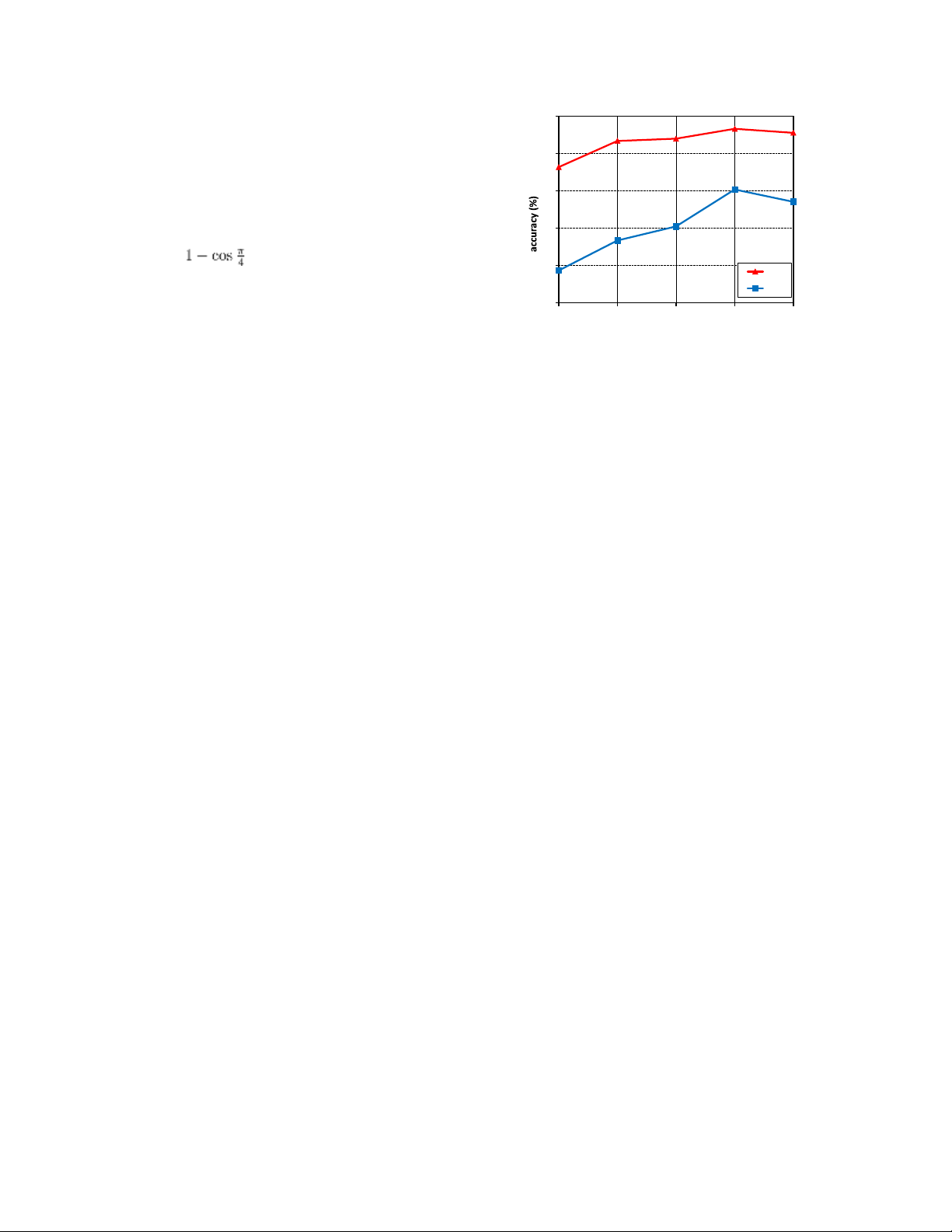
of face images for simplicity. As discussed above, m should 94 be no larger than
(about 0.29), so we set up three 92
choices of m for comparison, which are m = 0, m = 0.1, and LFW
m = 0.2. As shown in Figure 4, the first row and second row YTF 90
present the feature distributions in Euclidean space and 0 0.15 0.25 0.35 0.45
angular space, respectively. We can observe that the original margin
softmax loss produces ambiguity in decision boundaries
while the proposed LMCL performs much better. As m
Figure 5. Accuracy (%) of CosFace with different margin
increases, the angular margin between different classes has
parameters m on LFW[13] and YTF [43]. been amplified. 4. Experiments
models. The CNN models are trained with SGD algorithm, 4.1. Implementation Details
with the batch size of 64 on 8 GPUs. The weight decay is
set to 0.0005. For the case of training on the small dataset,
Preprocessing. Firstly, face area and landmarks are
the learning rate is initially 0.1 and divided by 10 at the 16K,
detected by MTCNN [16] for the entire set of training and
24K, 28k iterations, and we finish the training process at
testing images. Then, the 5 facial points (two eyes, nose and
30k iterations. While the training on the large dataset
two mouth corners) are adopted to perform similarity
terminates at 240k iterations, with the initial learning rate
transformation. After that we obtain the cropped faces
0.05 dropped at 80K, 140K, 200K iterations.
which are then resized to be 112 × 96. Following [42, 23],
Testing. At testing stage, features of original image and
each pixel (in [0, 255]) in RGB images is normalized by
the flipped image are concatenated together to compose the
subtracting 127.5 then dividing by 128.
final face representation. The cosine distance of features is
Training. For a direct and fair comparison to the existing
computed as the similarity score. Finally, face verification
results that use small training datasets (less than 0.5M
and identification are conducted by thresholding and
images and 20K subjects) [17], we train our models on a
ranking the scores. We test our models on several popular
small training dataset, which is the publicly available
public face datasets, including LFW[13], YTF[43], and
CASIAWebFace [46] dataset containing 0.49M face images MegaFace[17, 25].
from 10,575 subjects. We also use a large training dataset to
evaluate the performance of our approach for benchmark 4.2. Exploratory Experiments
comparison with the state-of-the-art results (using large
training dataset) on the benchmark face dataset. The large
Effect of m. The margin parameter m plays a key role in
training dataset that we use in this study is composed of
LMCL. In this part we conduct an experiment to investigate
several public datasets and a private face dataset, containing
the effect of m. By varying m from 0 to 0.45 (If m is larger
about 5M images from more than 90K identities. The
than 0.45, the model will fail to converge), we use the small
training faces are horizontally flipped for data augmentation.
training data (CASIA-WebFace [46]) to train our CosFace
In our experiments we remove face images belong to
model and evaluate its performance on the LFW[13] and
identities that appear in the testing datasets.
YTF[43] datasets, as illustrated in Figure 5. We can see that
For the fair comparison, the CNN architecture used in
the model without the margin (in this case m=0) leads to the
our work is similar to [23], which has 64 convolutional
worst performance. As m being increased, the accuracies
layers and is based on residual units[9]. The scaling
are improved consistently on both datasets, and get
parameter s in Equation (4) is set to 64 empirically. We use
saturated at m = 0.35. This demonstrates the effectiveness
Caffe[14] to implement the modifications of the loss layer
of the margin m. By increasing the margin m, the and run the
discriminative power of the learned features can be
significantly improved. In this study, m is set to fixed 0.35
in the subsequent experiments. lOMoAR cPSD| 59561309
Effect of Feature Normalization. To investigate the effect
evaluate our model strictly following the standard protocol
of the feature normalization scheme in our approach, we
of unrestricted with labeled outside data [13], and report the
train our CosFace models on the CASIA-WebFace with
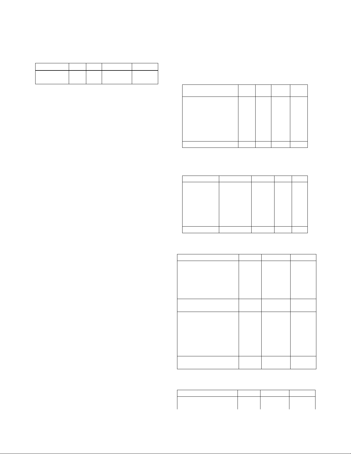
result on the 6,000 pair testing images. YTF [43] contains Normalization LFW YTF MF1 Rank 1 MF1 Veri.
3,425 videos of 1,595 different people. The average length No 99.10 93.1 75.10 88.65
of a video clip is 181.3 frames. All the video sequences were Yes 99.33 96.1 77.11 89.88
downloaded from YouTube. We follow the
Table 1. Comparison of our models with and without feature MF1 Method LFW YTF MF1
normalization on Megaface Challenge 1 (MF1). “Rank 1” refers to Rank1 Veri.
rank-1 face identification accuracy and “Veri.” refers to face Softmax Loss [23] 97.88 93.1 54.85 65.92
verification TAR (True Accepted Rate) under 10−6 FAR (False Softmax+Contrastive [30] 98.78 93.5 65.21 78.86 Accepted Rate). Triplet Loss [29] 98.70 93.4 64.79 78.32 L-Softmax Loss [24] 99.10 94.0 67.12 80.42 Softmax+Center Loss [42] 99.05 94.4 65.49 80.14
and without the feature normalization scheme by fixing m A-Softmax [23] 99.42 95.0 72.72 85.56
to 0.35, and compare their performance on LFW[13], A-Softmax-NormFea 99.32 95.4 75.42 88.82
YTF[43], and the Megaface Challenge 1(MF1)[17]. Note LMCL 99.33 96.1 77.11 89.88
Table 2. Comparison of the proposed LMCL with state-of-the-art
that the model trained without normalization is initialized
loss functions in face recognition community. All the methods in
by softmax loss and then supervised by the proposed LMCL.
this table are using the same training data and the same 64-layer
The comparative results are reported in Table 1. It is very CNN architecture.
clear that the model using the feature normalization scheme Method Training Data #Models LFW YTF
consistently outperforms the model without the feature Deep Face[35] 4M 3 97.35 91.4
normalization scheme across the three datasets. As FaceNet[29] 200M 1 99.63 95.1
discussed above, feature normalization removes radical DeepFR [27] 2.6M 1 98.95 97.3
variance, and the learned features can be more DeepID2+[33] 300K 25 99.47 93.2
discriminative in angular space. This experiment verifies Center Face[42] 0.7M 1 99.28 94.9 this point. Baidu[21] 1.3M 1 99.13 - SphereFace[23] 0.49M 1 99.42 95.0
4.3. Comparison with state-of-the-art loss functions CosFace 5M 1 99.73 97.6
Table 3. Face verification (%) on the LFW and YTF datasets.
In this part, we compare the performance of the proposed
“#Models” indicates the number of models that have been used in
LMCL with the state-of-the-art loss functions. Following the method for evaluation.
the experimental setting in [23], we train a model with the Method Protocol MF1 Rank1 MF1 Veri.
guidance of the proposed LMCL on the CAISAWebFace[46] SIAT MMLAB[42] Small 65.23 76.72
using the same 64-layer CNN architecture described in [23]. DeepSense - Small Small 70.98 82.85
The experimental comparison on LFW, YTF and MF1 are SphereFace - Small[23] Small 75.76 90.04
reported in Table 2. For fair comparison, we are strictly Beijing FaceAll V2 Small 76.66 77.60
following the model structure (a 64-layers ResNet-Like GRCCV Small 77.67 74.88
CNNs) and the detailed experimental settings of FUDAN-CS SDS[41] Small 77.98 79.19
SphereFace [23]. As can be seen in Table 2, LMCL CosFace(Single-patch) Small 77.11 89.88 CosFace(3-patch ensemble) Small 79.54 92.22
consistently achieves competitive results compared to the Beijing FaceAll Norm 1600 Large 64.80 67.11
other losses across the three datasets. Especially, our Google - FaceNet v8[29] Large 70.49 86.47
method not only surpasses the performance of A-Softmax NTechLAB - facenx large Large 73.30 85.08
with feature normalization (named as A-Softmax-NormFea SIATMMLAB TencentVision Large 74.20 87.27
in Table 2), but also significantly outperforms the other loss DeepSense V2 Large 81.29 95.99
functions on YTF and MF1, which demonstrates the YouTu Lab Large 83.29 91.34 effectiveness of LMCL. Vocord - deepVo V3 Large 91.76 94.96 CosFace(Single-patch) Large 82.72 96.65
4.4. Overall Benchmark Comparison CosFace(3-patch ensemble) Large 84.26 97.96
Table 4. Face identification and verification evaluation on MF1. 4.4.1 Evaluation on LFW and YTF
“Rank 1” refers to rank-1 face identification accuracy and “Veri.”
refers to face verification TAR under 10−6 FAR.
LFW [13] is a standard face verification testing dataset in
unconstrained conditions. It includes 13,233 face images Method Protocol MF2 Rank1 MF2 Veri. 3DiVi Large 57.04 66.45
from 5749 identities collected from the website. We Team 2009 Large 58.93 71.12 lOMoAR cPSD| 59561309 NEC Large 62.12 66.84 5. Conclusion GRCCV Large 75.77 74.84 SphereFace Large 71.17 84.22
In this paper, we proposed an innovative approach named CosFace (Single-patch) Large 74.11 86.77
LMCL to guide deep CNNs to learn highly discriminative CosFace(3-patch ensemble) Large 77.06 90.30
face features. We provided a well-formed geometrical and
Table 5. Face identification and verification evaluation on MF2.
theoretical interpretation to verify the effectiveness of the
“Rank 1” refers to rank-1 face identification accuracy and “Veri.”
proposed LMCL. Our approach consistently achieves the
refers to face verification TAR under 10−6 FAR .
state-of-the-art results on several face benchmarks. We wish
unrestricted with labeled outside data protocol and report
that our substantial explorations on learning discriminative
the result on 5,000 video pairs.
features via LMCL will benefit the face recognition
As shown in Table 3, the proposed CosFace achieves community.
state-of-the-art results of 99.73% on LFW and 97.6% on References
YTF. FaceNet achieves the runner-up performance on LFW
[1] FG-NET Aging Database,http://www.fgnet.rsunit.com/. 8
with the large scale of the image dataset, which has
approximately 200 million face images. In terms of YTF,
[2] P. Belhumeur, J. P. Hespanha, and D. Kriegman. Eigenfaces
vs. fisherfaces: Recognition using class specific linear
our model reaches the first place over all other methods.
projection. IEEE Trans. Pattern Analysis and Machine
Intelligence, 19(7):711–720, July 1997. 1
[3] J. Cai, Z. Meng, A. S. Khan, Z. Li, and Y. Tong. Island Loss 4.4.2 Evaluation on MegaFace
for Learning Discriminative Features in Facial Expression
Recognition. arXiv preprint arXiv:1710.03144, 2017. 2
MegaFace [17, 25] is a very challenging testing benchmark
[4] W. Chen, X. Chen, J. Zhang, and K. Huang. Beyond triplet
recently released for large-scale face identification and
loss: a deep quadruplet network for person re-identification.
verification, which contains a gallery set and a probe set.
arXiv preprint arXiv:1704.01719, 2017. 2
The gallery set in Megaface is composed of more than 1
[5] S. Chopra, R. Hadsell, and Y. LeCun. Learning a similarity
million face images. The probe set has two existing
metric discriminatively, with application to face verification.
databases: Facescrub [26] and FGNET [1]. In this study, we
In Conference on Computer Vision and Pattern Recognition
use the Facescrub dataset (containing 106,863 face images (CVPR), 2005. 2
of 530 celebrities) as the probe set to evaluate the
[6] J. Deng, Y. Zhou, and S. Zafeiriou. Marginal loss for deep
performance of our approach on both Megaface Challenge
face recognition. In Conference on Computer Vision and 1 and Challenge
Pattern Recognition Workshops (CVPRW), 2017. 2 2.
[7] R. Hadsell, S. Chopra, and Y. LeCun. Dimensionality
MegaFace Challenge 1 (MF1). On the MegaFace
reduction by learning an invariant mapping. In Conference
Challenge 1 [17], The gallery set incorporates more than 1
on Computer Vision and Pattern Recognition (CVPR), 2006.
million images from 690K individuals collected from Flickr 2
photos [36]. Table 4 summarizes the results of our models
[8] M. A. Hasnat, J. Bohne, J. Milgram, S. Gentric, and L. Chen.
trained on two protocols of MegaFace where the training
von Mises-Fisher Mixture Model-based Deep learning:
dataset is regarded as small if it has less than 0.5 million
Application to Face Verification. arXiv preprint
images, large otherwise. The CosFace approach shows its
arXiv:1706.04264, 2017. 3
superiority for both the identification and verification tasks
[9] K. He, X. Zhang, S. Ren, and J. Sun. Deep Residual Learning on both the protocols.
for Image Recognition. In Conference on Computer Vision
and Pattern Recognition (CVPR), 2016. 1, 2, 6
MegaFace Challenge 2 (MF2). In terms of MegaFace
[10] E. Hoffer and N. Ailon. Deep metric learning using triplet
Challenge 2 [25], all the algorithms need to use the training
network. In International Workshop on Similarity-Based
data provided by MegaFace. The training data for Megaface
Pattern Recognition, 2015. 2
Challenge 2 contains 4.7 million faces and 672K identities,
[11] G. Hu, Y. Yang, D. Yi, J. Kittler, W. Christmas, S. Z. Li, and
which corresponds to the large protocol. The gallery set has
T. Hospedales. When face recognition meets with deep
1 million images that are different from the challenge 1
learning: an evaluation of convolutional neural networks for
gallery set. Not surprisingly, Our method wins the first place
face recognition. In International Conference on Computer
of challenge 2 in table 5, setting a new state-of-the-art with
Vision Workshops (ICCVW), 2015. 2
a large margin (1.39% on rank-1 identification accuracy and
[12] J. Hu, L. Shen, and G. Sun. Squeeze-and-Excitation
5.46% on verification performance).
Networks. arXiv preprint arXiv:1709.01507, 2017. 1 lOMoAR cPSD| 59561309
[13] G. B. Huang, M. Ramesh, T. Berg, and E. Learned-Miller.
[28] R. Ranjan, C. D. Castillo, and R. Chellappa. L2-constrained
Labeled faces in the wild: A database for studying face
Softmax Loss for Discriminative Face Verification. arXiv
recognition in unconstrained environments. In Technical
preprint arXiv:1703.09507, 2017. 2
Report 07-49, University of Massachusetts, Amherst, 2007.
[29] F. Schroff, D. Kalenichenko, and J. Philbin. Facenet: A 2, 7
unified embedding for face recognition and clustering. In
[14] Y. Jia, E. Shelhamer, J. Donahue, S. Karayev, J. Long, R.
Conference on Computer Vision and Pattern Recognition
Girshick, S. Guadarrama, and T. Darrell. Caffe: (CVPR), 2015. 2, 8
Convolutional architecture for fast feature embedding. In
[30] Y. Sun, Y. Chen, X. Wang, and X. Tang. Deep learning face
Proceedings of the 2016 ACM on Multimedia Conference
representation by joint identification-verification. In (ACM MM), 2014. 6
Advances in Neural Information Processing Systems (NIPS),
[15] K. Simonyan and A. Zisserman. Very deep convolutional 2014. 2, 8
networks for large-scale image recognition. In International
[31] Y. Sun, D. Liang, X. Wang, and X. Tang. DeepID3: Face
Conference on Learning Representations (ICLR), 2015. 1, 2
recognition with very deep neural networks. arXiv preprint
[16] K. Zhang, Z. Zhang, Z. Li and Y. Qiao. Joint Face Detection
arXiv:1502.00873, 2015. 2
and Alignment using Multi-task Cascaded Convolutional
[32] Y. Sun, X. Wang, and X. Tang. Deep learning face
Networks. Signal Processing Letters, 23(10):1499– 1503,
representation from predicting 10,000 classes. In Conference 2016. 6
on Computer Vision and Pattern Recognition (CVPR), 2014.
[17] I. Kemelmacher-Shlizerman, S. M. Seitz, D. Miller, and E. 2
Brossard. The megaface benchmark: 1 million faces for
[33] Y. Sun, X. Wang, and X. Tang. Deeply learned face
recognition at scale. In Conference on Computer Vision and
representations are sparse, selective, and robust. In
Pattern Recognition (CVPR), 2016. 2, 6, 7, 8
Conference on Computer Vision and Pattern Recognition
[18] A. Krizhevsky, I. Sutskever, and G. E. Hinton. Imagenet (CVPR), 2015. 2,
classification with deep convolutional neural networks. In 8
Advances in Neural Information Processing Systems (NIPS),
[34] C. Szegedy, W. Liu, Y. Jia, P. Sermanet, S. Reed, D. Anguelov, 2012. 1, 2
D. Erhan, V. Vanhoucke, and A. Rabinovich. Going deeper
[19] Z. Li, D. Lin, and X. Tang. Nonparametric discriminant
with convolutions. In Conference on Computer Vision and
analysis for face recognition. IEEE Transactions on Pattern
Pattern Recognition (CVPR), 2015. 2
Analysis and Machine Intelligence, 31:755–761, 2009. 1
[35] Y. Taigman, M. Yang, M. Ranzato, and L. Wolf. Deepface:
[20] Z. Li, W. Liu, D. Lin, and X. Tang. Nonparametric subspace
Closing the gap to human-level performance in face
analysis for face recognition. In Conference on Computer
verification. In Conference on Computer Vision and Pattern
Vision and Pattern Recognition (CVPR), 2005. 1
Recognition (CVPR), 2014. 2, 8
[21] J. Liu, Y. Deng, T. Bai, Z. Wei, and C. Huang. Targeting
[36] B. Thomee, D. A. Shamma, G. Friedland, B. Elizalde, K. Ni,
ultimate accuracy: Face recognition via deep embedding.
D. Poland, D. Borth, and L.-J. Li. YFCC100M: The new data
arXiv preprint arXiv:1506.07310, 2015. 8
in multimedia research. Communications of the ACM, 2016.
[22] W. Liu, Z. Li, and X. Tang. Spatio-temporal embedding for 8
statistical face recognition from video. In European
[37] M. A. Turk and A. P. Pentland. Face recognition using
Conference on Computer Vision (ECCV), 2006. 1
eigenfaces. In Conference on Computer Vision and Pattern
[23] W. Liu, Y. Wen, Z. Yu, M. Li, B. Raj, and L. Song.
Recognition (CVPR), 1991. 1
SphereFace: Deep Hypersphere Embedding for Face
[38] F. Wang, X. Xiang, J. Cheng, and A. L. Yuille. NormFace: L
Recognition. In Conference on Computer Vision and Pattern
2 Hypersphere Embedding for Face Verification. In
Recognition (CVPR), 2017. 2, 3, 4, 6, 7, 8
Proceedings of the 2017 ACM on Multimedia Conference
[24] W. Liu, Y. Wen, Z. Yu, and M. Yang. Large-Margin Softmax (ACM MM), 2017. 2
Loss for Convolutional Neural Networks. In International
[39] J. Wang, Y. Song, T. Leung, C. Rosenberg, J. Wang, J. Philbin,
Conference on Machine Learning (ICML), 2016. 2, 8
B. Chen, and Y. Wu. Learning fine-grained image similarity
[25] A. Nech and I. Kemelmacher-Shlizerman. Level playing
with deep ranking. In Conference on Computer Vision and
field for million scale face recognition. In Conference on
Pattern Recognition (CVPR), 2014. 2
Computer Vision and Pattern Recognition (CVPR), 2017. 2,
[40] X. Wang and X. Tang. A unified framework for subspace face 7, 8
recognition. IEEE Trans. Pattern Analysis and Machine
[26] H.-W. Ng and S. Winkler. A data-driven approach to cleaning
Intelligence, 26(9):1222–1228, Sept. 2004. 1
large face datasets. In Image Processing (ICIP), 2014 IEEE
[41] Z. Wang, K. He, Y. Fu, R. Feng, Y.-G. Jiang, and X. Xue.
International Conference on, pages 343–347. IEEE, 2014. 8
Multi-task Deep Neural Network for Joint Face Recognition
[27] O. M. Parkhi, A. Vedaldi, A. Zisserman, et al. Deep face
and Facial Attribute Prediction. In Proceedings of the 2017
recognition. In BMVC, volume 1, page 6, 2015. 8 lOMoAR cPSD| 59561309
ACM on International Conference on Multimedia Retrieval
[45] Y. Xiong, W. Liu, D. Zhao, and X. Tang. Face recognition via (ICMR), 2017. 2, 8
archetype hull ranking. In IEEE International Conference on
[42] Y. Wen, K. Zhang, Z. Li, and Y. Qiao. A discriminative
Computer Vision (ICCV), 2013. 1
feature learning approach for deep face recognition. In
[46] D. Yi, Z. Lei, S. Liao, and S. Z. Li. Learning face
European Conference on Computer Vision (ECCV), pages
representation from scratch. arXiv preprint arXiv:1411.7923, 499– 515, 2016. 2, 6, 8 2014. 6, 7
[43] L. Wolf, T. Hassner, and I. Maoz. Face recognition in
[47] X. Zhang, Z. Fang, Y. Wen, Z. Li, and Y. Qiao. Range Loss
unconstrained videos with matched background similarity. In
for Deep Face Recognition with Long-tail. In International
Conference on Computer Vision and Pattern Recognition
Conference on Computer Vision (ICCV), 2017. 2 (CVPR), 2011. 2, 7
[48] X. Zhe, S. Chen, and H. Yan. Directional Statistics-based
[44] S. Xie, R. Girshick, P. Dollar, Z. Tu, and K. He. Aggregated´
Deep Metric Learning for Image Classification and Retrieval.
residual transformations for deep neural networks. arXiv
arXiv preprint arXiv:1802.09662, 2018. 3
preprint arXiv:1611.05431, 2016. 1 A. Supplementary Material
(12) Besides, it is known that
This supplementary document provides mathematical
details for the derivation of the lower bound of the scaling
parameter s (Equation 6 in the main paper), and the variable
scope of the cosine margin m (Equation 7 in the main paper). Thus, we have:
Proposition of the Scaling Parameter s . (14)
Given the normalized learned features x and unit weight
Further simplification yields:
vectors W, we denote the total number of classes as C where
C > 1. Suppose that the learned features separately lie on the
surface of a hypersphere and center around the . (15)
corresponding weight vector. Let Pw denote the expected
The equality holds if and only if every WiTWj is equal (i
minimum posterior probability of the class center (i.e., W).
=6 j), and Pi Wi = 0. Because at most K + 1 unit vectors are
The lower bound of s is formulated as follows:
able to satisfy this condition in the K-dimension hyper-
space, the equality holds only when C ≤ K + 1, where K is Proof:
the dimension of the learned features.
Let Wi denote the i-th unit weight vector. ∀i, we have:
Proposition of the Cosine Margin m (8)
Suppose that the weight vectors are uniformly distributed
on a unit hypersphere. The variable scope of the introduced
cosine margin m is formulated as follows : (9) , (10)
where C is the total number of training classes and K is the
dimension of the learned features. (11) Proof:
For K = 2, the weight vectors uniformly spread on a unit
Because f(x) = es·x is a convex function, according to
Jensen’s inequality, we obtain: circle. Hence,
max(WiTWj) = cos 2Cπ. It
follows 0 ≤ m ≤ (1 WTW cos 2 . Cπ. lOMoAR cPSD| 59561309 For , the inequality below holds:
C(C − 1)max(WiTWj) ≥ X WiTWj (16) i,j,i=6 j
= (XWi)2 − (XWi2) i i ≥−C. Therefore, , and we have 0 ≤ .
Similarly, the equality holds if and only if every WiTWj is
equal (i =6 j), and Pi Wi = 0. As discussed above, this is
satisfied only if C ≤ K + 1. On this condition, the distance
between the vertexes of two arbitrary W should be the same.
In other words, they form a regular simplex such as an
equilateral triangle if C = 3, or a regular tetrahedron if C = 4.
For the case of C > K + 1, the equality cannot be satisfied.
In fact, it is unable to formulate the strict upper bound. Hence, we obtain . Because the number of
classes can be much larger than the feature dimension, the
equality cannot hold in practice.
Tài liệu liên quan:
-

Khai niệm cơ bản về mạng máy tính - MMT 1. Môn Mạng máy tính | Đại học Trường Đại học Phenika.
108 54 -

Các ứng dụng trên Internet (C II) - Khái niệm và giao thức giao tiếp. Môn Mạng máy tính | Đại học Trường Đại học Phenika.
77 39 -

Bài Tập Máy Tính - Đặc Điểm Ứng Dụng Web và Giao Thức HTTP. Môn Mạng máy tính | Đại học Trường Đại học Phenika.
92 46 -
Tầng mạng | Bài giảng học phần Mạng máy tính | Trường Đại học Phenikaa
344 172