Accelerated Corner-Detector Algorithms: GPU Implementations and Results | Iot và ứng dụng | Học viện Công nghệ Bưu chính Viễn thông
Fast corner-detector algorithms are important for achieving real time in different computer vision applications. In this paper, we present new algorithm implementations for corner detection that make use of graphics pro- cessing units (GPU) provided by commodity hardware. The programmable capabilities of modern GPUs allow speeding up counterpart CPU algorithms. In the case of corner-detector algorithms, most steps are easily translated from CPU to GPU. Tài liệu được sưu tầm và soạn thảo dưới dạng file PDF để gửi tới các bạn cùng tham khảo, ôn tập đầy đủ kiến thức, chuẩn bị cho các buổi học thật tốt. Mời bạn đọc đón xem!
Môn: IoT và ứng dụng 145 tài liệu
Trường: Học viện Công Nghệ Bưu Chính Viễn Thông 1.8 K tài liệu
Tác giả:


Preview text:
See discussions, stats, and author profiles for this publication at: https://www.researchgate.net/publication/221259453
Accelerated Corner-Detector Algorithms
Conference Paper · January 2008
DOI: 10.5244/C.22.62·Source: DBLP CITATIONS READS 26 449 3 authors: Lucas Pinto Teixeira Waldemar Celes ETH Zurich Tecgraf/PUC-Rio Institute
31 PUBLICATIONS633 CITATIONS
88 PUBLICATIONS1,810 CITATIONS SEE PROFILE SEE PROFILE Marcelo Gattass TECGRAF / PUC-Rio
308 PUBLICATIONS4,185 CITATIONS SEE PROFILE
All content following this page was uploaded by Waldemar Celes on 02 June 2014.
The user has requested enhancement of the downloaded file.
Accelerated Corner-Detector Algorithms
Lucas Teixeira, Waldemar Celes and Marcelo Gattass
Tecgraf - Computer Science Department, PUC-Rio, Brazil
{lucas,celes,mgattass}@tecgraf.puc-rio.br Abstract
Fast corner-detector algorithms are important for achieving real time in
different computer vision applications. In this paper, we present new algo-
rithm implementations for corner detection that make use of graphics pro-
cessing units (GPU) provided by commodity hardware. The programmable
capabilities of modern GPUs allow speeding up counterpart CPU algorithms.
In the case of corner-detector algorithms, most steps are easily translated
from CPU to GPU. However, there are challenges for mapping the feature
selection step to the GPU parallel computational model. This paper presents
a template for implementing corner-detector algorithms that run entirely on
GPU, resulting in significant speed-ups. The proposed template is used to
implement the KLT corner detector and the Harris corner detector, and nu-
merical results are presented to demonstrate the algorithms efficiency. 1 Introduction
In computer vision, different applications can take advantage of fast corner-detector algo-
rithms, such as pattern recognition and multi-view reconstruction. In this paper, the dis-
cussion focuses on real-time applications. As a typical example, we can consider tracking
techniques, such as Visual SLAM [5], that require an extremely fast corner detector in or-
der to perform all the tasks in a very short period of time. If the goal is to achieve real-time
tracking, the whole process has to take less than 33 ms. As a result, the corner-detector
phase can only use a fraction of this time.
With the rapid evolution of graphics card technology, GPU-based solutions have out-
performed corresponding CPU implementations. High parallel computational capabili-
ties, combined with an increasingly flexible programmable architecture, has turned GPUs
into a valuable resource for general-purpose computation. Of special interest in the con-
text of this work, image processing, such as convolution operations and Fast Fourier
Transform, can take full advantage of the modern graphics processing power [6].
As a consequence, several studies have been conducted to translate known CPU al-
gorithms to run on GPU. In the case of corner-detector algorithms, most steps are easily
translated from CPU to GPU. However, there are challenges for mapping the feature se-
lection step, as defined by Tomasi and Kanade [18] and applied by Shi and Tomasi [15],
to the GPU parallel computational model.
This paper presents a template for implementing corner-detector algorithms that run
entirely on GPU, resulting in significant speed-ups. The proposed template is used to
implement Shi and Tomasi’s KLT corner detector [15] and the Harris corner detector [7].
Numerical results are shown to validate the algorithm and to demonstrate its efficiency. 2 Related work
Given an image, the goal of a corner-detector algorithm is to identify the sets of pixels that
faultlessly represent the corners in the image. Corner-detector algorithms are usually im-
plemented in two separate steps: corner strength computation and non-maximum suppres-
sion. SUSAN [17], Moravec’s [12], Trajkovic and Hedle’s [19], Shi and Tomasi’s [15]
and Harris [7] are examples of this class of algorithm. In the corner strength computation
step, each pixel is assigned the value of a corner response function, called cornerness
value. Generally, this step ends up assigning high values for too many pixels around the
vicinity of an image corner. In order to determine only one pixel to represent the position
of each corner, the second step selects the pixel with the highest cornerness value in a
given neighborhood. In the end, the algorithm ensures that all non-maximum values are
suppressed around the considered neighborhood, and thus the pixel that more accurately
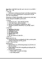
represents each detected corner is retained. Figure 1 illustrates the conventional steps of
corner detection algorithms. In this paper, we are interested in efficient corner-detector
algorithms for real-time applications. Corner strength Non-maximum computation suppression Input image Cornerness map Label map
Figure 1: Steps of corner-detector algorithms.
Rosten and Drummond [14] proposed a fast corner-detector algorithm based on ma-
chine learning. This algorithm presented good results when applied to Visual SLAM
(camera-based simultaneous localization and mapping) applications, but needed to be
combined with other algorithms to increase its robustness [9].
Sinha et al.[16] proposed a corner-detector algorithm accelerated by graphics hard-
ware (GPU). However, differently from our proposal, they used the GPU only to compute
the “image” with values of a corner response function. To suppress the non-maximum
values, the image was read back to be processed on CPU. Although their approach repre-
sented a speed-up if compared to the CPU-only counterpart, the gain in performance was
not enough for being used in Visual SLAM.
In this paper, we propose an algorithm that is fully implemented on GPU. As a result,
our algorithm is able to detect image corners very efficiently, thus being a useful tool for
real-time computer-vision applications. 3
A parallel algorithm for non-maximum suppression
The computation of an image with corresponding cornerness values associated to the
pixels, the cornerness map, can be directly mapped to the GPU parallel model. Once
we have the cornerness map, we need to select the pixel with locally maximum values,
considering a given neighborhood. First, pixels that exceed a given threshold value are
retained. This simple procedure reduces the amount of selected pixels, but does not suffice
to ensure locally maximums. In order to keep only one pixel per image corner, we have
to eliminate previously selected pixels that are within the vicinity of another pixel with
greater cornerness value. An approach to perform such an operation on CPU is described
by Tomasi and Kanade [18]: the selected pixels are sorted in decreasing order; the pixels
are then picked from the top of the list; each pixel is included in the final solution if
it does not overlap, within a given neighborhood, with any other pixel already in the
solution. Although this is a simple procedure to be implemented on CPU, it cannot be
directly mapped to GPU. Therefore, we propose a new parallel algorithm to retain only
pixels with locally maximum values. 3.1 Proposed algorithm
The algorithms input is a cornerness map where a value equal to zero means that the pixel
does not correspond to an image corner. The greater the value, the higher the probability
of the pixel being a corner. The algorithms output is another image, named label map,
where each pixel is labeled as “inside” or “outside”; the pixels labeled as “inside” belong
to the final solution, i.e. represent the position of image corners. During the course
of the algorithm, pixels are also labeled as “undefined”. In the initialization phase, the
pixels with values equal to zero are labeled as “outside”, and the others are labeled as “undefined”.
The algorithm works in multiple passes. At each pass, all pixels of the image are
conceptually processed in parallel, generating an updated label map. The end of each
pass represents a synchronization point, and the output of one pass is used as the input of
the next pass, together with the cornerness map, to produce a new updated label map. The
algorithm thus makes use of two label maps, one for input and another for output. After
each pass, the maps are swapped: the output becomes the input and the input becomes
the output for the next pass. In the GPU pixel-based parallel computational model, the
process associated to each pixel has access to any other pixel from the input map, but can
only write to the corresponding pixel in the output map. In other words, gather (indirect
read from memory) is supported but scatter (indirect write to memory) is not.
At each pass, the process associated to each pixel accesses corresponding cornerness
values, from the cornerness map, and previous labels, from the input label map. If the
pixel was previously labeled as “inside” or “outside”, the same label is simply copied to
the output map. If it is labeled as “undefined”, we need to check all the pixels in the
neighborhood of the current one. If there exists any other pixel in the neighborhood that
is already in the final solution (i.e. labeled as “inside”), the current pixel is discarded
from the solution, being labeled as “outside”. If no other pixel in the vicinity is labeled
as “inside” and the current pixel has the maximum cornerness value among all visited
pixels, the current pixel is labeled as “inside”. Note that even if there is a pixel in the
neighborhood with cornerness value greater than the current pixel, we cannot discard
this pixel, because the pixel with greater value may be discarded by another pixel just
included in the final solution. As two or more pixels may have the same cornerness value,
we have adopted a criterion to disambiguate the order in which the pixels are inserted in
the final solution. In the current implementation, we use the pixels x position and then its
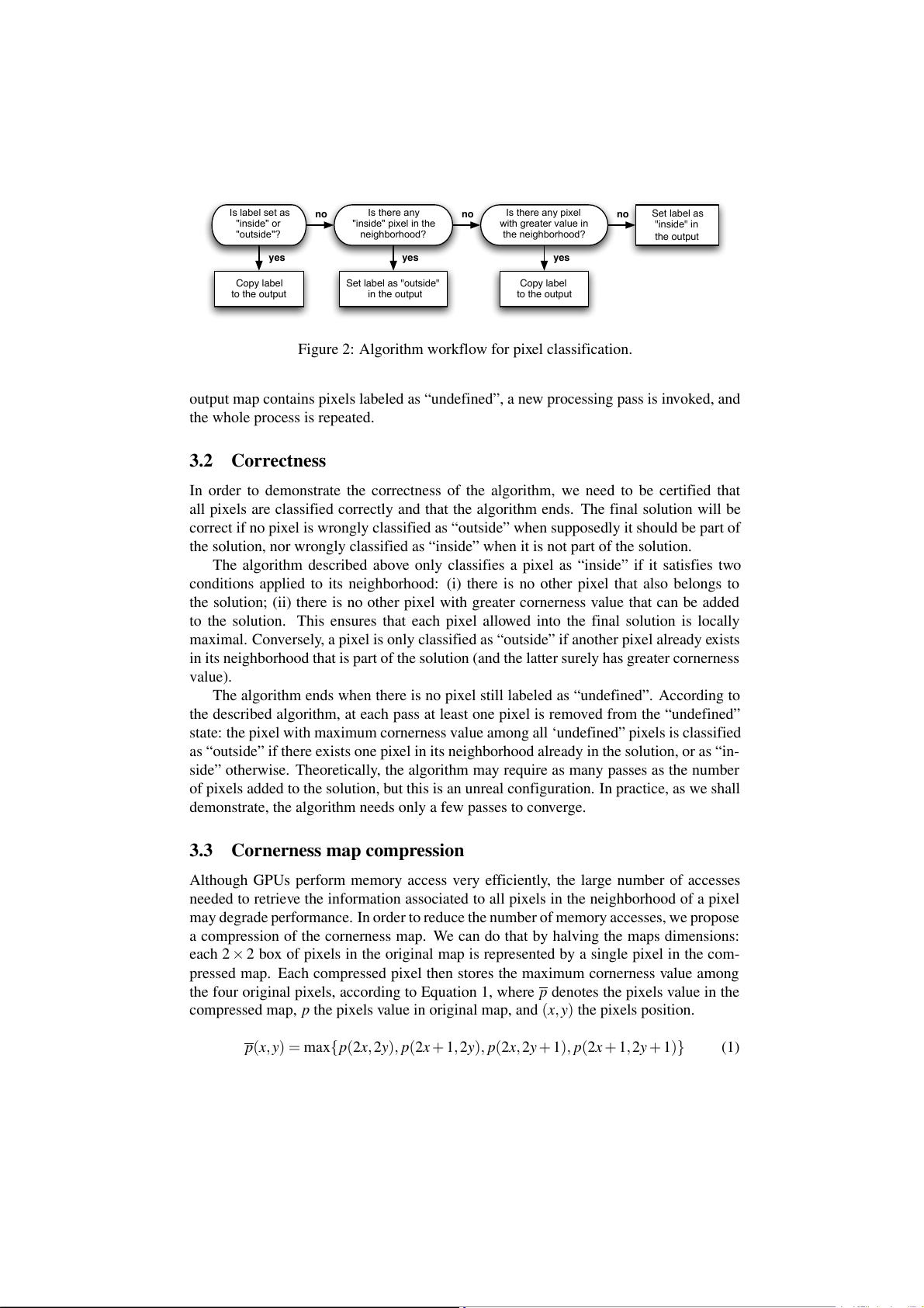
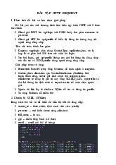
y position. The algorithm workflow for pixel classification is illustrated in Figure 2. If the Is label set as no Is there any no Is there any pixel no Set label as "inside" or "inside" pixel in the with greater value in "inside" in "outside"? neighborhood? the neighborhood? the output yes yes yes Copy label Set label as "outside" Copy label to the output in the output to the output
Figure 2: Algorithm workflow for pixel classification.
output map contains pixels labeled as “undefined”, a new processing pass is invoked, and the whole process is repeated. 3.2 Correctness
In order to demonstrate the correctness of the algorithm, we need to be certified that
all pixels are classified correctly and that the algorithm ends. The final solution will be
correct if no pixel is wrongly classified as “outside” when supposedly it should be part of
the solution, nor wrongly classified as “inside” when it is not part of the solution.
The algorithm described above only classifies a pixel as “inside” if it satisfies two
conditions applied to its neighborhood: (i) there is no other pixel that also belongs to
the solution; (ii) there is no other pixel with greater cornerness value that can be added
to the solution. This ensures that each pixel allowed into the final solution is locally
maximal. Conversely, a pixel is only classified as “outside” if another pixel already exists
in its neighborhood that is part of the solution (and the latter surely has greater cornerness value).
The algorithm ends when there is no pixel still labeled as “undefined”. According to
the described algorithm, at each pass at least one pixel is removed from the “undefined”
state: the pixel with maximum cornerness value among all ‘undefined” pixels is classified
as “outside” if there exists one pixel in its neighborhood already in the solution, or as “in-
side” otherwise. Theoretically, the algorithm may require as many passes as the number
of pixels added to the solution, but this is an unreal configuration. In practice, as we shall
demonstrate, the algorithm needs only a few passes to converge. 3.3 Cornerness map compression
Although GPUs perform memory access very efficiently, the large number of accesses
needed to retrieve the information associated to all pixels in the neighborhood of a pixel
may degrade performance. In order to reduce the number of memory accesses, we propose
a compression of the cornerness map. We can do that by halving the maps dimensions:
each 2 × 2 box of pixels in the original map is represented by a single pixel in the com-
pressed map. Each compressed pixel then stores the maximum cornerness value among
the four original pixels, according to Equation 1, where p denotes the pixels value in the
compressed map, p the pixels value in original map, and (x, y) the pixels position.
p(x, y) = max{p(2x, 2y), p(2x + 1, 2y), p(2x, 2y + 1), p(2x + 1, 2y + 1)} (1)
Together with each cornerness value in the compression map, we also store a flag
to indicate which pixel, in the 2 × 2 box of the original map, had the maximum value
and therefore was selected as the representative pixel in the compressed map. This is
important for retrieving the correct pixel position in the original image once the pixel
is inserted in the final solution. This compression results in a significant performance
gain because it reduces the neighborhood computation by a factor of four. However, it
introduces an imprecision of one pixel in the definition of the neighborhood limits. 3.4 Label map compression
One common bottleneck in GPU-based image processing algorithms consists of transfer-
ring the final resulting image back to the CPU. In order to drastically alleviate this transfer
cost, we propose compressing the label map. In the non-maximum suppression step, the
algorithm considers a rectangular neighborhood of dimension ∆ × ∆, where ∆ is an odd
number, in order to position the pixel at the center of the neighborhood region. As a con-
sequence, in the final solution, it is guaranteed that in any f × f region of pixels there is
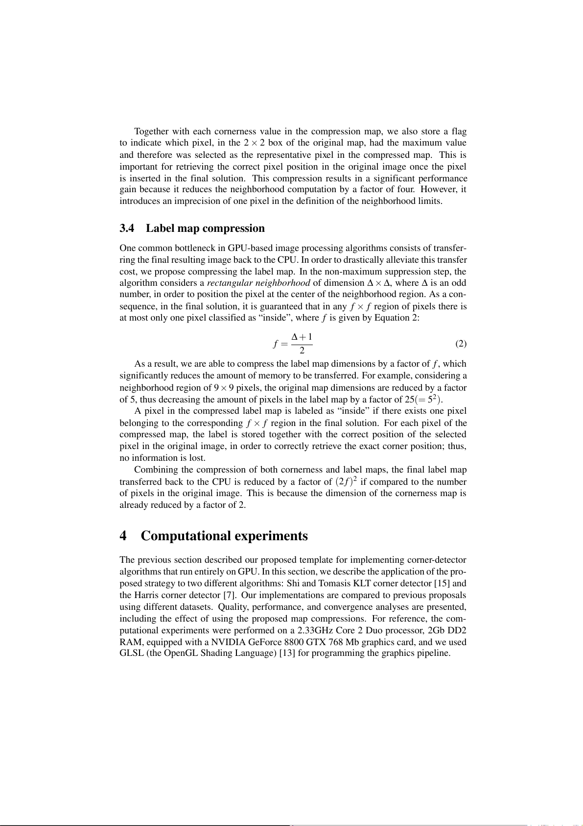
at most only one pixel classified as “inside”, where f is given by Equation 2: ∆ + 1 f = (2) 2
As a result, we are able to compress the label map dimensions by a factor of f , which
significantly reduces the amount of memory to be transferred. For example, considering a
neighborhood region of 9 × 9 pixels, the original map dimensions are reduced by a factor
of 5, thus decreasing the amount of pixels in the label map by a factor of 25(= 52).
A pixel in the compressed label map is labeled as “inside” if there exists one pixel
belonging to the corresponding f × f region in the final solution. For each pixel of the
compressed map, the label is stored together with the correct position of the selected
pixel in the original image, in order to correctly retrieve the exact corner position; thus, no information is lost.
Combining the compression of both cornerness and label maps, the final label map
transferred back to the CPU is reduced by a factor of (2 f )2 if compared to the number
of pixels in the original image. This is because the dimension of the cornerness map is
already reduced by a factor of 2. 4 Computational experiments
The previous section described our proposed template for implementing corner-detector
algorithms that run entirely on GPU. In this section, we describe the application of the pro-
posed strategy to two different algorithms: Shi and Tomasis KLT corner detector [15] and
the Harris corner detector [7]. Our implementations are compared to previous proposals
using different datasets. Quality, performance, and convergence analyses are presented,
including the effect of using the proposed map compressions. For reference, the com-
putational experiments were performed on a 2.33GHz Core 2 Duo processor, 2Gb DD2
RAM, equipped with a NVIDIA GeForce 8800 GTX 768 Mb graphics card, and we used
GLSL (the OpenGL Shading Language) [13] for programming the graphics pipeline. 4.1 Datasets and implementations
The computational experiments were executed on three different datasets that are publicly
available: (i) Oxford House: a set of 10 images with resolution of 768 × 576 pixels [3],
illustrated in Figure 3(a). For some experiments, this dataset was resized to other resolu-
tions; (ii) Oxford Corridor: a set of 10 images with resolution of 512 × 512 pixels [3],
illustrated in Figure 3(b); (iii) Alberta Floor3: a set of 500 images with resolution of
640 × 480, captured by manually driving an iRobot Magellan Pro robot around a corri-
dor [8, 10], illustrated in Figure 3(c).
For comparison, we ran the experiments using five different implementations of corner-
detector algorithms. The first two implementations, as listed below, correspond to known
third-party implementations. The third implementation was done by the authors follow-
ing the strategy described by Sinha et al. [16]. The last two implementations are fully
GPU-based according to our proposal.
• OpenCV-KLT: a CPU-based optimized implementation of the KLT tracker
available in the OpenCV Intel library [2].
• Birchfield-KLT: a CPU-based popular implementation of the KLT tracker by Birchfield [4].
• HALF GPU-KLT: our implementation of KLT tracker as suggested by Sinha et
al. [16]. In this implementation the cornerness map is computed on GPU, but the
non-maximum suppression is done using the KLT library by Sinha et al. [16].
• GPU-KLT: our full-GPU implementation of the KLT tracker in accordance with
the algorithm proposed by Birchfield [4]. The non-maximum suppression follows our proposed algorithm.
• GPU-HARRIS: our full-GPU implementation of the Harris corner detector. The
cornerness map is computed in accordance with Kovesi’s code [11], using a 3 × 3
Prewitt filter to compute the gradient. The non-maximum suppression follows our proposed algorithm.
In the last two listed implementations, the original image is sent to the GPU, which
returns the corresponding computed label map, which can then be processed on the CPU (a) Oxford House (b) Oxford Corridor (c) Alberta Floor3
Figure 3: Datasets used in the computational experiments.
to collect the selected pixels in an array. The dimension of the neighborhood area to com-
pute locally maximum values can vary in the implementations. The GPU-KLT and the
GPU-HARRIS implementations present four different variations each: with no compres-
sion, with cornerness map compression (CMC), with label map compression (LMC), and
with both cornerness map and label map compressions (CMC+LMC). 4.2 Quality evaluation
In this section, we compare our GPU-based implementations with corresponding CPU-
based counterparts. First, we compare different implementations of the KLT tracker with
the Birchfield-KLT implementation. In order to evaluate and compare the implementa-
tions, we use the metrics proposed by Klippenstein and Zhang [10]. They proposed plot-
ting recall/1 − precision curves to evaluate the detectors. The value of recall measures
the number of correct matches out of the total number of possible matches, and the value
of precision measures the number of incorrect matches out of all matches returned by the
algorithms. A perfect detector would produce a vertical line.
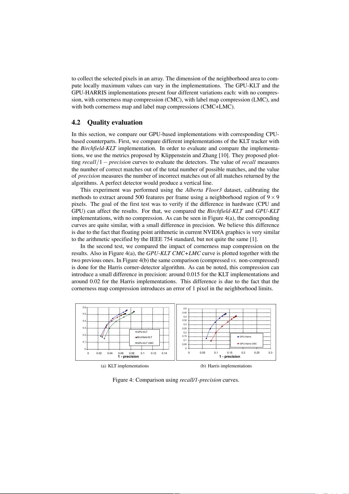
This experiment was performed using the Alberta Floor3 dataset, calibrating the
methods to extract around 500 features per frame using a neighborhood region of 9 × 9
pixels. The goal of the first test was to verify if the difference in hardware (CPU and
GPU) can affect the results. For that, we compared the Birchfield-KLT and GPU-KLT
implementations, with no compression. As can be seen in Figure 4(a), the corresponding
curves are quite similar, with a small difference in precision. We believe this difference
is due to the fact that floating point arithmetic in current NVIDIA graphics is very similar
to the arithmetic specified by the IEEE 754 standard, but not quite the same [1].
In the second test, we compared the impact of cornerness map compression on the
results. Also in Figure 4(a), the GPU-KLT CMC+LMC curve is plotted together with the
two previous ones. In Figure 4(b) the same comparison (compressed vs. non-compressed)
is done for the Harris corner-detector algorithm. As can be noted, this compression can
introduce a small difference in precision: around 0.015 for the KLT implementations and
around 0.02 for the Harris implementations. This difference is due to the fact that the
cornerness map compression introduces an error of 1 pixel in the neighborhood limits. 0.6 0.5 0.45 0.5 0.4 0.4 0.35 ll 0.3 a ll a 0.3 c 0.25 c re GPU-KLT re 0.2 0.2 0.15 Birchfield-KLT GPU-Harris 0.1 0.1 GPU-KLT CMC 0.05 GPU-Harris CMC 0 0 0 0.02 0.04 0.06 0.08 0.1 0.12 0.14 0 0.05 0.1 0.15 0.2 0.25 0.3 1 - precision 1 - precision (a) KLT implementations (b) Harris implementations
Figure 4: Comparison using recall/1-precision curves. 4.3 Convergence rate
The main goal of this work is to use GPUs for achieving real-time corner-detector algo-
rithms. Therefore, improving performance is of crucial importance for demonstrating the
effectiveness of our proposal. As we are dealing with a multiple-pass algorithm, we have
first to check how fast the algorithm converges to the final solution. As described, the
algorithm does converge to the final solution but, theoretically, this convergence may be
too slow (classifying only one pixel per pass). To verify this, we tested the algorithm’s
convergence with the three considered datasets.
The test was performed by applying the GPU-HARRIS CMC+LMC algorithm (Harris
with both map compressions). We set the neighborhood region to 9 × 9 pixels, extracting
an average number of 500 features per frame. In order to check the algorithms conver-
gence, we computed the number of detected features per pass. For all three datasets, the
first pass sufficed to detect more than 70% of the total number of features; after three
passes, the algorithm had already detected more than 90% of them. This result demon-
strates that the algorithm converges very quickly and suggests that, for real-time appli-
cations, one can drastically limit the number of passes, being aware that not all features
may be in the final solution, but the majority and most significant of them will. In order
to iterate until full convergence is reached, we use occlusion query: the process is stopped
when no pixel is added to the final solution in the last iteration. 4.4 Compression effectiveness
As shown, the cornerness map compression introduces a small precision error in feature
detection because, to compute of locally maximum values, the neighborhood limits vary
by +1 pixel. In order to check the effectiveness of both map compressions, we tested
the GPU-HARRIS considering all its variations – with and without compressions – using
different neighborhood sizes. The Oxford House dataset, reduced to a resolution of 640 ×
480, was used in this test, and an average number of 500 features were extracted per frame.
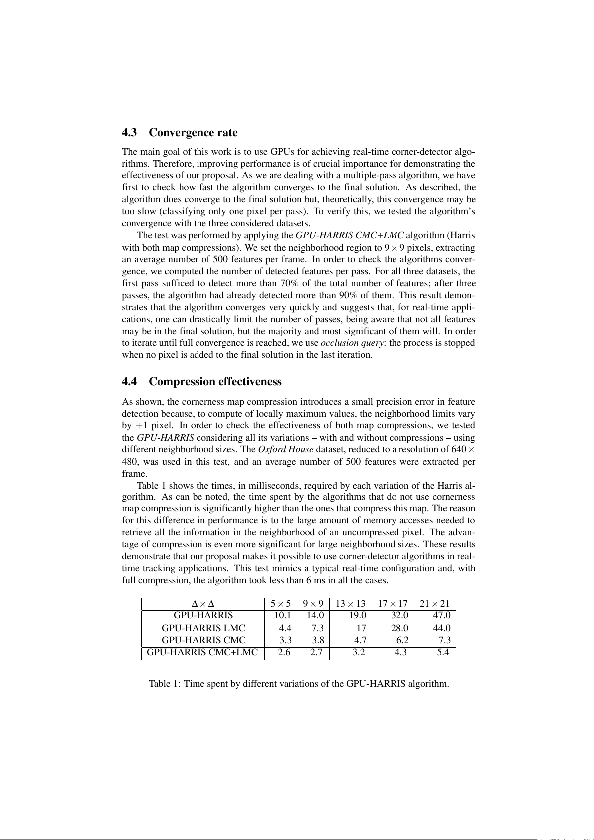
Table 1 shows the times, in milliseconds, required by each variation of the Harris al-
gorithm. As can be noted, the time spent by the algorithms that do not use cornerness
map compression is significantly higher than the ones that compress this map. The reason
for this difference in performance is to the large amount of memory accesses needed to
retrieve all the information in the neighborhood of an uncompressed pixel. The advan-
tage of compression is even more significant for large neighborhood sizes. These results
demonstrate that our proposal makes it possible to use corner-detector algorithms in real-
time tracking applications. This test mimics a typical real-time configuration and, with
full compression, the algorithm took less than 6 ms in all the cases. ∆ × ∆ 5 × 5 9 × 9 13 × 13 17 × 17 21 × 21 GPU-HARRIS 10.1 14.0 19.0 32.0 47.0 GPU-HARRIS LMC 4.4 7.3 17 28.0 44.0 GPU-HARRIS CMC 3.3 3.8 4.7 6.2 7.3 GPU-HARRIS CMC+LMC 2.6 2.7 3.2 4.3 5.4
Table 1: Time spent by different variations of the GPU-HARRIS algorithm. 4.5 Overall performance
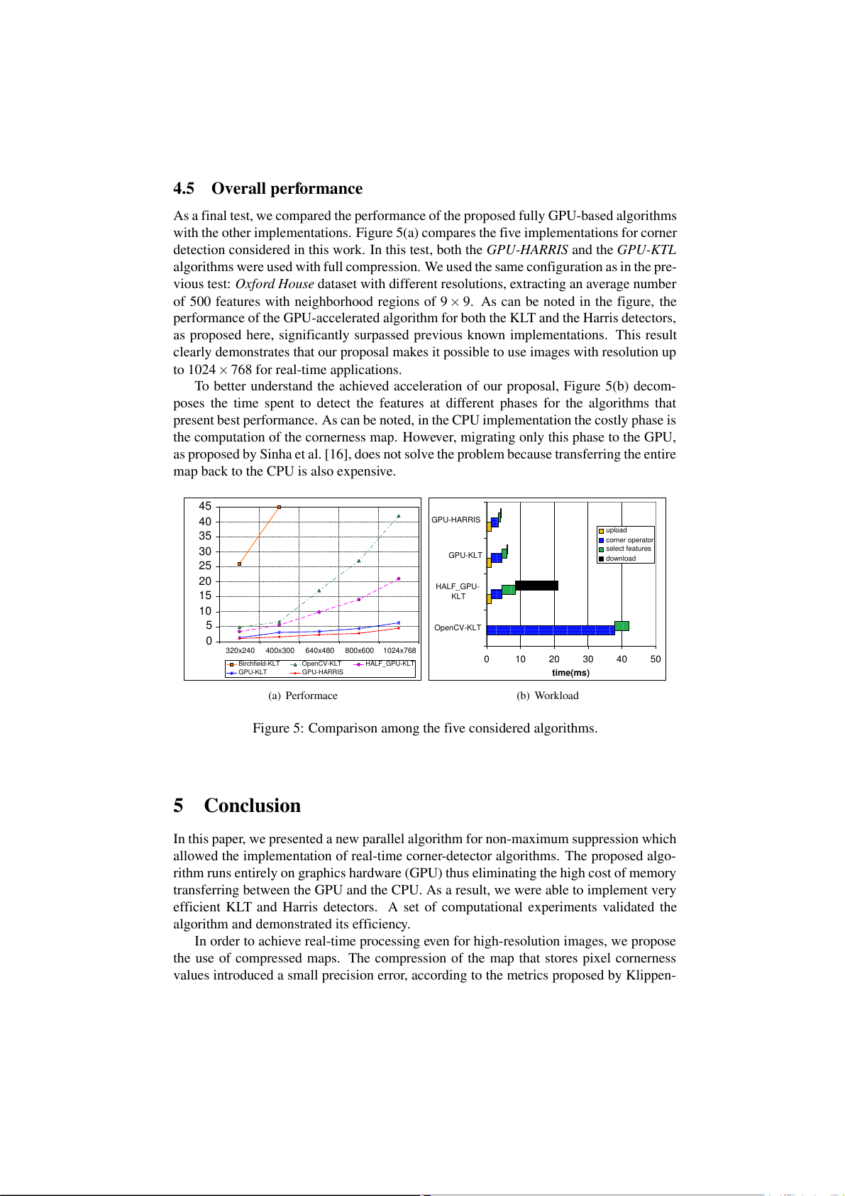
As a final test, we compared the performance of the proposed fully GPU-based algorithms
with the other implementations. Figure 5(a) compares the five implementations for corner
detection considered in this work. In this test, both the GPU-HARRIS and the GPU-KTL
algorithms were used with full compression. We used the same configuration as in the pre-
vious test: Oxford House dataset with different resolutions, extracting an average number
of 500 features with neighborhood regions of 9 × 9. As can be noted in the figure, the
performance of the GPU-accelerated algorithm for both the KLT and the Harris detectors,
as proposed here, significantly surpassed previous known implementations. This result
clearly demonstrates that our proposal makes it possible to use images with resolution up
to 1024 × 768 for real-time applications.
To better understand the achieved acceleration of our proposal, Figure 5(b) decom-
poses the time spent to detect the features at different phases for the algorithms that
present best performance. As can be noted, in the CPU implementation the costly phase is
the computation of the cornerness map. However, migrating only this phase to the GPU,
as proposed by Sinha et al. [16], does not solve the problem because transferring the entire
map back to the CPU is also expensive. 45 40 GPU-HARRIS upload 35 corner operator 30 select features ) GPU-KLT s download 25 (m e 20 tim HALF_GPU- 15 KLT 10 5 OpenCV-KLT 0 320x240 400x300 640x480 800x600 1024x768 0 10 20 30 40 50 Birchfield-KLT OpenCV-KLT HALF_GPU-KLT GPU-KLT GPU-HARRIS time(ms) (a) Performace (b) Workload
Figure 5: Comparison among the five considered algorithms. 5 Conclusion
In this paper, we presented a new parallel algorithm for non-maximum suppression which
allowed the implementation of real-time corner-detector algorithms. The proposed algo-
rithm runs entirely on graphics hardware (GPU) thus eliminating the high cost of memory
transferring between the GPU and the CPU. As a result, we were able to implement very
efficient KLT and Harris detectors. A set of computational experiments validated the
algorithm and demonstrated its efficiency.
In order to achieve real-time processing even for high-resolution images, we propose
the use of compressed maps. The compression of the map that stores pixel cornerness
values introduced a small precision error, according to the metrics proposed by Klippen-
stein and Zhang [10]. Nonetheless, map compressions resulted in a significant gain in performance.
We are currently investigating alternative methods for non-lossy cornerness map com-
pressions. One idea is to use the color channels to store all the four values of a 2x2 region.
This will probably impact performance due to the SIMD (single instruction, multiple data)
architecture of graphics processors. Further studies have to be carried out in order to better evaluate the benefits.
Acknowledgement. We thank the Oxford Visual Geometry Group for providing ac-
cess to the Oxford datasets [3]. The Alberta dataset was obtained from the Robotics Data
Set Repository (Radish) [8]; thanks go to J. Klippenstein for providing this data. References
[1] GPGPU: General-purpose computation using graphics hardware. www.gpgpu.org.
[2] Intel OpenCV: Open source computer vision library. www.intel.com/research/mrl/ research/opencv/.
[3] Oxford datasets. www.robots.ox.ac.uk/ vgg/data/. ~
[4] S. Birchfield. KLT: An implementation of the Kanade-Lucas-Tomasi feature tracker. www.
ces.clemson.edu/stb/klt/, 2007.
[5] A. Davison. Real-time simultaneous localisation and mapping with a single camera. In Proc.
International Conference on Computer Vision,Nice, 2003.
[6] O. Fialka and M. Cadik. FFT and convolution performance in image filtering on gpu. Tenth
Int. Conf. on Information Visualization, pages 609–614, July 2006.
[7] C. Harris and M. Stephens. A combined corner and edge detector. In Proceedings of The
Fourth Alvey Vision Conference, pages 147–152, 1988.
[8] Andrew Howard and Nicholas Roy. The robotics data set repository (Radish), 2003.
[9] Georg Klein and David Murray. Parallel tracking and mapping for small AR workspaces. In
Proc. Sixth IEEE and ACM International Symposium on Mixed and Augmented Reality, 2007.
[10] J. Klippenstein and H. Zhang. Quantitative evaluation of feature extractors for visual slam. In
Proceedings of the Fourth Canadian Conference on Computer and Robot Vision, 2007.
[11] P. Kovesi. MATLAB and Octave functions for computer vision and image processing. The
University of Western Australia. www.csse.uwa.edu.au/ pk/research/matlabfns. ~
[12] H. Moravec. Obstacle avoidance and navigation in the real world by a seeing robot rover. In
tech. report CMU-RI-TR-80-03, Robotics Institute, Carnegie Mellon University. 1980.
[13] R. Rost. OpenGL Shading Language. Addison-Wesley, 2004.
[14] E. Rosten and T. Drummond. Machine learning for high-speed corner detection. In European
Conference on Computer Vision, volume 1, pages 430–443, May 2006.
[15] J. Shi and C. Tomasi. Good features to track. In IEEE Conference on Computer Vision and
Pattern Recognition (CVPR’94), Seattle, June 1994.
[16] S. Sinha, J. Frahm, M. Pollefeys, and Y. Genc. Feature tracking and matching in video using
programmable graphics hardware. Machine Vision and Applications, 2007.
[17] S. Smith and J. Brady. SUSAN – A new approach to low level image processing. Technical
Report TR95SMS1c, Chertsey, Surrey, UK, 1995.
[18] C. Tomasi and Kanade T. Detection and tracking of point features. Technical Report CMU-
CS-91-132, Carnegie Mellon University, 1991.
[19] M. Trajkovic and M. Hedley. Fast corner detection. Image and Vision Computing, 16, 1998. View publication stats
Tài liệu liên quan:
-
Đồ án tốt nghiệp Công nghệ thực tế ảo và ứng dụng | Học viên Công Nghệ Bưu Chính Viễn Thông
11 6 -
Tóm tắt lý thuyết môn IoT và ứng dụng | Học viện Công Nghệ Bưu Chính Viễn Thông
49 25 -
Đề xuất Dự án IoT: Thiết bị phát hiện chạm cho xe máy | Iot và ứng dụng | Học viện Công nghệ Bưu chính Viễn thông
57 29 -
Phân Tích và Giải Pháp FastAPI | Iot và ứng dụng | Học viện Công nghệ Bưu chính Viễn thông
51 26