Assignment on Naive Bayes and K-Means for Covid-19 Analysis | Môn Mạng máy tính nâng cao - Đại học Xây Dựng Hà Nội

lOMoAR cPSD| 58970315 64CS
Naive Bayes and K-means Covid-19 2th year A – Naïve Bayes 1 Assignment 1.1 Intro
Handwriting recognition is the ability of a computer to interpret hand written text as the characters.In this
assignment we will be trying to recognize numbers from images. To accomplish this task, we will be using a Naive Bayes classifier.
Naive Bayes classifiers are a family of probabilistic classifiers that are based on Bayes’ theorem.These
algorithms work by combining the probabilities that an instance belongs to a class based on the value of a
set of features. In this case we will be testing if images belong to the class of the digits 0 to 9 based on the
state of the pixels in the images. 1.2 Provided Files
We are providing data files representing handwriting images along with the correct classification of these
images. These are provided as a zip file that you can find at the following URL.
https://ndquy.github.io/assets/docs/digitdata.zip This
zip file contains the following.
¥ readme.txt - description of the files in the zip
¥ testimages - 1000 images to test
¥ testlabels - the correct class for each test image
¥ trainingimages - 5000 images for training
¥ traininglabels - the correct class for each training image
We will be using the training images to train our classifier specifically to compute probabilities that we will
use and then try to recognize the test images. You should use the .gitignore file to prevent these files from
being added to your git repository. 1.3 Image Data Description
The image data for this consist of 28x28 pixel images stored as text. Each image has 28 lines of text with
each line containing 28 characters. The values of the pixels are encoded as ’ ’ for white and ‘+‘ for gray and
finally ’#’ for black. You can view the images by simply looking at them with a fixed width font in a text
editor. We will be classifying images of the digits 0-9, meaning that given a picture of a number we should
be able to accurately label which number it is.
Since computers can’t tell what a picture is we’re going to have to describe the input data to it in a way
that it can understand. We do this by taking an input image and extracting a set of features from it. A
feature simply describes something about our data. In the case of our images we can simply break the
image up into the grid formed by its pixels and say each pixel has a feature that describes its value.
We will be using these images as a set of binary features to be used by our classifier. Since the image is 28
x 28 pixels we will have 28 x 28 = 784 features for each input image. To produce binary features from this
data we will treat pixel i, j as a feature and say that Fi,j has a value of 0 if it is a background pixel - white,
and 1 if foreground - grey or black. In this case we are generalizing the two foreground values of gray and
black as the same to simplify our task. lOMoAR cPSD| 58970315 64CS
Naive Bayes and K-means Covid-19 2th year 2 Naive Bayes Algorithm 2.1 Overview
Naive Bayes classifiers are based on Bayes’ theorem which describes the probability of an event based on
prior knowledge of conditions that might be related to the event. In our case we are computing the
probability that an image might belong to a class based on the value of a feature. This idea is called
conditional probability and is the likelihood of event A occurring given event B and is written as P (A|B).
From this we get Bayes’ theorem.
P (A|B) = P (B|A)P (A) P (B) This
says that if A and B are events and P (B) ˜= 0 then
¥ P (A|B) is the probability that A occurs given B
¥ P (B|A) is the probability that B occurs given A
¥ P (A) the probability A occurs independently of B
¥ P (B) the probability B occurs independently of A
Applying this to our case we want to compute for each feature the probability that given the feature Fi,j
has a value !" #" $%& ’( that the image will belong to a given class c )" # $"%& ’& * & +(. To do this we
will train our model on a large set of images where we know the class that they belong to. Once we have
computed these probabilities we will be able to classify images by computing the class with the highest
probability given all the known features of the image and assign it to that class.
From this we get two phases of the algorithm.
¥ Training - compute the conditional probability that for each feature that an image is part of each class.
¥ Classifying - for each image compute the class that it is most likely to be a member of given the
assumed independent probabilities computed in the training stage. 2.2 Training
The goal of the training stage is to teach the computer the likelihoods that a feature Fi,j has value f # {0,
1} as we have binary features, given that the current image is of class c # {0, 1, ..., 9}, which we can
write as P (Fi,j = f|class = c)
This can be simply computed as follows:
Given how we will use these probabilities we need to ensure that they are not zero since if they are it will
cause them to cancel out any non-zero probability from other features. To do this we will use a technique
called Laplace Smoothing. This technique works by adding a small positive value k to the numerator above,
and k . V to the denominator (where V is the number of possible values our feature can take on so 2 in our Æ
case). The higher the value of k , the stronger the smoothing is. So for our binary features that would give us: lOMoAR cPSD| 58970315 64CS
Naive Bayes and K-means Covid-19 2th year
You can experiment with different values of k (say, from 0.1 to 10) and find the one that gives the highest classification accuracy.
You should also estimate the priors P (class = c) or the probability of each class independent of features by
the empirical frequencies of different classes in the training set.
With the training done you will have an empirically generated set of probabilities that can be referred to
as the model that we will use to do classification on unknown data. This model once generated can be
used in the future without needing to be regenerated. 2.3 Classifying
To classify the unknown images using the trained model you will perform maximum a posteriori (MAP)
classification of the test data using the trained model. This technique computes the posterior probability
of each class for the particular image. Then classifies the image as belonging to the class which has the
highest posterior probability.
Since we assume that all the probabilities are all independent of each other we can compute the
probability that the image belongs to the class by simply multiplying all the probabilities together and
dividing by the probability of the feature set. Finally, since we don’t actually need the probability but
merely to be able to compare the values we can ignore the probability of the feature set and thus compute the value as follows:
Unfortunately, when computers do floating point arithmetic they are not quite computing as we do by
hand and they can produce a type of error called underflow. More information on this can be found here:
https://en.wikipedia.org/wiki/Arithmetic_underflow
To avoid this problem, we will compute using the log of each probability rather than the actual value. This
way the actual computation will be the following:
Where fi,j is the feature value of the input data. You should be able to use the priors and probabilities you
calculated in the training stage to calculate these posterior probabilities.
Once you have a posterior probability for each class from 0-9 you should assign the test input to the class
with the highest posterior probability. For example for an input P, if we had the posterior probabilities: lOMoAR cPSD| 58970315 64CS
Naive Bayes and K-means Covid-19 2th year class posterior probability 0 .3141 1 .432 2 0 3 0 4 .4 5 .004 6 .1 7 .2 8 .7 9 .5
We’d classify P as an 8 as that is the class with the highest posterior probability. 3 Requirements
To complete this assignment you will need to use python to write a program the uses the Naive Bayes
Algorithm described above to classify the provided images. This program must run on the google colab with functions:
¥ Read training data from files and generate a model
¥ Save a model as a file
¥ Load a model from a file
¥ Classify images from a file
Remember to plan your assignment out before writing it and breaking it apart into the appropriate
necessary functions and book keeping values that you will need to keep.
Finally you will also need to evaluate your classifier. 3.1 Evaluation
Use the true class labels of the test images from the testlabels file to check the correctness of your model.
Report your confusion matrix. This is a 10 x 10 matrix whose entry in row r and column c is the percentage
of test images from class r that are classified as class c.
In the ideal case this matrix would have a 1 on the diagonal and 0 elsewhere since that would happen
when every every image was correctly identified. This will not happen with our classifier since they are not
that good. There is not a single correct answer for this section but it will help you understand the
performance of your classifier.
If you have time you can also try to following.
¥ Play around with the Laplace smoothing factor to figure out how to get the best performance out of your classifier.
¥ Try changing the order you feed in your training data, randomizing it to see if it changes the results of your classifier. 3.2 Extra Credit
¥ Perform K-cross form validation with different values of K to improve classification accuracy lOMoAR cPSD| 58970315 64CS
Naive Bayes and K-means Covid-19 2th year
¥ Use ternary features (by taking into account the two foreground values to see if classification accuracy improves
Use groups of pixels as features, perhaps 2 x 2 pixel squares where the value of a feature is the
majority value of its composing pixels lOMoAR cPSD| 58970315 64CS
Naive Bayes and K-means Covid-19 2th year 3.3 Glossary
We’re aware that you were presented with many terms and mathematical concepts so we’ve
assembled a glossary here for you to refer to.
Probability P (X) is the probability that some event X happens and is a value between 0 and 1.
Conditional probability P (A | B) is the probability that some event A happens given that B has already happened.
P (A , B) P (A|B) = P (B)
Bayes Theorem Predicts probability of an event based on knowledge we already have
P (C|X) = P (C) - P (X|C) P (X)
Feature We use features to describe a characteristic of the input data. A feature set is the set of all features
that describe a piece of input data. In our case we have 1 feature for each pixel in a 28 × 28 image so we
have 784 features Fi,j
Class Class describes the label of a piece of data. In our case our classes can take any value from 0-9
Laplace Smoothing Add some k to the numerator in ./0ị" 1 !"2)3455 1 )6 and k.V where V is the number
of values the features can take to the denominator. This ensures there are no zero counts and the posterior probability is not zero
Maximum A Posteriori MAP classification is used to classify what the label of a test input. We calculate
the posterior probabilities of all the classes and assign the class with highest posterior probability to our input.
Confusion Matrix A 10 x 10 matrix where entry (R x C) tells you what percentage of test images from class
R where classified as class C
Model A model in machine learning is the result of training on a data set. In this case the model is the set
of probabilities for each feature and class. B – K-Means 1 Assignment 1.1 Intro
Customer Segmentation can be a powerful means to identify unsatisfied customer needs. This technique
can be used by companies to outperform the competition by developing uniquely appealing products and services.
Customer Segmentation is the subdivision of a market into discrete customer groups that share similar
characteristics. Customer Segmentation can be a powerful means to identify unsatisfied customer needs. lOMoAR cPSD| 58970315 64CS
Naive Bayes and K-means Covid-19 2th year
Using the above data companies can then outperform the competition by developing uniquely appealing products and services.
The most common ways in which businesses segment their customer base are:
¥ Demographic information, such as gender, age, familial and marital status, income, education, and occupation.
¥ Geographical information, which differs depending on the scope of the company. For localized
businesses, this info might pertain to specific towns or counties. For larger companies, it might
mean a customer’s city, state, or even country of residence.
¥ Psychographics, such as social class, lifestyle, and personality traits.
¥ Behavioral data, such as spending and consumption habits, product/service usage, and desired benefits. 1.2 Provided Files
We have a supermarket mall and through membership cards , you have some basic data about your
customers like Customer ID, age, gender, annual income and spending score. The file consist of
informations from 200 customers.
To download file, you can go to the following URL:
https://ndquy.github.io/assets/docs/Mall_Customers.csv 2
K Means Clustering Algorithm
To perform k-means algorithm, do the following steps:
1. Specify number of clusters K.
2. Initialize centroids by first shuffling the dataset and then randomly selecting K data points for the
centroids without replacement.
3. Keep iterating until there is no change to the centroids. i.e assignment of data points to clusters isn’t changing. 2.1
Find the optimal number of cluster K
To find the number of cluster K, you can use WCSS value. WCSS measures sum of distances of observations
from their cluster centroids which is given by the below formula. !"## $% &’(! ) *!+%" ! ∈%
where Yi is centroid for observation Xi. The main goal is to maximize number of clusters and in limiting
case each data point becomes its own cluster centroid.
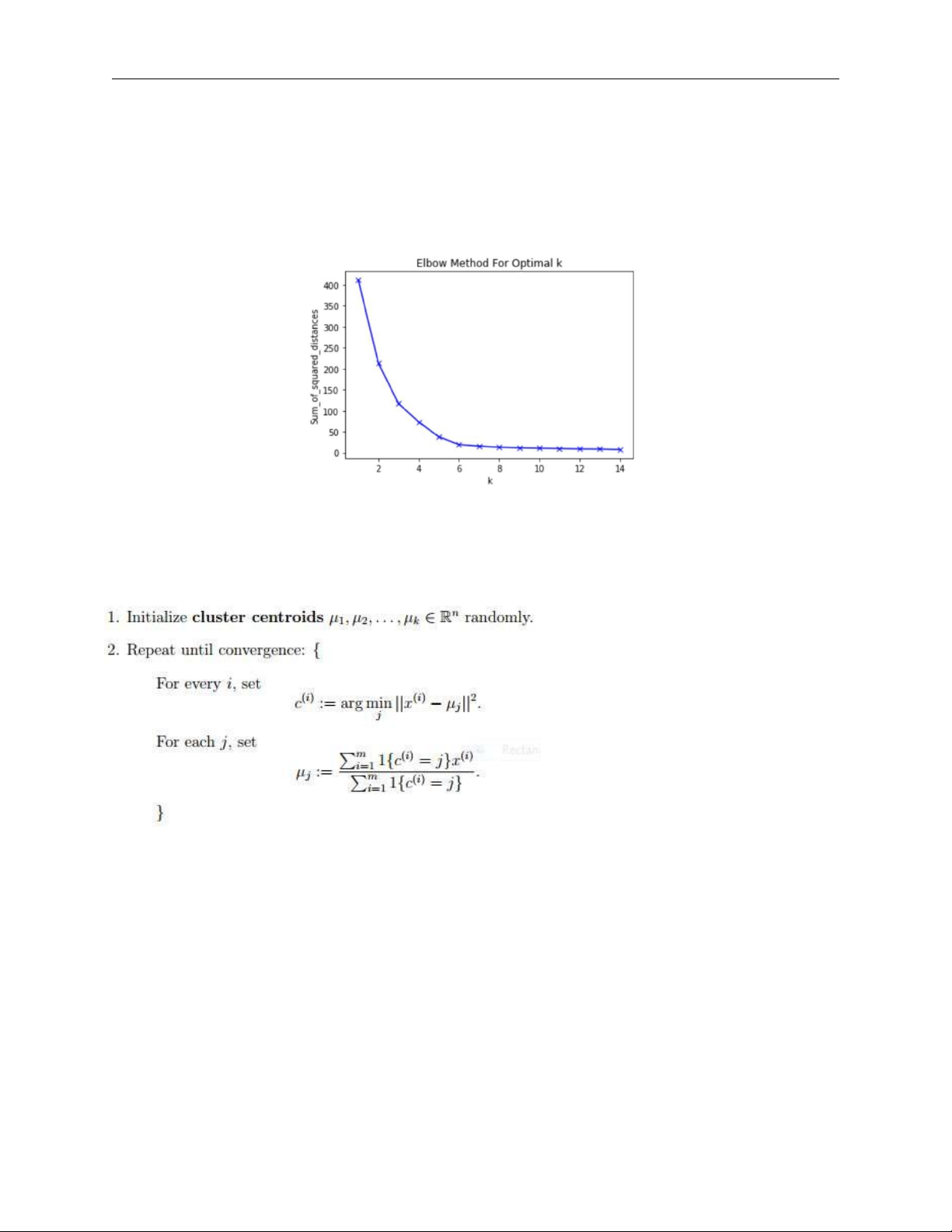
Detailly, For each k value, we will initialise k-means and use the inertia attribute to identify the sum of
squared distances of samples to the nearest cluster centre. lOMoAR cPSD| 58970315 64CS
Naive Bayes and K-means Covid-19 2th year
As k increases, the sum of squared distance tends to zero. Imagine we set k to its maximum value n (where
n is number of samples) each sample will form its own cluster meaning sum of squared distances equals zero.
Below is a plot of sum of squared distances for k in the range specified above. If the plot looks like an arm,
then the elbow on the arm is optimal k.
In the plot above the elbow is at k=5 indicating the optimal k for this dataset is 5. 2.2 The Algorithm
The k-means clustering algorithm is as follows: 3 Requirements
To complete this assignment you will need to use python to write a program the uses the k-means
algorithm described above to predict clusters the provided data. This program must run on the google colab with requirements:
1. Implement K-means using numpy only, do not use any machine learning library.
2. Find the optimal k – cluster
3. Run k-means with the optimal k.
4. Visualizing K-Means Clustering results to understand the clusters.
5. Make understanding about the data after clustering.