Audio and Audio Compression| Bài giảng môn Truyền thông đa phương tiện| Trường Đại học Bách Khoa Hà Nội

AUDIO & AUDIO COMPRESSION Dr. Quang Duc Tran Sound Facts
• Sound is a continuous wave that travels through the air. The
wave is made up of pressure differences
• Sound waves have normal wave properties (reflection, refraction, diffraction etc.)
• Frequency represents the number of periods in a second and
is measured in hertz (Hz) or cycles per second.
• Amplitude is the measure of displacement of the air pressure
wave from its means. It is related to but not the same as loudness. Digital Audio
• Audio signal that is encoded in digital form ▫ Sampling ▫ Quantization • Sampling rate ▫ Telephone: 8 kHz ▫ CD-audio: 44.1 kHz • Quantization ▫ Speech: 8 bit ▫ CD-audio: 16 bit • Number of soundtracks ▫ Stereo: 2 channels
▫ Professional: 16, 32 or more. Digital Audio (Cont.)
• Example 1: Sampling a four second sound of a speaking voice
▫ Because the voice is in the lower range of the audio
spectrum, we could sample the sound at 8 kHz with a mono channel and 8-bit resolution
• Example 2: Sampling a four second sound of a musical selection
▫ In order to capture the complex musical sound, the
sampling rate should be 44.1 kHz. We will record a
stereo sample with 16-bit resolution. Audio Compression
• Differential Pulse Code Modulation (DPCM)
• Adaptive Differential Pulse Code Modulation (ADPCM)
• Linear Predictive Coding (LPC) • Perceptual Coding • MPEG Audio Compression DPCM
• The range of differences in amplitudes between
successive samples of the audio waveform is less than
the range of the actual sample amplitudes. Hence, fewer
bits to represent the difference signals.
• Designing of DPCM is easy. Prediction is then based on
the previously coded/transmitted samples.
• Because the co-relation between successive are very
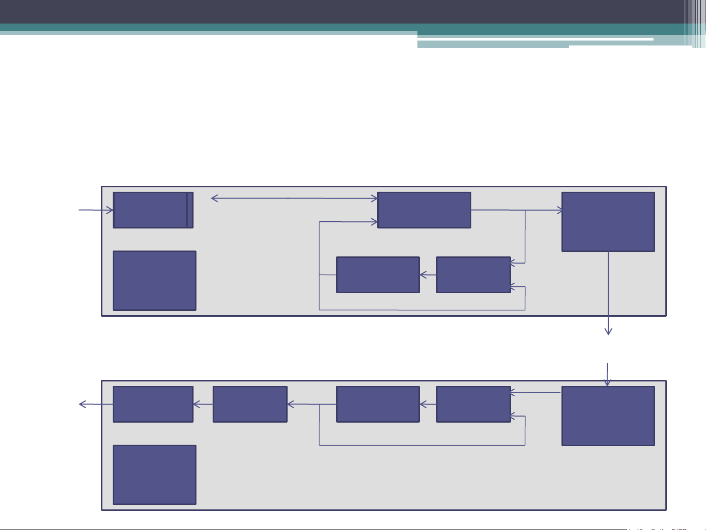
good, so the output sample is far better than that of PCM. DPCM (Cont.) Speech Input AAF ADC Subtractor Parallel- Signal to-serial converter Register Timing + Adder R Control Network Speech Register Output AAF ADC Serial-to- Adder R parallel Signal converter Timing + Control DPCM (Cont.) • Encoder
▫ Previous digitized sample is held in the register (R).
▫ The DPCM signal is computed by subtracting the current
content (R) from the new output by the ADC.
▫ The register value is then updated before transmission. • Decoder
▫ Decoder simply adds the previous register contents (PCM) with the DPCM.
▫ Since ADC will have noise there will be cumulative errors in
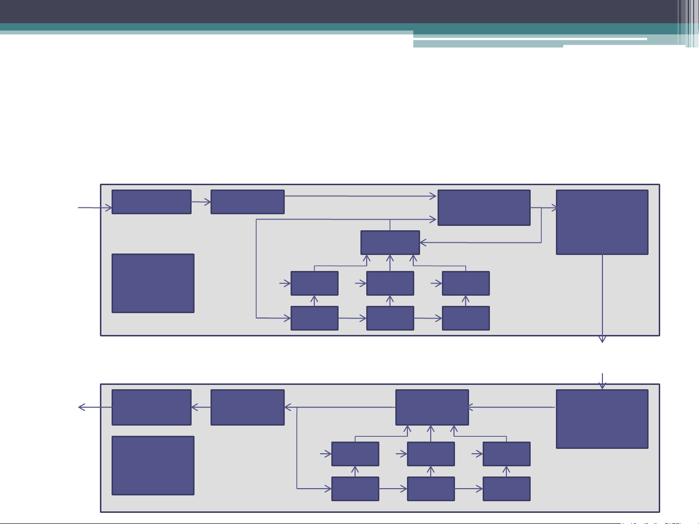
the value of the register signal. Third-order predictive DPCM Speech AAF ADC Input Subtractor Parallel- Signal to-serial converter Adder Timing + C1 x C2 x C3 x Control R1 R2 R3 Network Speech Output AAF ADC Serial-to- Adder parallel Signal converter Timing + C1 x C2 x C3 x Control R1 R2 R3
Third-order predictive DPCM (Cont.)
• To eliminate the noise effect, predictive techniques are
used to predict a more accurate version of the previous
signal (i.e., using not only the current signal but also
varying proportions of a number of the preceding estimated signals).
• These proportions used are known as predictor coefficients.
• Different signal is computed by subtracting varying
proportion of the last three predicted values from the current output by the ADC
Third-order predictive DPCM (Cont.)
• R1, R2, R3 will be subtracted from PCM.
• The values in the R1 register will be transferred to R2
and R2 to R3 and the new predicted value goes into R1.
• Decoder operates in a similar way by adding the same
proportions of the last three computed PCM signals to the received DPCM signal. Adaptive DPCM (ADPCM)
• Saving of bandwidth is possible by varying the number of bits
used for the difference signal depending on its amplitude.
• An international standard for this is defined in ITU-T Recommendation G.721.
• The principle is similar to that of DPCM except an eight-order
predictor is used and the number of bits used to quantize each difference is varied.
• Larger step-size is used to encode differences between high
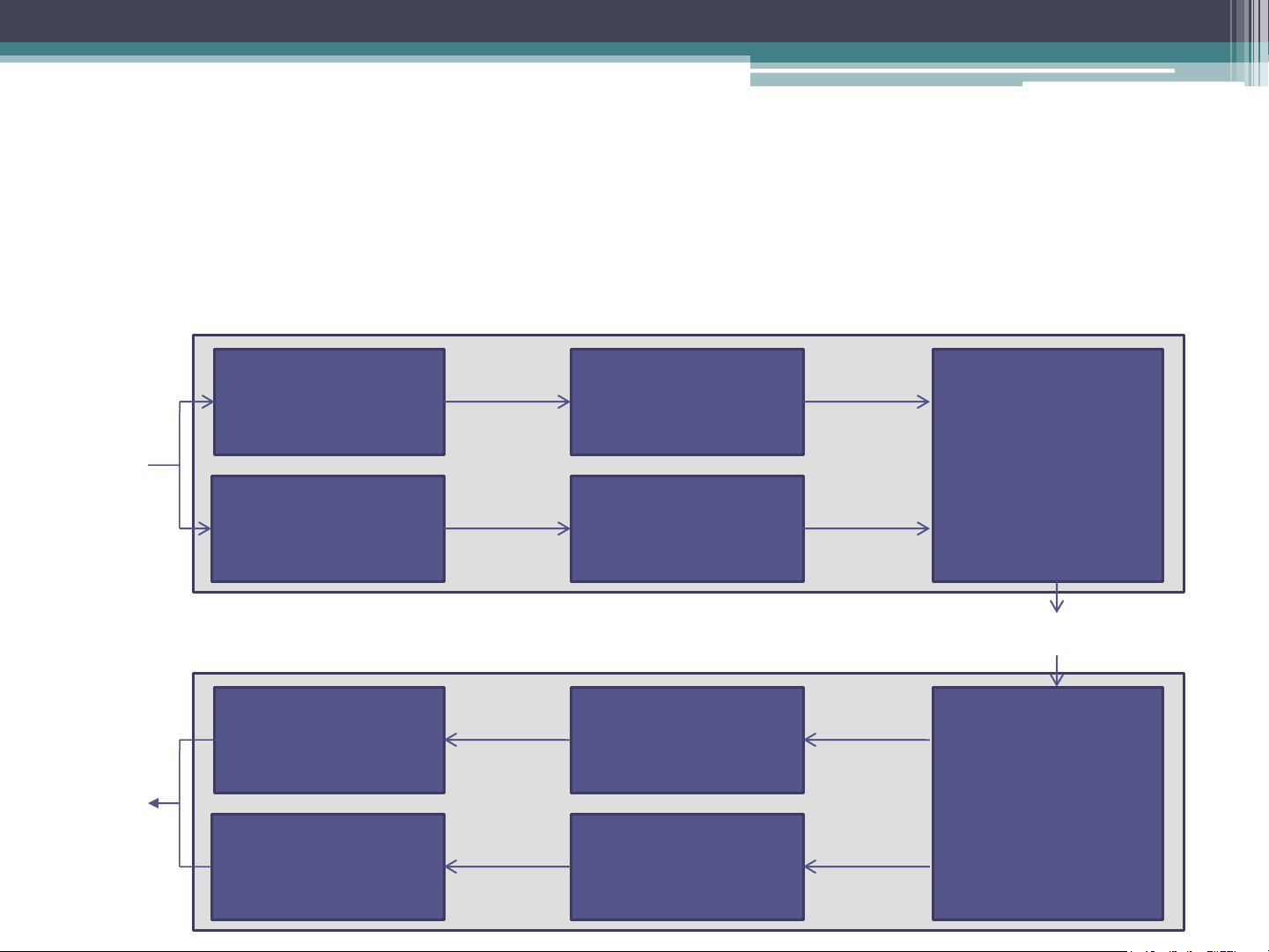
frequency samples and smaller step-size for differences between low frequency samples. Sub-band ADPCM Lower sub-band Lower sub-band 48 kbps bandlimiting filter ADPCM encoder Speech (50Hz-3.5 kHz) Input Multiplexer Signal Upper sub-band Upper sub-band 16 kbps bandlimiting filter ADPCM encoder (3.5kHz-7kHz) Network Lower sub-band Lower sub-band 48 kbps low-pass filter ADPCM decoder Speech (50Hz-3.5 kHz) Output Demultiplexer Signal Upper sub-band Upper sub-band 16 kbps low-pass filter ADPCM decoder (3.5kHz-7kHz) Sub-band ADPCM
• The sub-band ADPCM is defined in ITU-T Recommendation
G.722 (better sound quality in VoIP).
• This uses sub-band coding, in which the input signal prior to
sampling is passed through two filters: one which passes only
signal frequencies in the range 50 Hz through to 3.5 kHz and
the other only frequencies in the range 3.5 kHz through to 7 kHz.
• Each is then sampled and encoded independently using
ADPCM. 6 digits are used to encode the lower sub-band
signal, while 2 digits are used to encode the upper sub-band signal. Linear Predictive Coding
• Linear Predictive Coding derives its name from the fact that
current speech sample can be closely approximated as a linear
combination of past samples. The approximation is done on
short chucks of the speech signal, called frames. Generally, 30
to 50 frames per second give intelligible speech with good compression. Order of the model Prediction coefficient p
x[n] = a x[n − k]+ e[n] k k =1 Previous speech samples Prediction error
Linear Predictive Coding (Cont.)
• The predictor coefficients are determined by minimizing the
sum of squared differences (over a finite interval) between the
actual speech samples and the linearly predicted ones.
• The higher the coefficient order p, the closer the approximation is.
• Uncompressed speech is transmitted at 64 kbps. The LPC
transmits speech at a bit rate of 2.4 kbps. There is a noticeable
loss of quality, however, the speech is still audible.
• LPC is used by phone companies (e.g., GSM standard). Code-excited LPC (CELPC)
• In CELPC model instead of treating each digitized frame
independently for encoding purposes, just a limited set
of frames are used, each known as a wave template.
• A pre-computed set of templates are held by the encoder
and the decoder in what is known as the template codebook.
• Each of the individual digitized samples that make up a
particular template in the codebook are differently encoded. Perceptual Coding
• LPC and CELPC are used for telephony applications. PC is
designed for compression of general audio associated with
a digital television broadcast.
• Sampled frames of the source audio waveform are analyzed
– but only those features that are perceptible to the ear are transmitted.
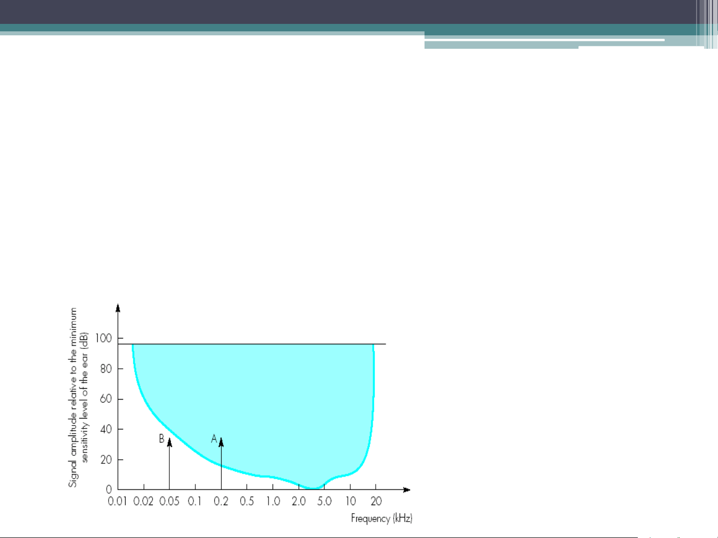
• Although the human ear is sensitive to signals in the range
15 Hz to 20 kHz, the level of sensitivity to each signal is
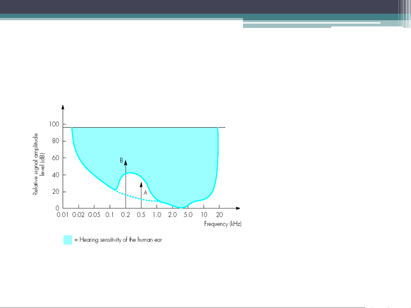
non-linear, i.e., the ear is more sensitive to some signals than others. Sensitivity of the ear
• Sensitivity of the ear varies with the frequency of the signal.
The ear is most sensitive to signals in the range 2-5 kHz
• The dynamic range of ear is defined as the loudest sound it
can hear to the quietest sound. Signal A is above the hearing threshold and B is below the hearing threshold Frequency Masking Signal B is larger than signal A. This causes the basic sensitivity curve to be distorted. Signal A will no longer be heard as it is within the distortion band.
• When multiple signals are present, a strong signal may reduce
the level of sensitivity of the ear to other signals which are near to it in frequency