Bài giảng Logistic Regression môn Phân tích thuật toán | Trường Đại học Khoa học tự nhiên, Đại học Quốc gia Thành phố Hồ Chí Minh

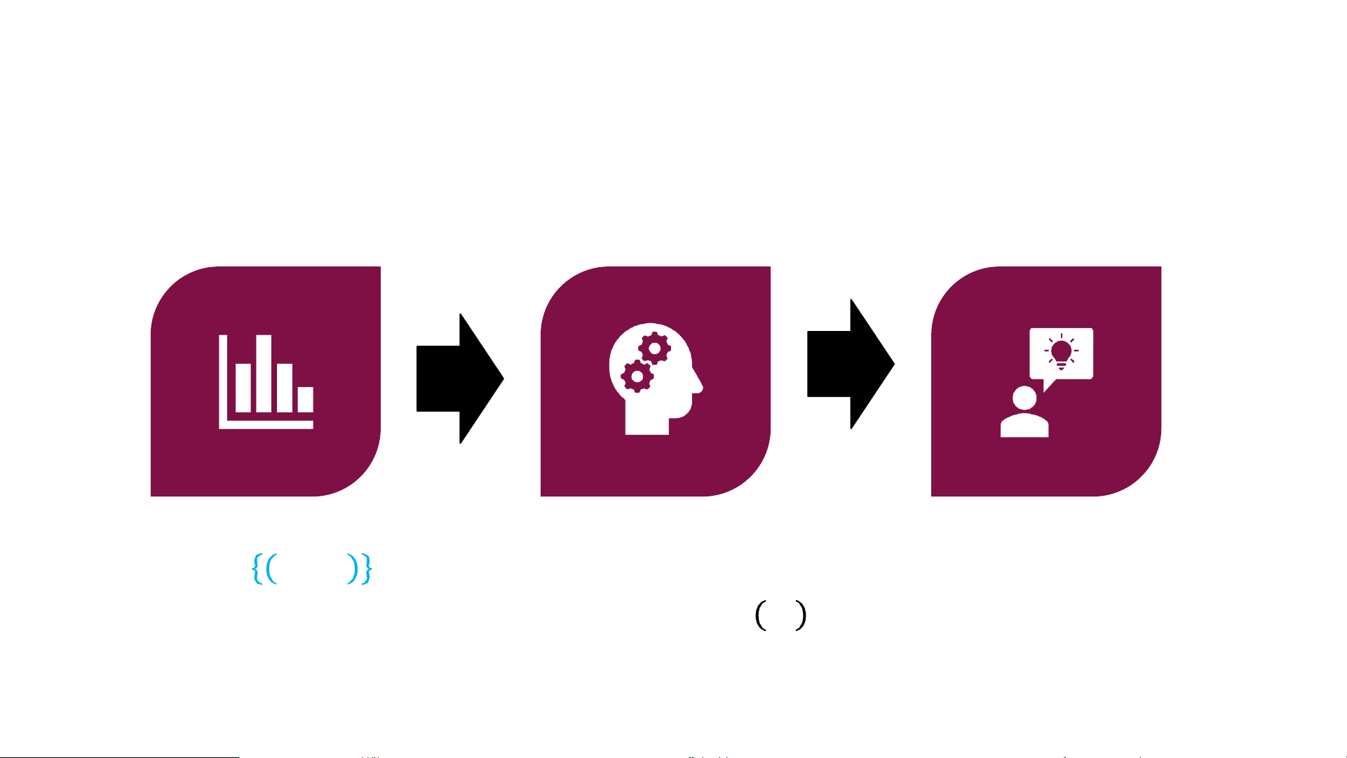
Lecture 6: Logistic Regression Instructor: Thao. Ng Dac P Major: AI&DS Outlook: ndpthao@tlu.edu.vn Supervised Learning Data 𝑍 = 𝑥 𝑛 𝑖, 𝑦𝑖 ෝ 𝜔(𝑍) = arg 𝑚𝑖𝑛 𝑖=1 𝜔𝐿(𝜔;𝑍) Model 𝑓ෝ𝜔(𝑍)
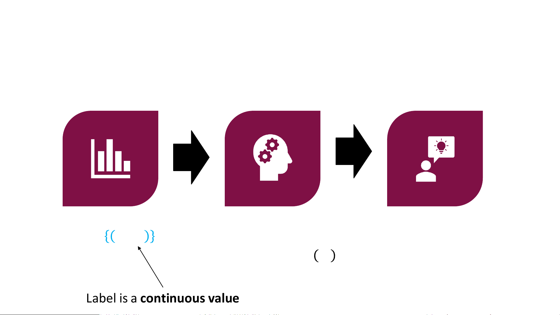
𝐿 encodes 𝑦𝑖 ≈ 𝑓𝜔 𝑥𝑖 Regression Data 𝑍 = 𝑥 𝑛 𝑖, 𝑦𝑖 ෝ 𝜔(𝑍) = arg 𝑚𝑖𝑛 𝑖=1 𝜔𝐿(𝜔;𝑍) Model 𝑓ෝ𝜔(𝑍)
𝐿 encodes 𝑦𝑖 ≈ 𝑓𝜔 𝑥𝑖
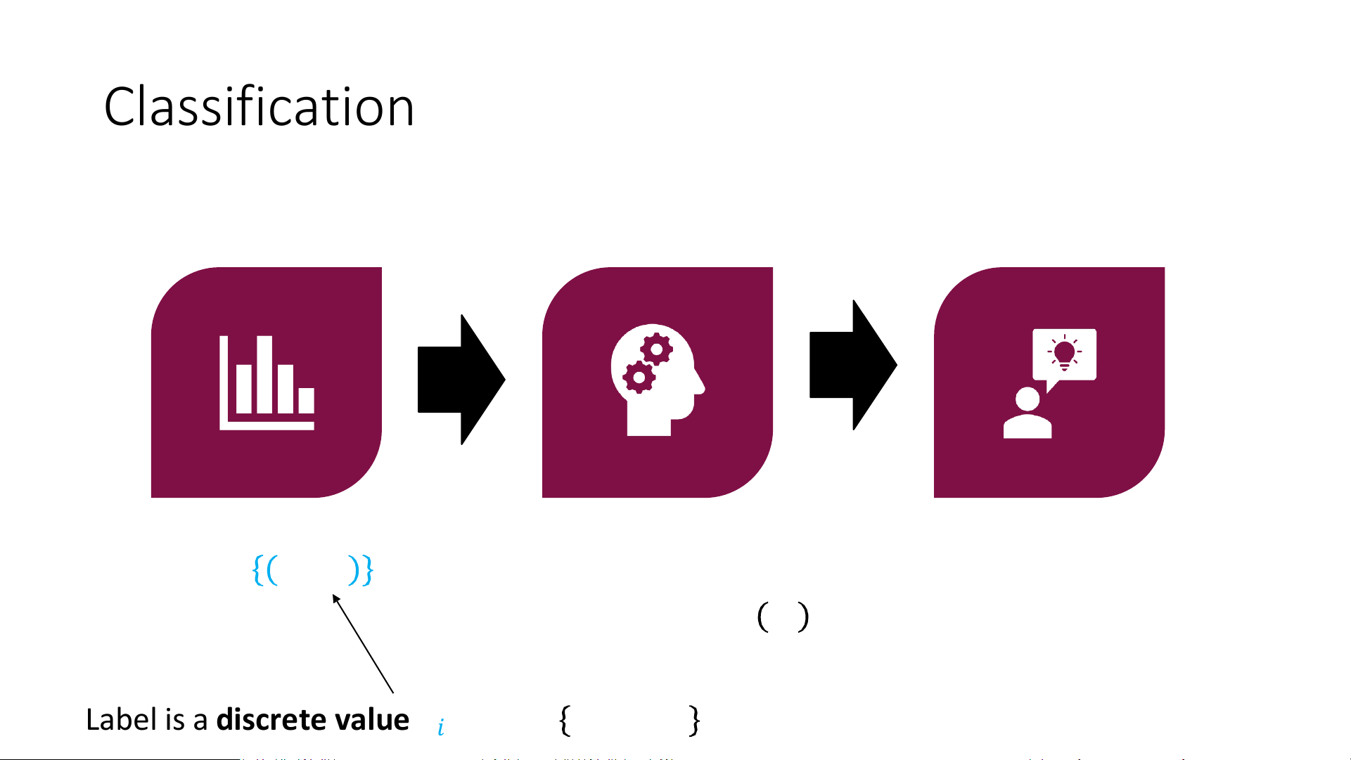
Label is a continuous value 𝑦𝑖 ∈ ℝ Classification Data 𝑍 = 𝑥 𝑛 𝑖, 𝑦𝑖 ෝ 𝜔(𝑍) = arg 𝑚𝑖𝑛 𝑖=1 𝜔𝐿(𝜔;𝑍) Model 𝑓ෝ𝜔(𝑍)
𝐿 encodes 𝑦𝑖 ≈ 𝑓𝜔 𝑥𝑖
Label is a discrete value 𝑦𝑖 ∈ 𝒴 = 𝑐1, … , 𝑐𝑘 (Binary) Classification
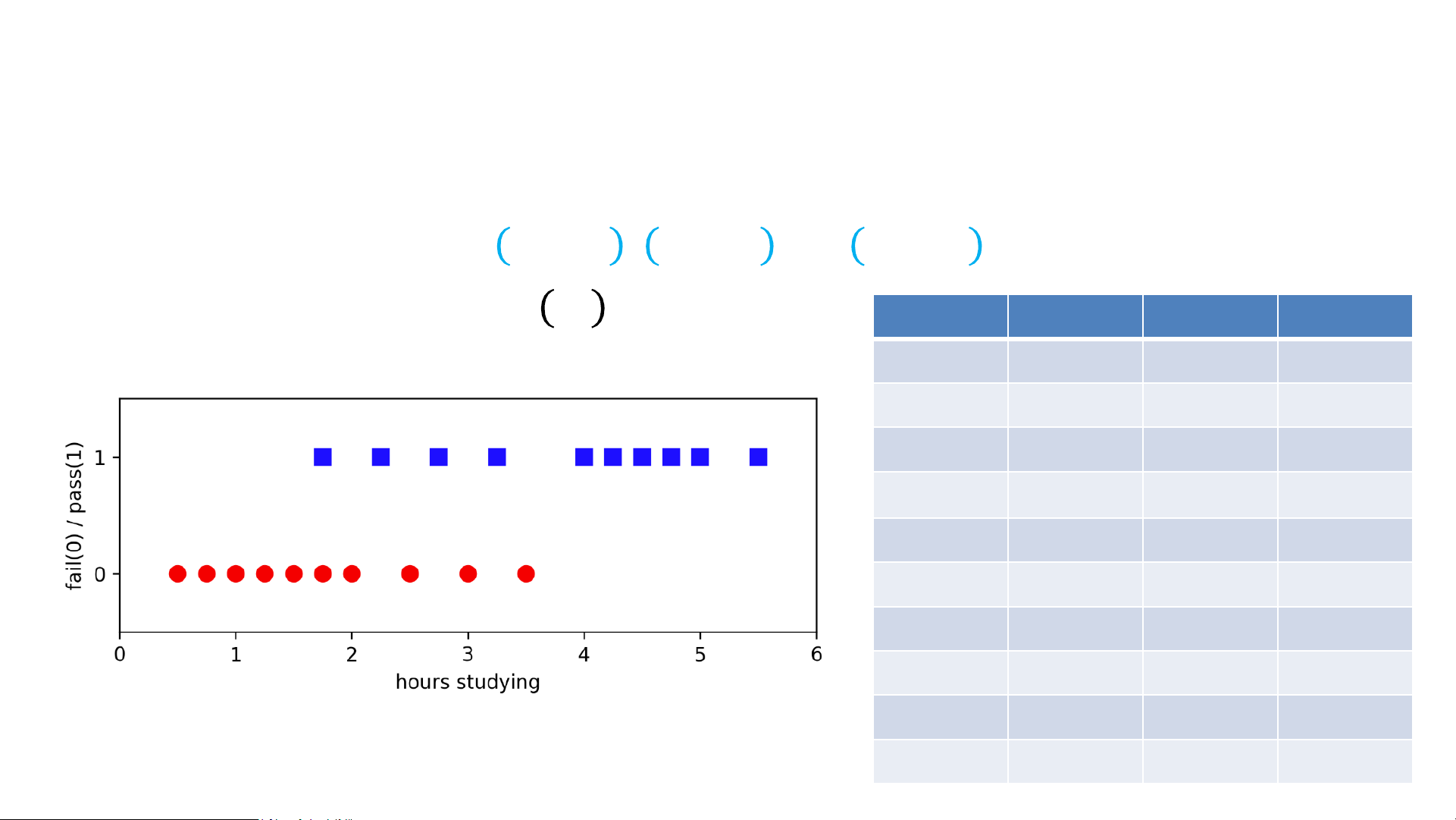
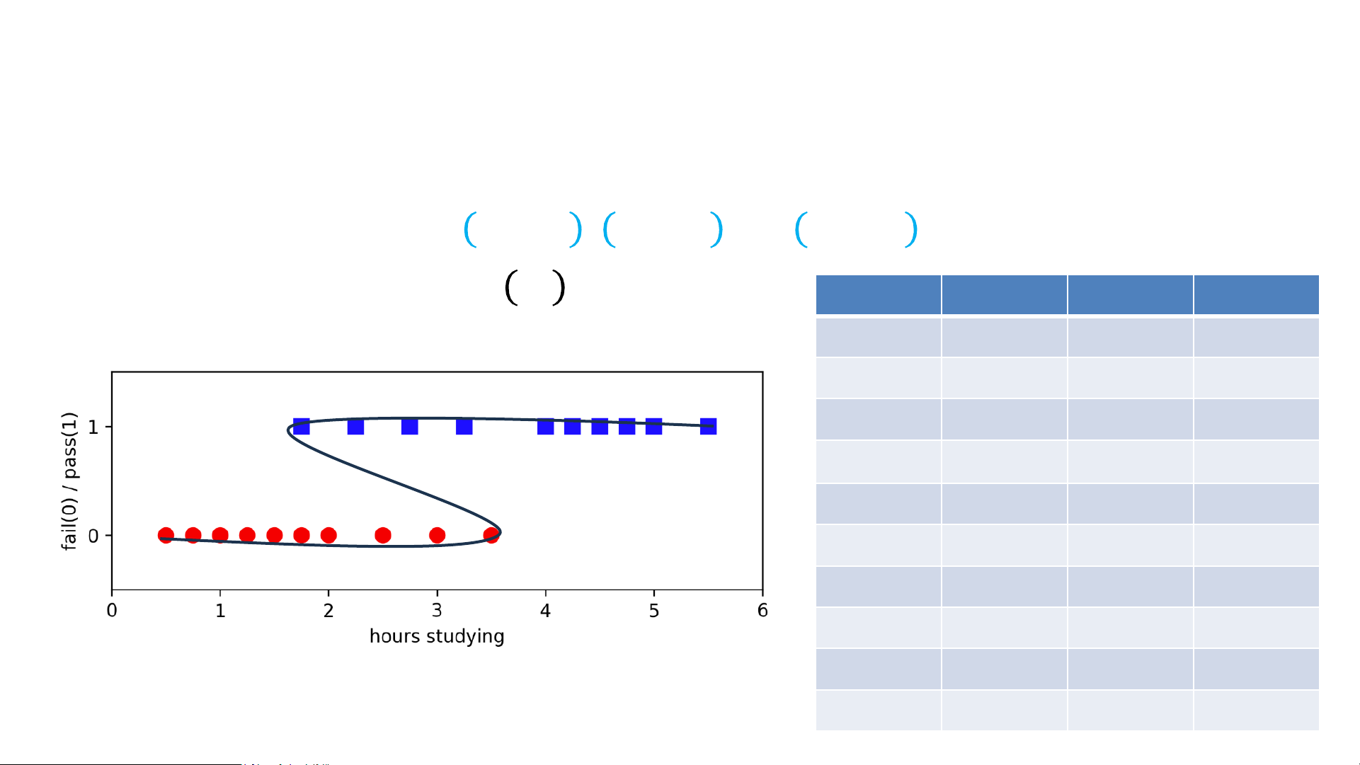
• Input: Dataset 𝑍 = { 𝑥1, 𝑦1 , 𝑥2, 𝑦2 , … , 𝑥𝑛, 𝑦𝑛 }
• Output: Model 𝑦𝑖 ≈ 𝑓𝜔 𝑥𝑖 Hours Pass Hours Pass .5 0 2.75 1 .75 0 3 0 1 0 3.25 1 1.25 0 3.5 0 1.5 0 4 1 1.75 0 4.25 1 1.75 1 4.5 1 2 0 4.75 1 2.25 1 5 1
Example: Fail vs. Pass Exam 2.5 0 5.5 1 (Binary) Classification
• Input: Dataset 𝑍 = { 𝑥1, 𝑦1 , 𝑥2, 𝑦2 , … , 𝑥𝑛, 𝑦𝑛 }
• Output: Model 𝑦𝑖 ≈ 𝑓𝜔 𝑥𝑖 Hours Pass Hours Pass .5 0 2.75 1 .75 0 3 0 1 0 3.25 1 1.25 0 3.5 0 1.5 0 4 1 1.75 0 4.25 1 1.75 1 4.5 1 2 0 4.75 1 2.25 1 5 1
Example: Fail vs. Pass Exam 2.5 0 5.5 1 Loss Minimization View of ML
• Three design decisions
• Model family: What are the candidate models 𝑓? (E.g., linear functions)
• Loss function: How to define “approximating”? (E.g., MSE loss)
• Optimizer: How do we optimize the loss? (E.g., gradient descent)
• How do we adapt to classification?
Hàm sigmoid đc sử dụng trong logistic regression để biến đầu ra thành xác suất và dự đoán xác suất 1 mẫu thuộc về lớp 1.
Sau đó dùng ngưỡng (threshold) để phân loại
P(mắc tiểu đường) = 0.78 → Có nguy cơ
P(mắc tiểu đường) = 0.25 → Không có nguy cơ
Logistic Function for (Binary) Classification
• Input: Dataset 𝑍 = { 𝑥1, 𝑦1 , 𝑥2, 𝑦2 , … , 𝑥𝑛, 𝑦𝑛 }
Loss function: Logistic sử dụng Log Loss / Binary Cross-Entropy • Regression:
Loss=−1/n​∑[ylog(y^​)+(1−y)log(1−y^​)] Trong đó y^ là p (xác suất) • Labels 𝑦
Nếu tính riêng loss của từng mẫu thì bỏ tham số 1/n phía trước đi 𝑖 ∈ ℝ
• Predict 𝑦𝑖 ≈ 𝜔𝖳𝑥𝑖 Trong Logistic Regression, mô hình không trả về 0 hoặc 1 ngay, mà trả về xác suất.
“Hàm mất mát Log Loss phạt rất nặng những trường hợp mô hình dự đoán sai
nhưng lại có mức độ tự tin cao, do đó giúp mô hình học cách đưa ra xác suất hợp • Classification:
lý. Điều này đặc biệt phù hợp với các bài toán dự đoán rủi ro trong y tế. • Labels 𝑦𝑖 ∈ 0, 1
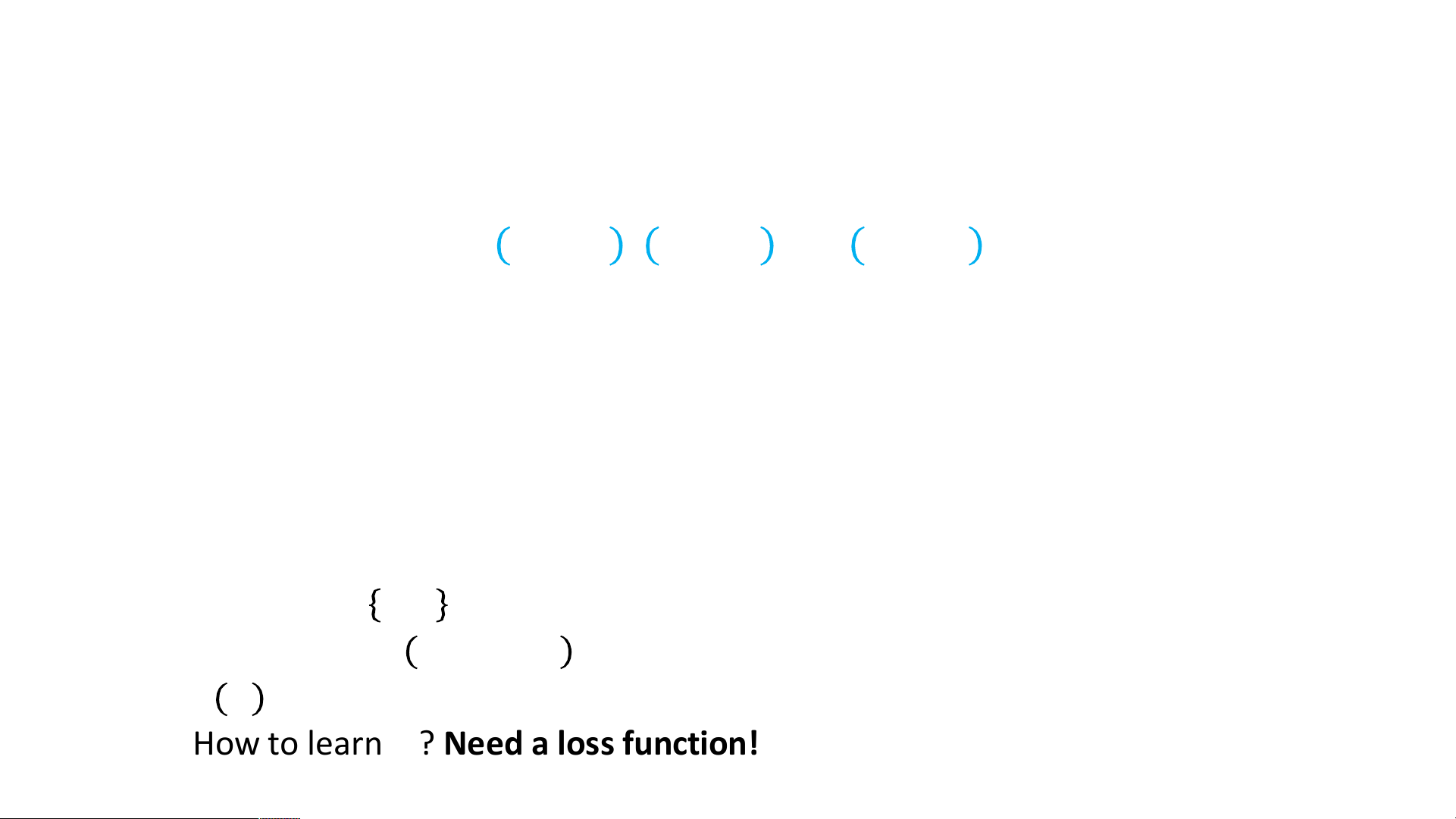
• Predict 𝑦𝑖 ≈ 1 𝜔𝖳𝑥𝑖 ≥ 0
• 1 𝐶 equals 1 if 𝐶 is true and 0 if 𝐶 is false
• How to learn 𝜔? Need a loss function!
z là tổng tuyến tính có trọng số của các đặc trưng đầu vào (linear combination / logit / đầu vào của hàm sigmoid)
Logistic Function for (Binary) Classification
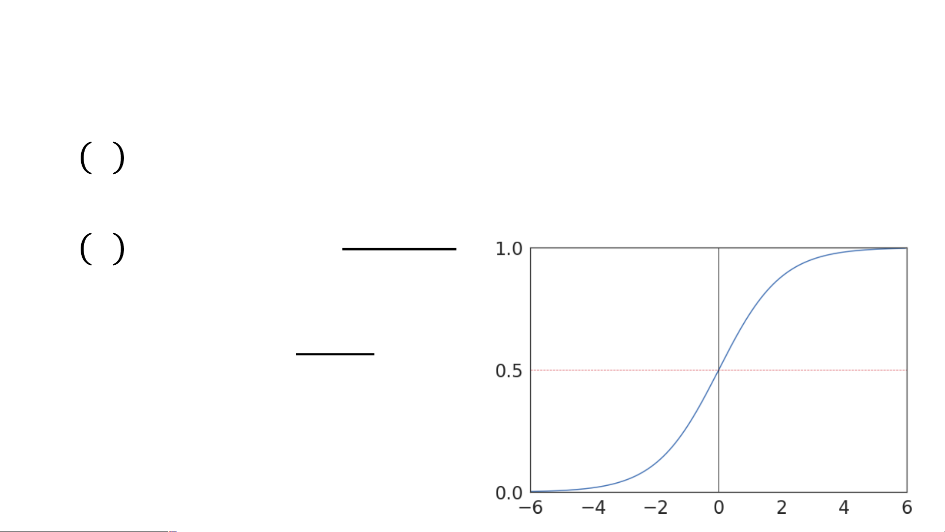
Logistic Regression sử dụng hàm sigmoid để biến đầu ra thành xác suất:
𝑓𝜔 𝑥 = 𝜔𝑇𝑥 ∈ [0, 1]
activation function, sử dụng hệ số e - hệ số tự nhiên Logistic/Sigmoid Function 1
𝑓𝜔 𝑥 = 𝜎(𝜔𝑇𝑥) = 1+𝑒−𝜔𝑇𝑥 σ(z)
z = w0x0 + w1x1 + w2x2 + ...+ wnxn 1 sigma 𝜎(𝑧) =
Giá trị đầu ra nằm trong (0, 1) --> Phù hợp để biểu diễn xác suất 1+𝑒−𝑧 Quy tắc phân loại:
hàm sigmoid biến giá trị bất kì thành xác suất trong (0,1) Sau khi có xác suất:
+ Nếu P≥0.5 → lớp 1 (có bệnh)
+ Nếu P<0.5 → lớp 0 (không bệnh)
Ngưỡng 0.5 có thể thay đổi tùy bài toán (y tế thường ưu tiên Recall)
Logistic sử dụng giả thiết của likelihood: giả thiết tính xác suất để tối ưu hóa w
Huấn luyện mô hình
Likelihood (probability) - Mục tiêu: tìm bộ trọng số 𝑤w sao cho Loss nhỏ nhất
- Phương pháp tối ưu: Xác suất + Gradient Descent
+ Hoặc các biến thể (SGD, LBFGS…) • Model:
𝑝 𝑦 = 1|𝑥; 𝜔 = 𝜎 (𝜔𝑇𝑥) xác suất mắc bệnh biết dữ liệu x và trọng số w
𝑝 𝑦 = 0|𝑥; 𝜔 = 1 − 𝜎 (𝜔𝑇𝑥) xác suất ko mắc bệnh biết dữ liệu x và trọng số w
Bias 𝑏b thường được gộp vào ω
• Likelihood: của toàn bộ dữ liệu 𝑚
𝐿 𝜔 = ෑ 𝜎(𝜔𝑇𝑥 𝑖 ]𝑦(𝑖) ∙ 1 − 𝜎(𝜔𝑇𝑥 𝑖 ]1−𝑦(𝑖) nhãn của mẫu thứ i 𝑖=1 Log-Likelihood & Loss
Log-likelihood đo mức độ phù hợp của mô hình đối với dữ liệu quan sát được. •
Trong Logistic Regression, việc huấn luyện mô hình tương đương với việc tối đa
Log-Likelihood: hóa log-likelihood, hay tương đương với tối thiểu hóa hàm mất mát Log Loss, giúp 𝑚
mô hình đưa ra các dự đoán xác suất hợp lý, đặc biệt vs các bài toán dự đoán rủi ro trong y tế.
𝑙 𝜔 = ෍ 𝑦(𝑖) ln 𝜎(𝜔𝑇𝑥 𝑖
+ (1 − 𝑦 𝑖 )𝑙𝑛(1 − 𝜎(𝜔𝑇𝑥 𝑖 ))] 𝑖=1
Tối đa hóa log-likelihood <--> Tối thiểu hóa Log Loss • Gradient ascent:𝑚
𝜔𝑡+1 = 𝜔𝑡 + 𝛼 ෍(𝑦 𝑖 − 𝜎(𝜔𝑇𝑥 𝑖 ) ∙ 𝑥 𝑖 ) 𝑖=1
Newton’s Method 𝑙′ 𝜔 = 0 𝑙′ 𝜔
𝜔𝑡+1 = 𝜔𝑡 − 𝑙′′ 𝜔 Multi-Class Classification
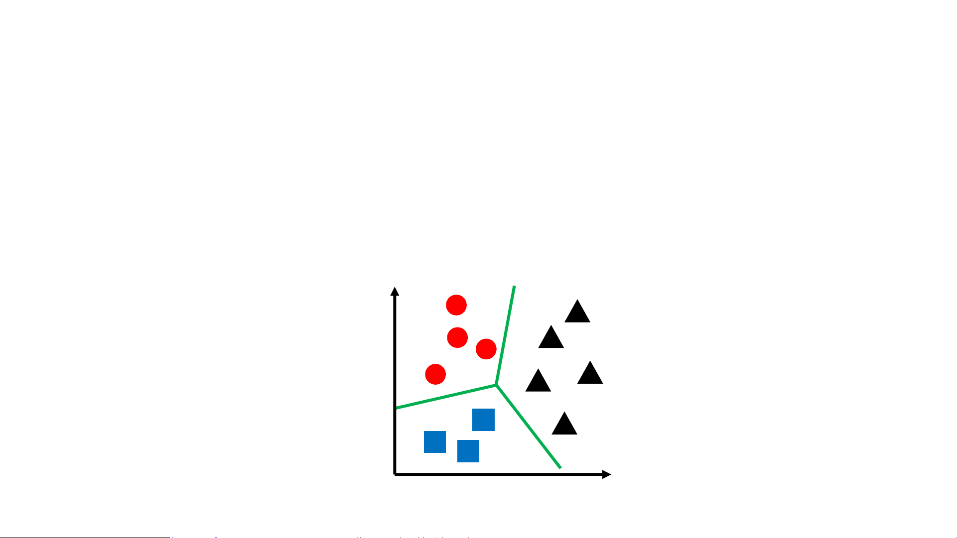
• What about more than two classes?
• Disease diagnosis: healthy, cold, flu, pneumonia
• Object classification: desk, chair, monitor, bookcase
• In general, consider a finite space of labels 𝒴 𝑥2 𝑥1 Multi-Class Classification
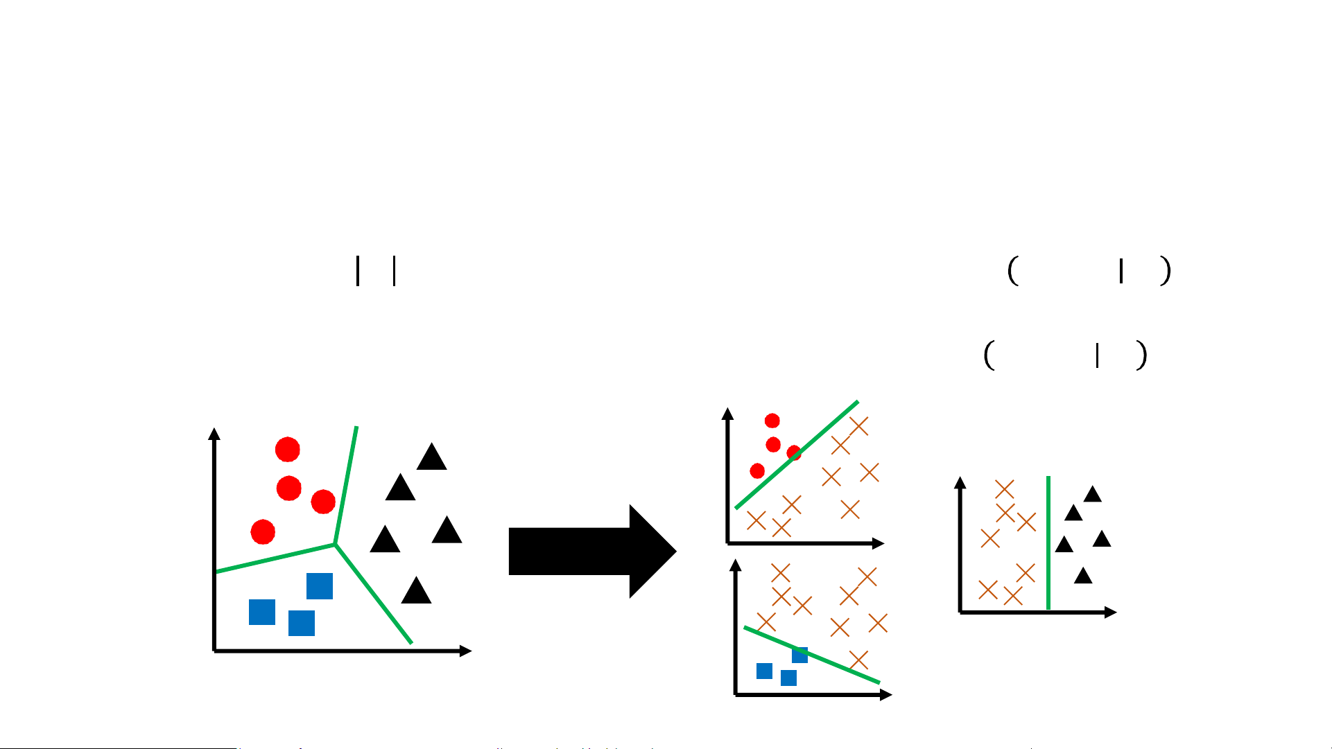
• Naïve Strategy: One-vs-rest classification
• Step 1: Train 𝒴 logistic regression models, where model 𝑝𝜔 𝑌 = 1 𝑥 is 𝑦
interpreted as the probability that the label for 𝑥 is 𝑦
• Step 2: Given a new input 𝑥, predict label 𝑦 = arg max 𝑝𝜔𝑦’ 𝑌 = 1 𝑥 𝑦'
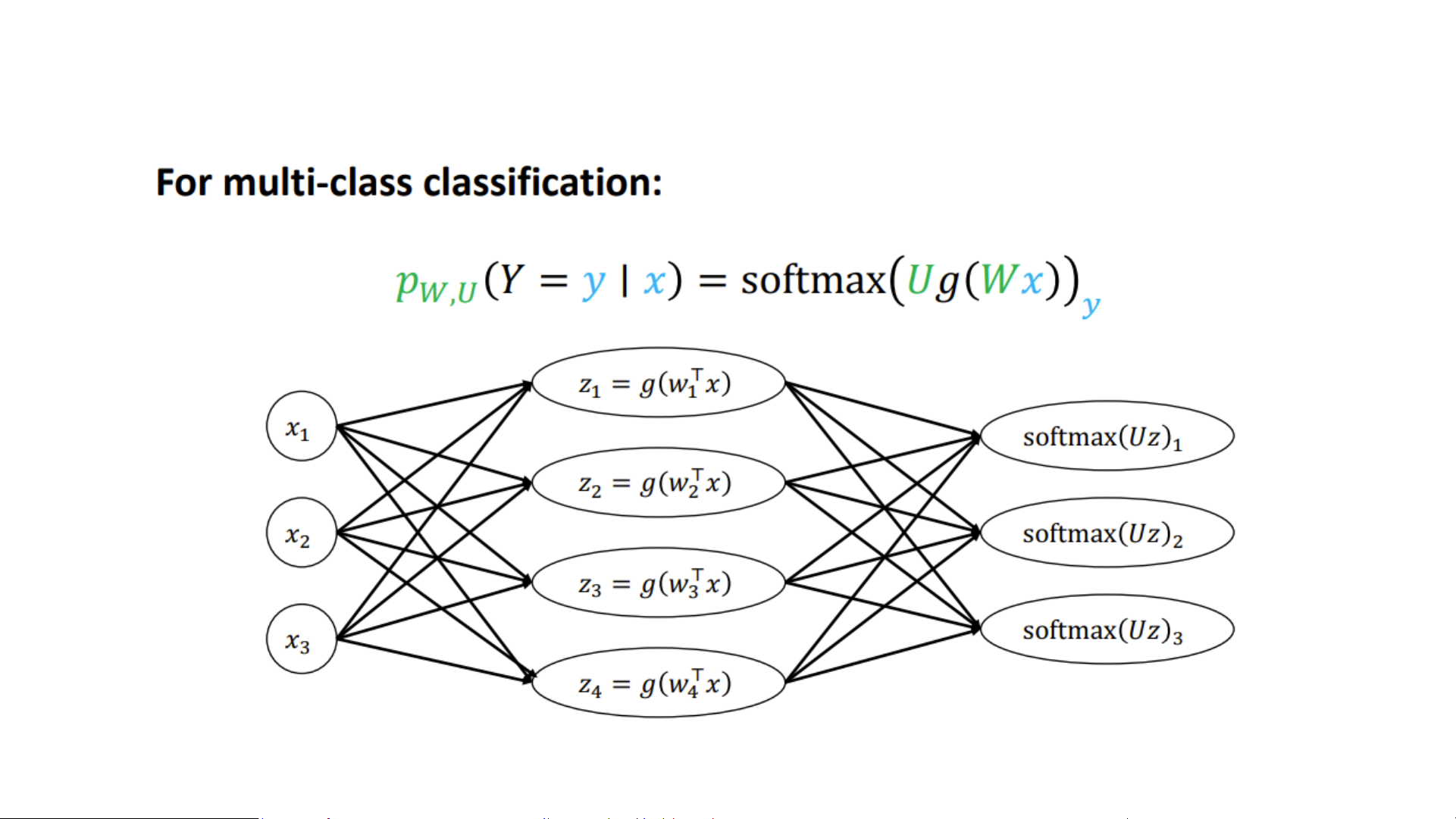
Multi-Class Logistic Regression
• Strategy: For each class 𝑗 = 1, … , 𝑘.
Learn vector 𝜔𝑗 𝛜 𝑅𝑑, give an input feature 𝑥 𝛜 𝑅𝑑 𝑧𝑗 = 𝜔𝑇𝑥
• Convert to probabilities via the softmax function: exp(𝑧 𝑝 𝑗)
𝑗 𝑥 = 𝑃 𝑦 = 𝑗 𝑥 = σ𝑘𝑖=1 exp(𝑧𝑖) 𝑒𝑧1 𝑒𝑧𝑘 • We define softmax 𝑧 … 1, … , 𝑧𝑘 = σ𝑘 σ𝑘 𝑖=1 𝑒 𝑧𝑗 𝑖=1 𝑒 𝑧𝑗
• Then, 𝑝𝛽 𝑦 𝑥 = softmax 𝜔𝖳𝑥, … , 𝜔𝖳𝑥 1 𝑘 𝑦
• Thus, sometimes called softmax regression
Multi-Class Logistic Regression Classification Metrics
• Classify test examples as follows:
• True positive (TP): Actually positive, predictive positive
• False negative (FN): Actually positive, predicted negative
• True negative (TN): Actually negative, predicted negative
• False positive (FP): Actually negative, predicted positive
• Many metrics expressed in terms of these; for example: 𝑇𝑃 + 𝑇𝑁 𝐹𝑃 + 𝐹𝑁 accuracy = error = 1 − accuracy = 𝑛 𝑛 Confusion Matrix Predicted Class Yes No ss Yes a TP FN l C No FP TN Actual Confusion Matrix Predicted Class Yes No ss Yes a 3 TP 4 FN l C No 6 FP 37 TN Actual Accuracy = 0.8 Classification Metrics
• For imbalanced metrics, we roughly want to disentangle:
• Accuracy on “positive examples”
• Accuracy on “negative examples”
• Different definitions are possible (and lead to different meanings)!