Báo cáo thí nghiệm môn Nhiệt động lực học - Truyền nhiệt nội dung tiếng Anh

lOMoARcPSD| 36667950
EXPERIMENT No.1: DETERMINING THE STATE OF MOIST AIR AND
CALCULATING THE HEAT BALANCE OF AIR DUCT
1.1 EXPERIMENTAL OBJECTIVES AND REQUIREMENTS
1.1.1 Experimental objectives
- Knowing how to measure the temperatures (dry and wet bulb temperature), air flow, pressure and volume.
- Understanding the cooling and dehumidifying process of humid air.
- Understanding the working and principle and main components of a basic refrigeration cycle.
- Calculating the heat balance in air duct. 1.1.2 Requirements
Students carefully read the following sections in theory before doing the experiment: - Pure substance. - Moist air. - Refrigeration cycle.
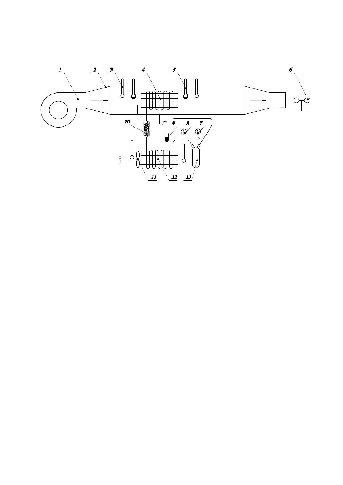
1.2 EXPERIMENTAL DESCRIPTION
1.2.1 Equipment and supplies - Air duct. - Refrigeration cycle.
- Dry and wet bulb thermometers. - Anemometer. - Volume measuring device. - Vernier caliper. 1.2.2 Description
Moist air is blown through a cooling of a refrigeration system. The dry and wet bulb
thermometers are put in front of behind the cooling coil to determine the state of humid air. lOMoARcPSD| 36667950
At the outlet of air duct, an anemometer is used to measure the speed and temperature of moist air.
Refrigerant in refrigeration system is R22:
1.3 REQUIREMENTS OF EXPERIMENT 1. Blower 5. Wet 9. Measuring flask 13. Compressor thermometer 2. Wind channel 6. Speedometer, 10. Valve wind temperature 3. Dry 7. Volatile 11. Fan thermometer manometer Condenser 4. Evaporator 8. Condensation 12. Condenser manometer
- Using dry and wet bulb thermometers to determine the state of moist air at the inlet
(it is also the surrounding temperature) and outlet of the cooling coil.
- Using anemometer to measure the velocity and temperature at outlet of air duct in order to estimate airflow.
- Determining the evaporating and condensing temperature of refrigeration system.
From above data, student determines:
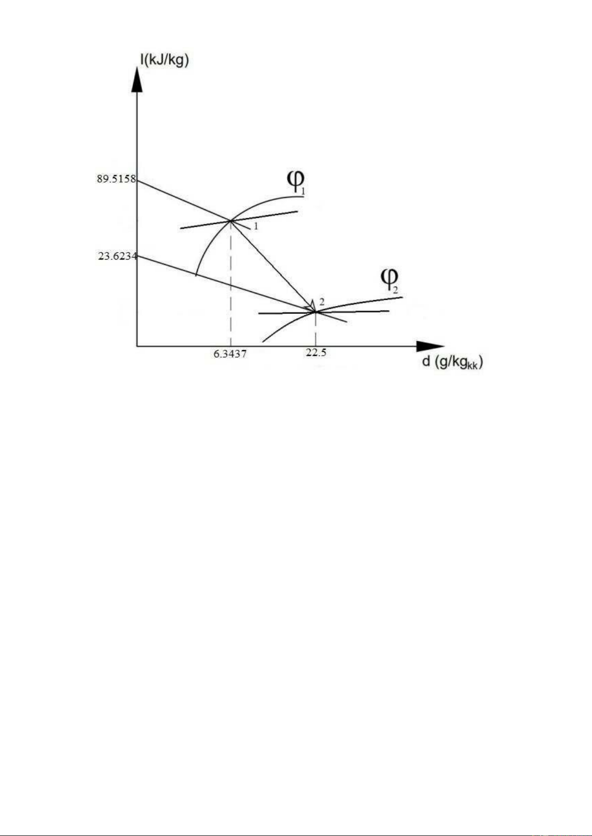
- Demonstrating the processes of humid air on the t-d diagram (or I-d).
- The heat released when humid air passes through the cooling coil.
- Moisture is removed at cooling coil according to theoretical calculations and experiments. lOMoARcPSD| 36667950
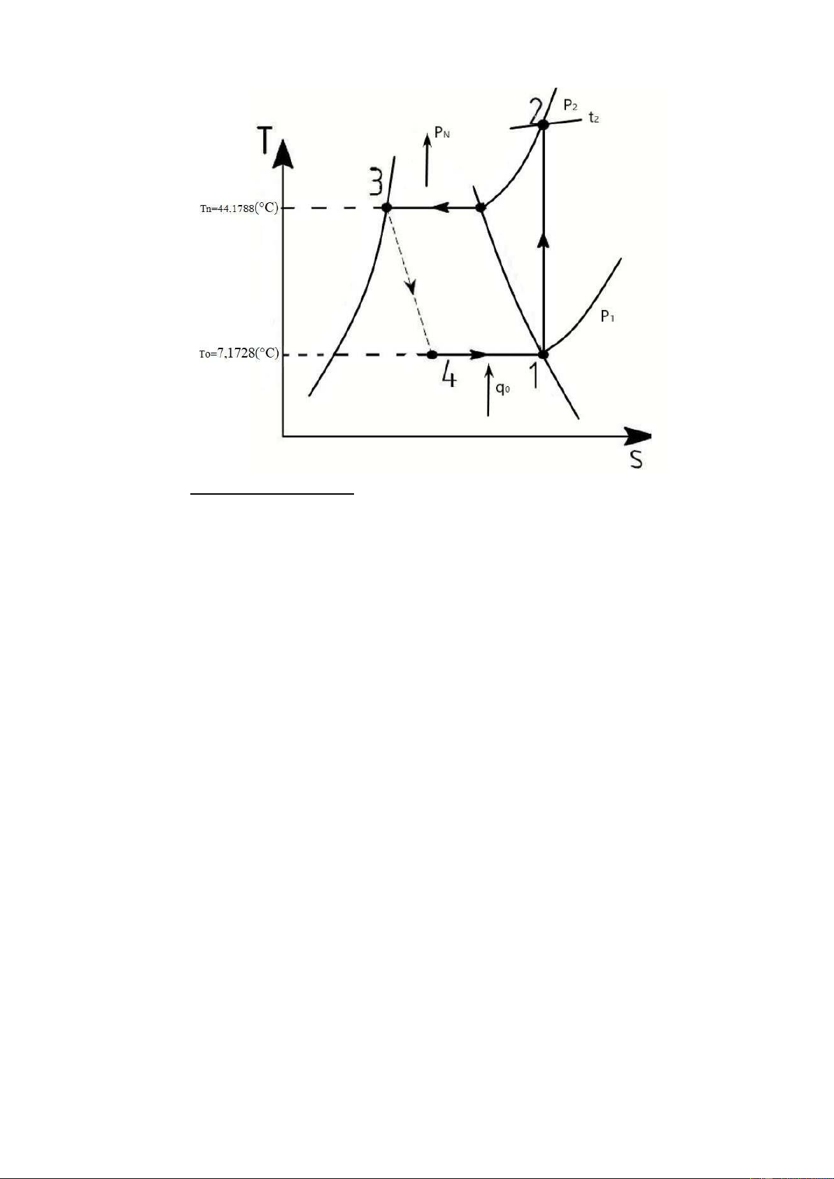
- Demonstrating the states of refrigerant on the T-s diagram (corresponding with
theoretical refrigeration cycle, neglecting the superheat and subcooling processes). 1.4 EXPERIMENTAL DATA
When the system operates at steady state, the condensing water appears on the cooling
coil, student starts doing the experiments with the following requirements:
Student conducts two experiments (Note: after getting the experimental data, student
changes the airflow through the cooling coil).
Experiment 1: Experimental time is 15 minutes; the number of data collection are 3
times. Experiment 2: Experimental time is 10 minutes; the number of data collection are 4 times.
SAMPLE CALCULATION: Using data from Experiment 1 of the 1st time Experiment 1
Moist air at the inlet of coil
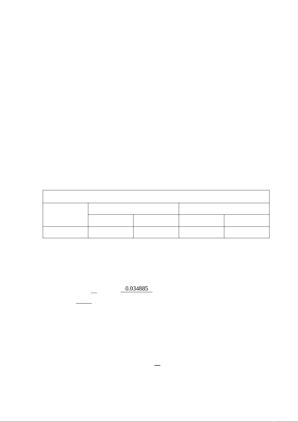
Moist air at the outlet of coil tk(°C) tư(°C) tk(°C) tư(°C) The 1sttime 31 26.5 16 15 - Determine d
Air after evaporator; tư=26.5(°C)=> Use table => Ph=0.034885¯¿ Phkg d=0.622×
=0.622× =0.0225 P−Ph 1−0.034885 kgkk
d=22.5g/kgkk (Air pressure p = 1 bar)
Similarly, we can determine d for the gas behind the evaporator kg d=0.0108 =10.8g/kgkk kgkk lOMoARcPSD| 36667950 - Determine I: Air after Condenser:
I=tk+d(2500+2.tk)=31+0.0225×(2500+2.31)=88.645kJ/kg
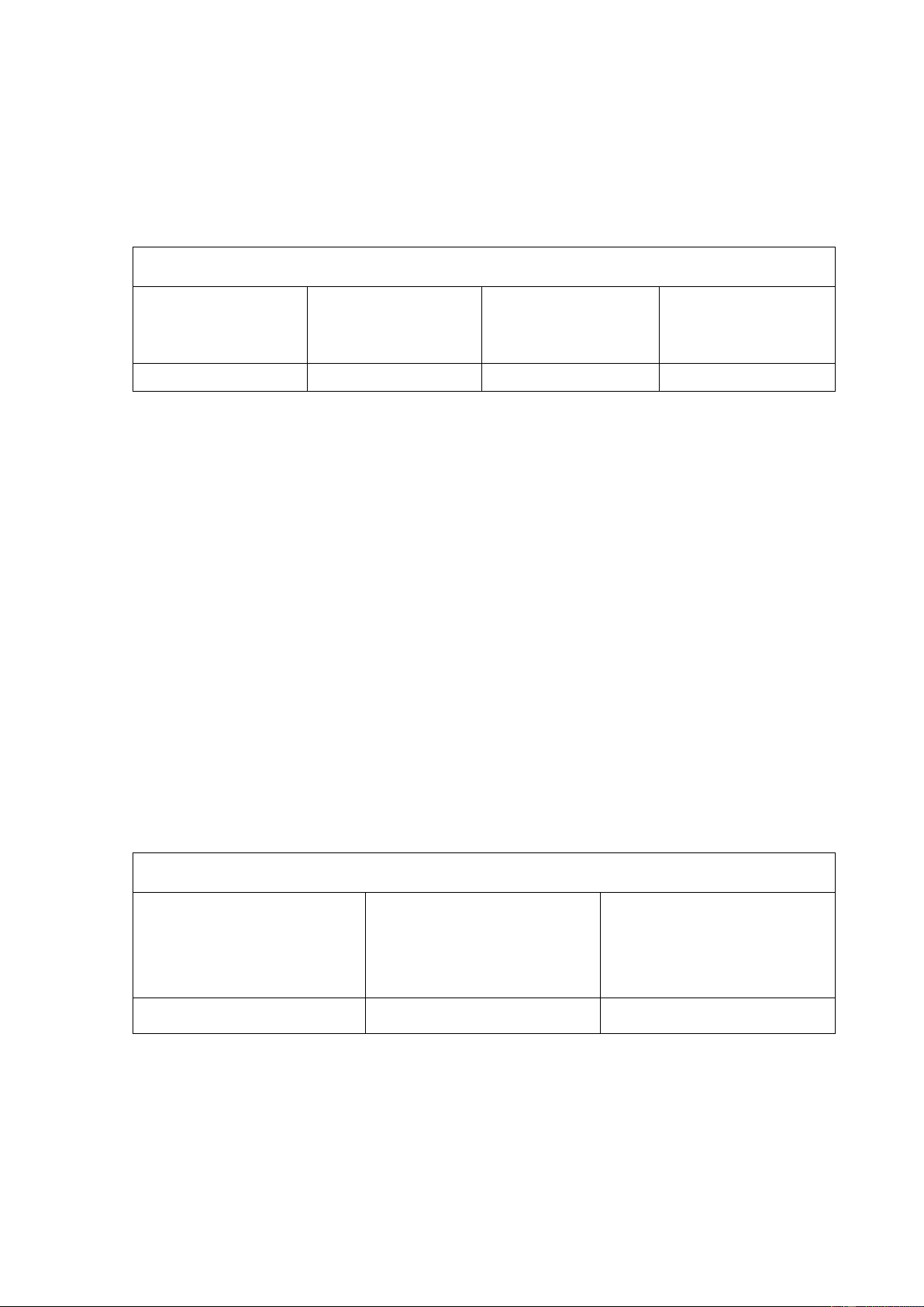
Similarly, we can determine I for the gas behind the condenser I=433456kJ/kg Experiment 1 Velocity at outlet Temperature at Water condensed of air duct v(m/s) outlet of air (ml) duct(°C) The 1sttime 4.20 17 196
- Determine the amount of moisture separated according to the calculation Vtt Gkk=V × F×ρ
V: average velocity at outlet of air duct F is acreage of out duct (m2)
F=0.105×0.105=0.01103m2 ρ: density of air
Gkk=4.20×0.01103×1.2176=0.0564 kg/s
- Determine the amount of air released when passing through the indoor unit Q
Q=Gkk×(Itb1−Itb2)=0.0564×(88.645−43.3456)=2.5549kW Experiment 1 Evaporating pressure Condensing (Gauge) pressure (Gauge) (kgf/cm2) (kgf/cm2) The 1sttime 5.5 16.5
- Evaporating temperature (°C) => Use table: ts=7.1728(°C)
- Condensing temperature (°C) => Use table: tn=45.2764(°C)
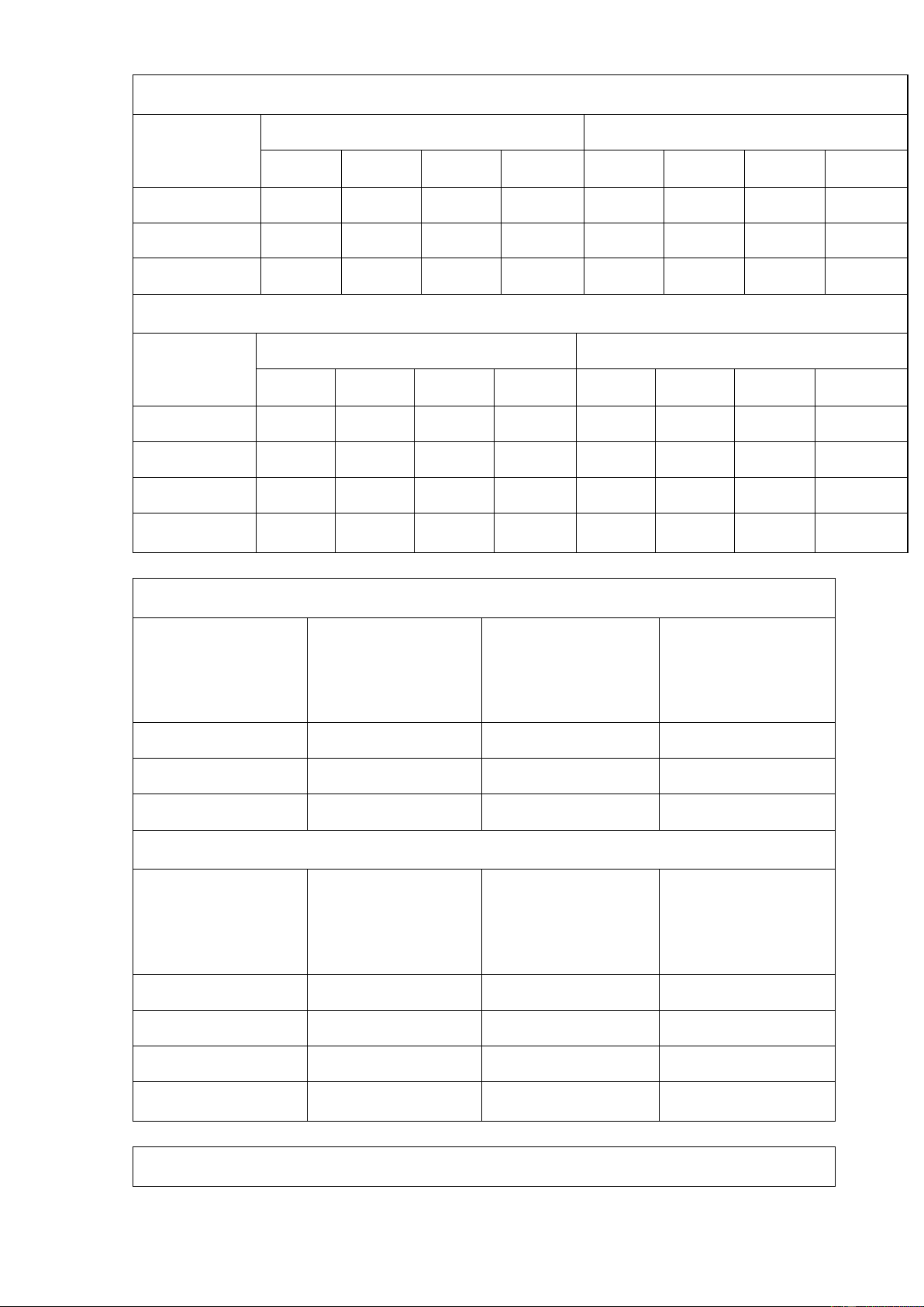
Table 2 & 3: The state parameters of moist air lOMoARcPSD| 36667950 Experiment 1
Moist air at the inlet of coil
Moist air at the outlet of coil tk(°C) tư(°C) d(g/kg) I(kJ/kg) tk(°C) tư(°C) d(g/kg) I(kJ/kg) The 1sttime 31 26.5 22.5 88.645 16 15 10.8 43.3456 The 2ndtime 31 26 21.8 86.8516 14 13 9.56 38.1677 The 3rdtime 31 27 23.2 90.4384 13 13 9.56 37.1487 Experiment 2
Moist air at the inlet of coil
Moist air at the outlet of coil tk(°C) tư(°C) d(g/kg) I(kJ/kg) tk(°C) tư(°C) d(g/kg) I(kJ/kg) The 1sttime 31.5 26.5 22.5 89.1675 7 6 5.901 21.83511 The 2ndtime 32 26.5 22.5 89.69 8 7 6.34 23.95144 The 3rdtime 32 26.5 22.5 89.69 8 8 6.79 25.0836 The 4thtime
Table 4 & 5: Other parameters of moist air Experiment 1 Velocity at outlet Temperature at Water condensed of air duct v(m/s) outlet of air (ml) duct(°C) The 1sttime 4.20 17 196 The 2ndtime 4.31 16.5 254 The 3rdtime 4.27 16 266 Experiment 2 Velocity at outlet Temperature at Water condensed of air duct v(m/s) outlet of air (ml) duct(°C) The 1sttime 2.806 10 100 The 2ndtime 2.576 9 198 The 3rdtime 3.076 11 230 The 4thtime
Table 6 & 7: The parameters of refrigeration cycle Experiment 1 lOMoARcPSD| 36667950 Evaporating Evaporating Condensing Condensing pressure temperature pressure temperature (Gauge) (°C) (Gauge) (°C) (kgf/cm2) (kgf/cm2) The 1sttime 5.5 7.1728 16.5 45.2764 The 2ndtime 5.5 7.1728 17 46.6484 The 3rdtime 5.5 7.1728 17 46.6484 Experiment 2 Evaporating Evaporating Condensing Condensing pressure temperature temperature (Gauge) (°C) pressure (°C) (kgf/cm2) (Gauge) (kgf/cm2) The 1sttime 5.5 7.1728 16 43.9044 The 2ndtime 5.5 7.1728 16.1 44.1788 The 3rdtime 5.5 7.1728 16.2 44.4532 The 4sttime
1.5 COMMENTS OF EXPERIENCE RESULTS
1.5.1 Represent the process of changing the state of the air on the t-d (or I-d) graph.
+ Experiment 1: Use the average value of the first experiment to draw a graph.
+ Experiment 2: Use the average value of the second experiment to draw a graph. lOMoARcPSD| 36667950
1.5.2 The amount of moisture separated from the indoor unit according to the calculation and actual value commented.
The amount of water separated from the air deviates much from the theory (40-60%). Reason:
- The machine has been used for a long time, error in taking out water, error in measuring tools.
- Unstable space affects the experimental process (crowded people gather) should influence the results.
1.5.3 Representing the states of the refrigerant on the T-s graph (corresponding to the
physical refrigeration cycle theory, ignoring superheat too cold.)
Since there was not much change in the cold cycle between the two experiments (using
the same experimental system), so we plot the same graph for both experiments to get the average data to draw. lOMoARcPSD| 36667950
EXPERIMENT No.2: DETERMING THE COEFFICIENT OF
PERFORMANCE (COP) OF A REFRIGERATION CYCLE USING
AIRCOOLED CONDENSER AND AIR-COOLED EVAPORATOR
2.1EXPERIMETNAL OBJECTIVES AND REQUIREMENTS
2.1.1 Experimental objectives
- To help students combine theoretical and practical knowledge.
- To know the fundamental principle of the air conditioning system incorporating some auxiliary devices.
- To help students measure the parameters such as temperature, pressure and
calculate the actual heat and COP. 2.1.2 Requirements
- Students must understand the refrigeration cycle.
- Knowing to apply the mathematic formulas for refrigeration cycle.
2.2 EXPERIMENTAL DESCRIPTION
2.2.1 Equipment and supplies
- The model of air conditioning system - The temperature sensors lOMoARcPSD| 36667950 2.2.2 Description
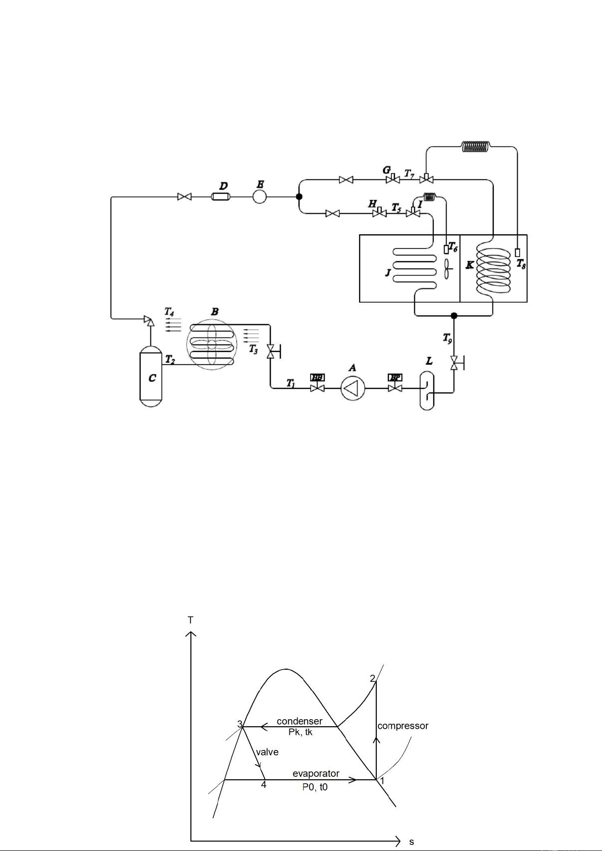
To cool the air in the air-conditioning room, the diagram of the experimental model
using refrigeration system with refrigerant of R12 is illustrated in figure 1. The
compressor (A) compresses the vapor of R12 from the evaporating pressure P0 to the
condensing pressure Pk. Then, this vapor is condensed to liquid at the air-cooled
condenser (B) before entering the high-pressure receiver (C). The liquid of R12 at the
receiver (C) passes through the expansion valve (I) where the pressure is reduced from
Pk to P0 and then this vapor goes to the air-cooled evaporator (J). The heated refrigerant
vapor at (J) is sucked into the compressor (A) and the principle of operation is repeated again. Therefrigeration cycle is representedin the logp-I and T- lOMoARcPSD| 36667950
Therefrigeration cycle representedin T-s graph
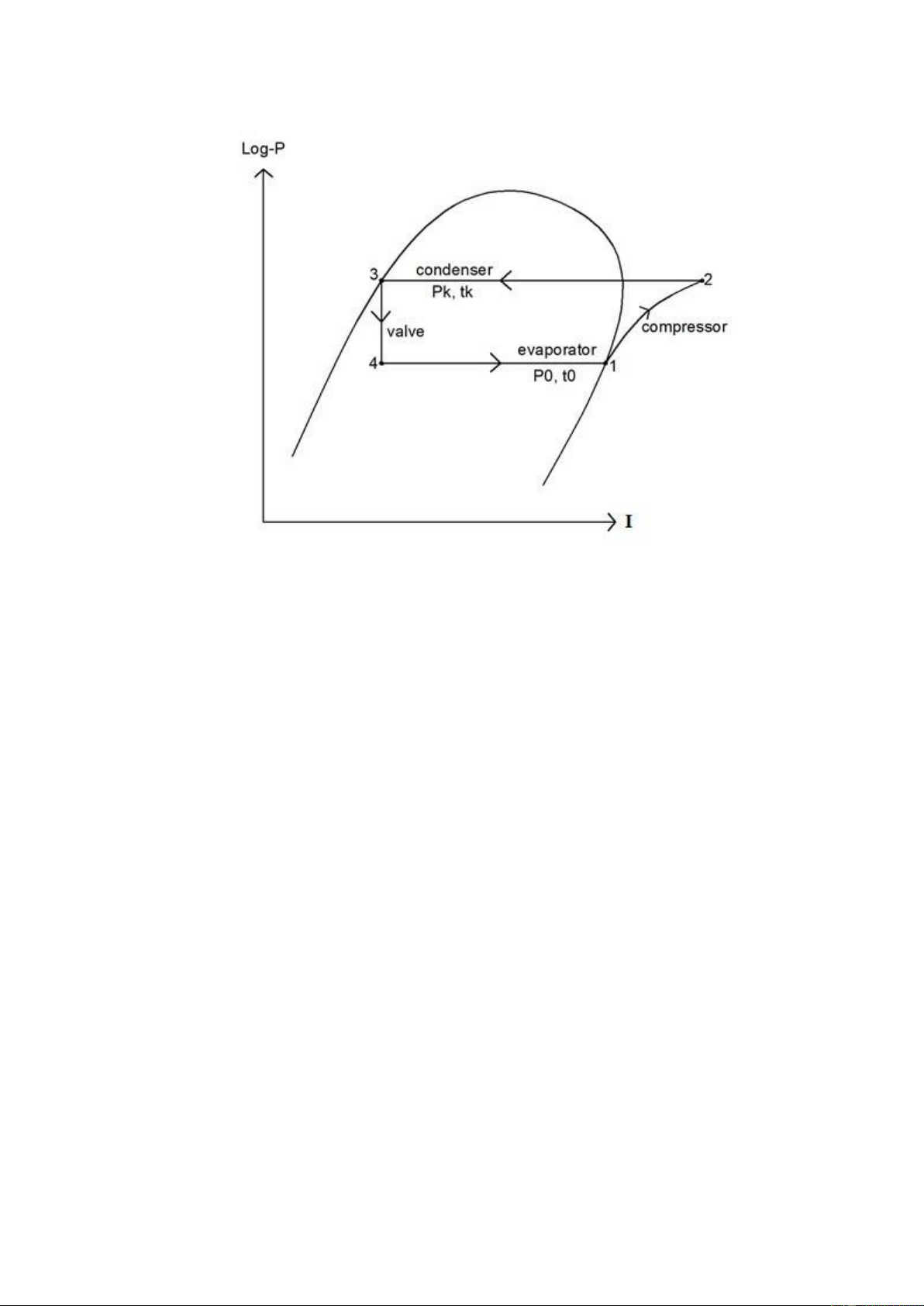
The refrigeration cycle represented in LogP-I graph
1-2: The process of diabatic compression in the compressor.
2-3: The process of isobaric condensation in the condenser.
3-4: The process of constant - enthalpy expansion in the throttling valve.
4-1: The process of isobaric evaporation in the evaporator.
The measurement positions of temperature and pressure in the refrigeration cycle
The manometers P1 and P2 are used to measure the suction and discharge pressures at
the throttling valve, respectively and also the discharge pressure of the compressor.
The temperatures of the R12 refrigerant entering and leaving the air-cooled condenser
(B) are measured by the sensors of T1 and T2.
The temperatures of the air entering and leaving the air-cooled condenser (B) are
measured by the sensors of T3 and T4, respectively.
The temperatures of the R12 refrigerant entering and leaving the air-cooled evaporator
(B) are measured by the sensors of T5 and T9, respectively.
The temperature of the air in the air-conditioning room is measured by the sensors of T6. lOMoARcPSD| 36667950 2.3 EXPERIMENTAL TASKS
In this experiment, the students are required to collect the data on the suction and
discharge pressures; the temperatures of the refrigerant entering and leaving the
aircooled condenser, the temperatures of the refrigerant entering and leaving the
aircooled evaporator, the temperatures of the air entering and leaving the air-cooled
condenser and the temperatures of the air entering and leaving the air-cooled evaporator.
Then, combining with the computing results to determine:
- The state properties of the actual refrigeration cycle.
- COP (ε) of the theoretical and actual refrigeration cycle.
- The heat load of the air-cooled condenser, Qk.
- The necessary air flow to receive the heat rejection from the condenser, Gkk. 2.4 EXPERIMENTAL DATA
Table 1: The measured data of the refrigerant in the refrigeration cycle
Absolute pressure (bar)
At the discharge line of the compressor
At the suction line of the compressor (p0) (pk) 10 2.5 9.8 2.2 9.7 2.0
Table 2: The measured temperatures of air
Air Temperature (°C) Surrounding At the outlet of At the air
temperature (T a) condenser (T4)
conditioning room (T6) 30 33 17 30 34 10 30 34 10
2.5 CALCULATING SECTION lOMoARcPSD| 36667950
a. Determining the state properties of the refrigerant
From Table 1 and the thermodynamic properties of saturated refrigerant R12 and the
thermodynamic properties of superheated refrigerant R12, we can fill in Table 3 below:
Table 3: The properties of R12 in refrigeration cycle State Parameter 1 2 3 4 Pressure p¿ 2.0 9.7 9.7 2.0
Temperature t (°C ) -12.53 49.17 40.19 -12.53
Enthalpy i(kJ /kg) 282.6940 310.9377 174.1693 174.1693
Entropy s(kJ /kg. K) 2.3512 2.3512 1.9150 1.9150
b. Calculating the heat load of the air-conditioning room
The heat load of the air-conditioning room is the amount of heat from the surrounding
environment that passes through the walls due to the difference in the temperature.
i. Calculating the heat flux q(W /m2) that transfers across each wall as follows: qf T3−T6 1 δi 1 ∑ With:
δi: Thickness of layer i, m λi: Thermal conductivity of the layer i, W/mK α1: The
convection heat transfer coefficient outside the air-conditioning room, W/m2K
Select α1=6W /m2 K
α2: The convection heat transfer coefficient inside the air-conditioning room, W/m2K
Select α2=12W/m2K Material
Thickness (δ), (mm)
Thermal conductivity (λ), W/mK Mica 3.74 0.58 Insulation material 10 0.04 Wood 4.32 0.15 Steel 1.88 45 lOMoARcPSD| 36667950 Front wall: Mica
q1= 1 T3δ−mT6 1 + + α1 λm α2 ¿ =77.99(W /m2) + + 6 0.58 12
Back wall: Wood and insulation material q2= 1 δT3−Tδ6 1 + + +
α1 λw λℑ α2 ¿ =37.82(W /m2) + + + 6 0.15 0.04 12 Top wall: Wood q3=
1 T3δ−wT6 1 = 1 4.3230×−1010−3 1 =71.74(W /m2) + + + + α1 λw α2 6 0.15 12
Bottom wall: Wood and insulation material
T3−T6 q4= + + + α1 w ℑ α2 ¿ =37.82(W /m2) + + + 6 0.15 0.04 12 lOMoARcPSD| 36667950
Left wall: Wood and insulation material
q5= 1 Tδ 3−Tδ6 1 + + +
α1 λw λℑ α2 ¿ =37.82(W /m2) + + + 6 0.15 0.04 12 Right wall: Steel
q6= 1T3−δsT61 + + α1 λs α2 ¿ =79.99(W /m2) + + 6 45 12
ii. The amount of heat transfer across each wall (W) Q=F ×q
F is the area of flat wall, m2 Wall Dimension (m x m) Front 0.8 x 0.4 Back 0.8 x 0.4 Top 0.8 x 0.4 Bottom 0.8 x 0.4 Left 0.4 x 0.4 Right 0.4 x 0.4
Front wall: Q1=F1×q1=0.8×0.4×77.99=24.96(W)
Back wall: Q2=F2×q2=0.8×0.4×37.82=12.10(W)
Top wall: Q3=F3×q3=0.8×0.4×71.74=22.96(W) lOMoARcPSD| 36667950
Bottom wall: Q4=F4×q4=0.8×0.4×37.82=12.10(W)
Left wall: Q5=F5×q5=0.4×0.4×37.82=6.05(W)
Right wall: Q6=F6×q6=0.4×0.4×79.99=12.80(W) iii. The heat
load of the air-conditioning room (W)
Q0=∑ Q=24.96+12.10+22.96+12.10+6.05+12.80=90.97(W)
c. Determining the flow rate of R12 (kg/s) in refrigeration cycle (Ignoring the heat
loss to the surrounding environment) Q0 GR12= i1−i4 −3 90.97×10 −4 ¿ =8.38×10 (kg /s) 282.6940−174.1693
d. Determining the heat load of the condenser Qk(kW)
Qk=GR12× (i2−i3)=8.38×10−4×(310.9377−174.1693)=0.11461(kW)
e. Determining the air flow rate passing through the condenser (kg/s)
Qk=Gair×C pair ×Δt=Gair×C pair ×(tout−t¿)=Gair ×Cpair ×(T4−T a) Qk 0.11 →Gair= = =0.03(kg /s) C p ×(T air 4−T3) 1×(34−30)
f. Determining the adiabatic compression work of compressor W (kW)
W=GR12× (i2−i1)=8.38×10−4×(310.9377−282.6940)=0.02366(kW) lOMoARcPSD| 36667950
g. Determining (COP)ϵ Q0 90.97×10−3 COP=ϵ= = =3.84 W 0.02366 lOMoARcPSD| 36667950
EXPERIMENT No. 3 : CALCULATION OF HEAT EXCHANGES
3.1EXPERIMENTAL OBJECTIVES AND REQUIREMENTS
3.1.1 Experimental objectives
- Observing the heat transfer processes of helical-coil heat exchanger and shell and tube heat exchanger.
- Calculating the heat exchanger efficiency and understanding the factors that
affect the heat transfer processes. 3.1.2 Requirements
Students carefully read the following contents before conducting the experiments:
- The types of heat transfer: conduction, convection, radiation.
- The formula for calculating the heat rate that water received and rejected.
- The formula for calculating the overall heat transfer coefficient and Reynold number.
3.2 EXPERIMENTAL DESCRIPTION
3.2.1 Equipment and supplies
The equipment consists of two heat exchangers (helical-coil and shell and tube heat
exchanger) in which two fluids flow in parallel flow or in counter flow.
Figure 1: Helical-coil heat exchanger lOMoARcPSD| 36667950
Figure 2: Shell and tube heat exchanger
Figure 3: Flowmeters of hot water (FI1) and cold water (FI2)
- There are 4 temperature sensors which are used to measure the temperature of hot
and cold water at inlet and outlet of the heat exchanger. The temperatures are shown on the display screens. Technical specifications:
a. The helical - coil heat exchanger: -
The helical-coil heat exchanger has the heat transfer area of 0.1m2, symbol E2. -
The coil made of stainless steel AISI 316. Other parameters include the outside
diameter of 12mm, the thickness of 1mm, the length of 3500mm. lOMoARcPSD| 36667950 -
The outside tube made of borosilicate glass with the inside diameter of 100mm.
b. The shell and tube heat exchanger: -
The shell and tube heat exchanger has the heat transfer area of 0.1m2, symbol E1. -
There are five tubes which made of stainless steel AISI 316. Other parameters
include the outside diameter of 10mm, the thickness of 1mm, the length of 900mm. -
The shell made of borosilicate glass with the inner diameter of 50mm. -
There are 12 baffles and baffle cut of 25% shell diameter. 3.2.2 Description
Before starting the experiment: -
Checking the inlet and outlet of water to make sure that they are connected to water pipe. - Checking the power source. - Checking the hot water tank. - Closing the exhaust valves. -
Turning on the digital temperature switch. -
Turning on the hot and cold water pump. -
The hot and cold water flow through the heat exchanger. The temperatures are shown on display screens. 3.3 EXPERIMENTAL TASKS
Conducting the following experiments and collecting data:
a. Running E1 (Shell and tube heat exchanger) in parallel flow:
Opening valves as V1, V6, V7, V8 and V10.
Closing valves as V2, V3, V4, V5, V9 and V11.
b. Running E1 (Shell and tube heat exchanger) in counter flow:
Opening valves as V1, V6, V7, V9 and V11. lOMoARcPSD| 36667950
Closing valves as V2, V3, V4, V5, V8 and V10.
c. Using E2 (Helical-coil heat exchanger) in parallel flow:
Opening valves as V3, V4, V5, V8 and V10.
Closing valves as V1, V2, V6, V7, V9 and V11.
d. Using E2 (Helical-coil heat exchanger) in counter flow:
Opening valves as V3, V4, V5, V9 and V11.
Closing valves as V1, V2, V6, V7, V8 and V10.
- Changing the hot and cold water flow rate by adjusting the valves as mentioned
above. After adjustment, waiting for 2-3 minutes until the temperature sensors are
stable, students start getting the experimental data. 3.4 EXPERIMENTAL DATA
E1 (shell and tube heat exchanger) in PARALLEL flow: Test FI1 FI2 TI1 TI2 TI3 TI4 ∆T ∆T (hot) (cold) 1 800 800 47.7 44.7 32.9 36.1 3 3.2 2 700 800 50.7 46.9 33.5 37.2 3.8 3.7 3 900 800 51.8 48.4 34.1 38.2 3.4 4.1 4 800 700 51.4 48.1 34.6 38.7 3.3 4.1 5 800 900 51.1 47.8 35.1 38.4 3.3 3.3
E1 (shell and tube heat exchanger) in COUNTER flow: Test FI1 FI2 TI1 TI2 TI3 TI4 ∆T ∆T (hot) (cold) 1 800 800 50.7 47.5 35.8 39.3 3.2 3.5 2 700 800 50.6 47.2 36.2 39.4 3.4 3.2 3 900 800 50.5 47.6 36.3 39.8 2.9 3.5 4 800 700 50.7 47.6 36 39.7 3.1 3.7 5 800 900 50.8 47.5 35.5 38.9 3.3 3.4
E2 (helical-coil heat exchanger) in PARALLEL flow: lOMoARcPSD| 36667950 Test FI1 FI2 TI1 TI2 TI3 TI4 ∆T ∆T (hot) (cold) 1 800 800 50.6 48 36.2 39.1 2.6 2.9 2 700 800 50.6 47.6 36.2 39.1 3 2.9 3 900 800 50.6 48.2 36.3 39.2 2.4 2.9 4 800 700 50.6 48.1 36.3 39.4 2.5 3.1 5 800 900 50.6 47.9 36.3 39.2 2.7 2.9
E2 (helical-coil heat exchanger) in COUNTER flow: Test FI1 FI2 TI1 TI2 TI3 TI4 ∆T ∆T (hot) (cold) 1 800 800 50.5 48.1 36.6 39.3 2.4 2.7 2 700 800 50.4 47.7 36.6 39.2 2.7 2.6 3 900 800 50.3 48.1 36.7 39.3 2.2 2.6 4 800 700 50.5 48.2 36.6 39.5 2.3 2.9 5 800 900 50.6 48 36.7 39.2 2.6 2.5 EXPERIMENTAL REPORT
In shell and tube heat exchanger (E1), we have: d¿+dout 8+10 dm= 2= 2 =9(mm) L=900(mm)
∑ A=5 π dm L=5×π ×0.009×0.9=0.1272(m2)
In helical-coil heat exchanger (E2), we have: d¿+dout
10+12 L=3500(mm) dm= 2 = 2 =11(mm)
A=πdm L=π×0.011×3.5=0.121(m2)
Calculation for E1 (shell and tube heat exchanger) in parallel flow: lOMoARcPSD| 36667950 l −4 3
FI 1=800 =2.222×10 m /s h l −4 3
FI 2=800 =2.222×10 m /s h
TI 1=47.7°CTI 2=44.7°C
¿>T avg(hot)=TI 1+2TI 2=47.7+244.7=46.2oC
¿>∆Thot=|TI 1−TI 2|=3oC
TI 3=32.9°CTI 3=36.1°C
¿>T avg(cold)=TI 3+2TI 4 =32.9+236.1=34.5oC
¿>∆Tcold=|TI 3−TI 4|=3.2o C
a. Calculating the heat transfer and overall efficiency at several flow rate:
At T avg(hot)=46.2°C, checking the value in the textbook of Thermal dynamics and Heat
transfer (page 413, table 25), we get:
ρ(hot)=989.6 kg/m3
C p(hot)=4.174kJ/kg.° K
At T avg(cold)=34.5°C, checking the value in the textbook of Thermal dynamics and Heat
transfer (page 413, table 25), we get:
ρ(cold)=993.5kg/m3
C p(cold)=4.174 kJ/kg .° K lOMoARcPSD| 36667950
∆T(hot)=3°C=275 K
∆T(cold)=3.2°C=275.2 K
¿>Qhot=FI 1× ρhot ×C p(hot)×∆T hot=0.9867(kW)
¿>Qcold=FI 1× ρcold ×C p(cold)×∆T cold=1.0524(kW) Qcold 1.0524 ¿>ɳ=
×100= ×100=106.6667 Qhot 0.9867
b. Calculating the overall heat transfer coefficient in case of parallel and
counterflow and making comments:
∆T¿−∆T out
(TI 1−TI 3 )−(TI 2−TI 4 ) ∆T¿= =
ln ∆T¿ ln (TI 1−TI 3 ) ∆T out (TI 2−TI 4 ) ¿ =11.421oC ln (44.7−36.1) Qhot 0.9867 k= ==0.8639 ∑ A×∆T¿ 0.1×11.421 Comments: -
The value of k in shell and tube heat exchanger in counter flow is higher than that ofparallel flow. -
The value of k in helical-coil heat exchanger in parallel flow is higher than that ofcounter flow. lOMoARcPSD| 36667950
c. Determining Reynolds number and making comments:
T avg(hot)=46.2°C, we get v=0.862×10−6m2/s FI 1 2.222×10−4 ω= S = d ¿ 2 =0.884 5 π 4
ωL 0.884×0.08 ℜ= v
=0.5862×10−6=8205.978 Comments: -
With the shell and tube heat exchanger in both flow have Re > 5000, most of
themare between 7000 and 9000, which means in this case it is turbulent flow. -
With helical-coil heat exchanger in both flow have Re > 104, most of them are
between 30000 and 36000 and is much higher than the shell and tube heat exchanger,
in this case it is turbulent flow. SUMMARY TABLE
E1 (shell and tube heat exchanger) in PARALLEL flow:
E1 (shell and tube heat exchanger) in COUNTER flow:
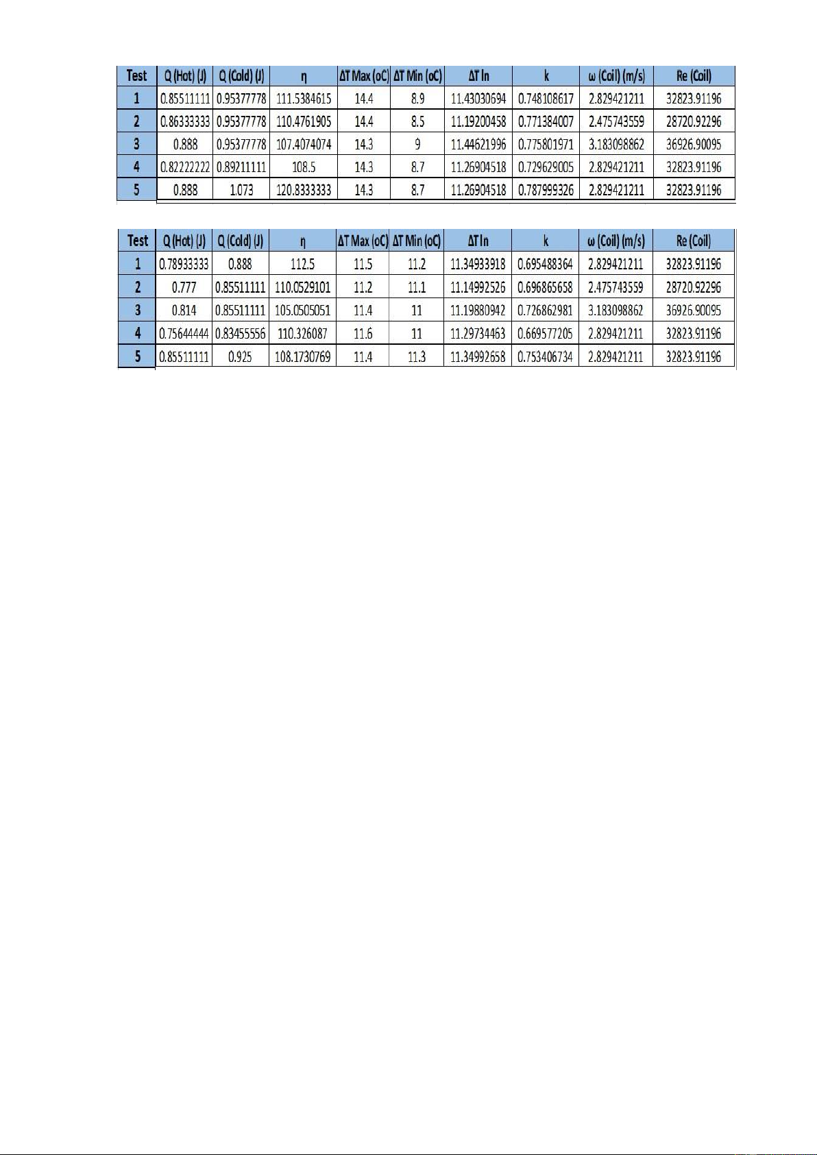
E2 (helical-coil heat exchanger) in PARALLEL flow: lOMoARcPSD| 36667950
E2 (helical-coil heat exchanger) in COUNTER flow: lOMoARcPSD| 36667950