
Basic Statistics Report - Ngôn ngữ anh | Học viện Tòa án

Variability is a measure of the dispersion or spread of a set of data, allowing forcomparison between different datasets. There are four primary methods forcharacterizing variability in a dataset: Range, Interquartile range, Variance, andStandard deviation (Frost, 2018). Tài liệu giúp bạn tham khảo, ôn tập và đạt kết quả cao. Mời bạn đọc đón xem!

Student name: Khanh Ha Quach
Student ID: 221117014
Basic statistics 1 – Final assignment
Assignment 1: Variability of Dataset
Variability is a measure of the dispersion or spread of a set of data, allowing for
comparison between different datasets. There are four primary methods for
characterizing variability in a dataset: Range, Interquartile range, Variance, and
Standard deviation (Frost, 2018).
The represents the difference between the largest and smallest values in arange
dataset. For instance, consider an MBA class with 5 students who received
grades of 6, 7, 8, 9, and 10 on their final exam. The range of grades in the class
is from 6 to 10. It is worth noting that an outlier, either extremely high or low,
can greatly impact the range, even if it is not representative of the majority of
the data. The size of the dataset also affects the range. With a smaller sample
size, it is less likely to observe extreme values, while a larger sample size
increases the chances of such values being present. Hence, when comparing
variability using the range, it is important to ensure that the sample sizes are
similar.
The is similar to the range but only encompasses theinterquartile range
middle 50% of the data. This is accomplished by dividing the dataset into
quarters, referred to as quartiles, denoted as Q1, Q2, and Q3. Q1 represents the
lowest 25% of the data, while Q4 represents the highest 25% of the data. The
interquartile range encompasses the values between Q1 and Q3, which is the
middle 50% of the data.
Variance provides a general sense of how spread out a dataset is by comparing
each value to the mean of the dataset, including all values in the calculation. A
low variance means the data is tightly clustered, while a high variance indicates
a more dispersed dataset. Variance is often used in the calculation of the
standard deviation, and it can be calculated as either population variance or
sample variance.
Population variance
The formula for the variance of an entire population is the following:
In the equation, σ is the population for the variance, μ is the
2
parameter
parameter for the population mean, and N is the number of data points, which
should include the entire population.
Sample variance
Sample variance is calculated when a sample is used to estimate the variance for
a population, as using the population variance with sample data tends to
underestimate the variability. However, entire population is usually impossible
to be measured, statisticians use the equation for sample variances much more
frequently.
In the equation, s is the sample variance, and M is the sample mean. N-1 in the
2
denominator corrects for the tendency of a sample to underestimate the
population variance.
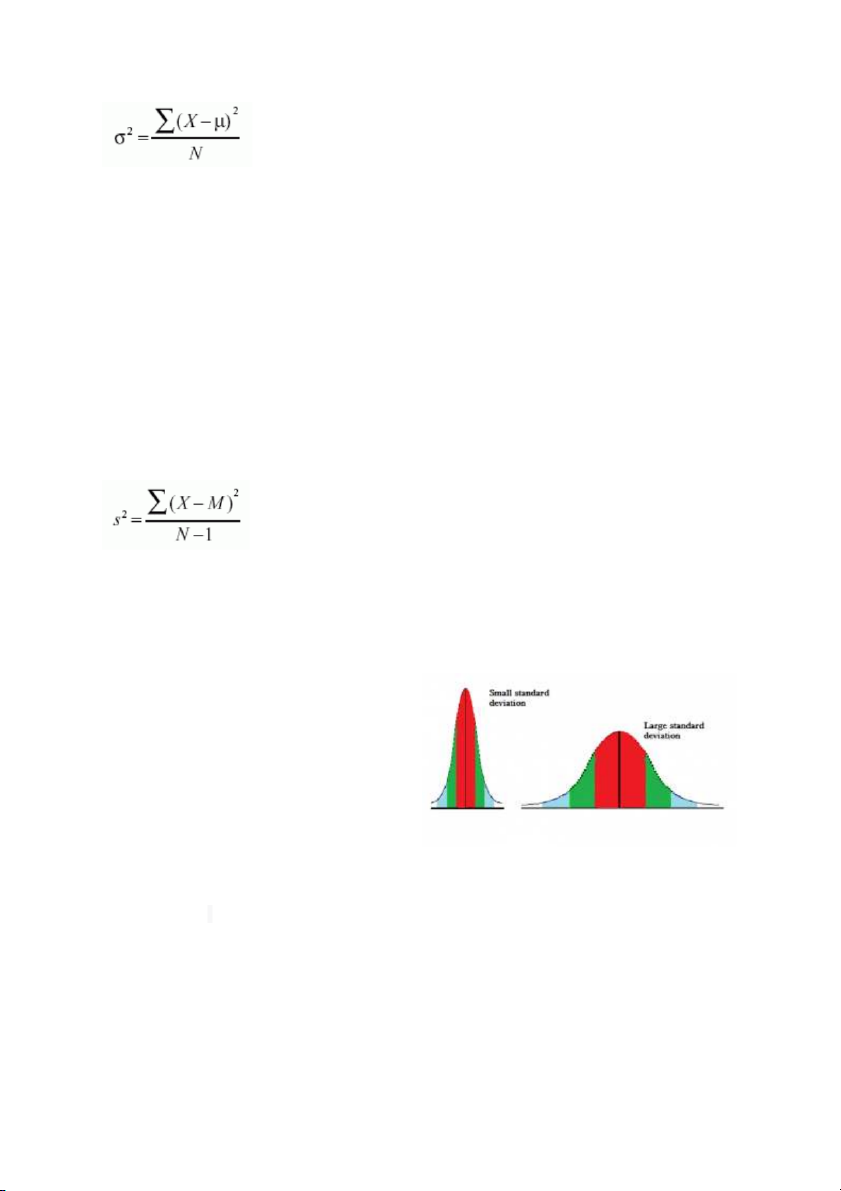
The standard deviation (SD) provides
information on the tightness of
clustering of the data around the
mean. A small standard deviation
indicates that the data points are
closely clustered around the mean,
resulting in a tall bell-shaped
distribution. Conversely, a large
standard deviation suggests that the data is more spread out. Additionally, it is
simply the square root of the variance, with the variance being expressed in
squared units.
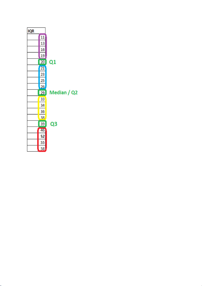
Taking example of a data set with 19 values (11;
13; 16; 19;…; 58) as following:
Mean = 31.26
Range = 58 – 11 = 47
Q1 Q3 = 20; Q2/ Median = 29; = 39
Interquartile range = Q3 – Q1 = 39 – 20 = 19
(Sample) Variance = [(11 31.26)^2 + (13
31.26)^2 + + (58 31.26)^2] / (19-1) =
197.98
Standard deviation = Squared root (variance)
= 14.07
Assignment 2: Correlation between Two Variables
A between variables signifies that a change in the value of onecorrelation
variable is associated with a corresponding change in the value of the other
variable. The correlation coefficient is a measure of the direction and magnitude
of this relationship, indicating the strength of the association between the two
variables:
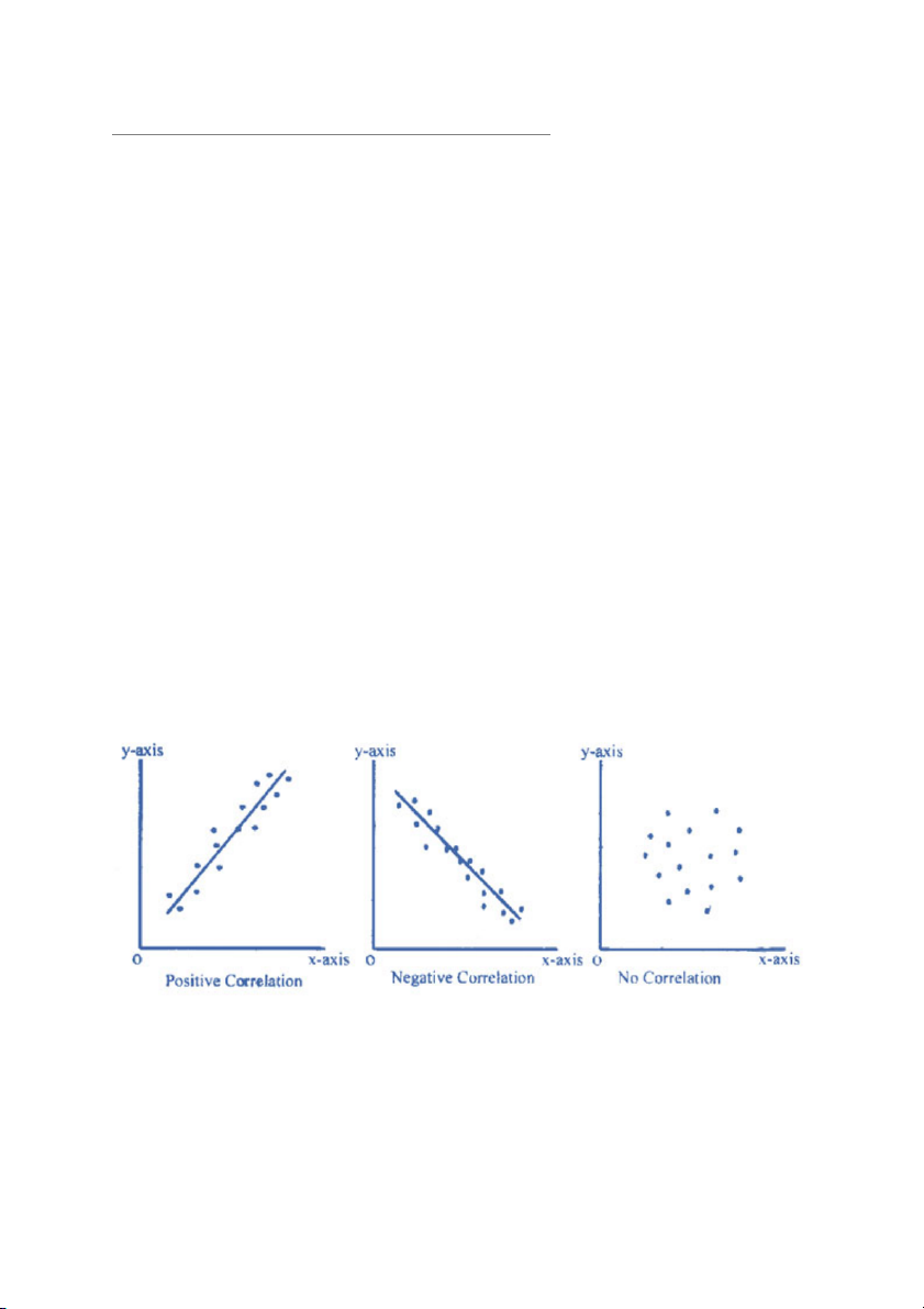
o A indicates that as one variable increases thepositive correlation
other variable tends to increase.
o A indicates that as one variable increases, therecorrelation near zero
is no tendency in the other variable to either increase or decrease.
o A indicates that as one variable increases thenegative correlation
other variable tends to decrease.
The correlation coefficient ranges from -1 to 1, with -1 and 1 indicating a
perfect linear relationship. When the correlation coefficient is -1, a change in
one variable is accompanied by a perfectly consistent change in the opposite
direction for the other variable. Conversely, when the correlation coefficient is
1, a change in one variable is accompanied by a perfectly consistent change in
the same direction for the other variable. These values indicate a strong, linear
relationship between the two variables.
Correlation does not mean Causation.
It is important to distinguish between correlation and causality. The mere fact
that two variables are correlated does not necessarily mean that one variable
causes changes in the other. Correlation only assesses the relationship between
variables and does not infer causality. There may be other factors that contribute
to the relationship between the variables, and it is possible that the correlation is
coincidental or due to some other underlying cause. Thus, while causation may
explain the correlation, it is not the only possible explanation and must be
established through additional evidence and analysis.
The correlation coefficient that indicates the strength of the relationship
between two variables can be found using the following formula:
Where:
r
xy
the correlation coefficient of the linear relationship between the
variables x and y
x
i
– the values of the x-variable in a sample
x – the mean of the values of the x-variable
y
i
– the values of the y-variable in a sample
ȳ – the mean of the values of the y-variable
Example of Correlation ( )Correlation
John, an investor, wants to evaluate the relationship between the stock of Apple
Inc. and the S&P 500 index, which is the primary focus of his portfolio. To do
so, he has gathered five years of price data for both. He wants to make sure that
adding Apple stock won't increase the systematic risk of his portfolio. John
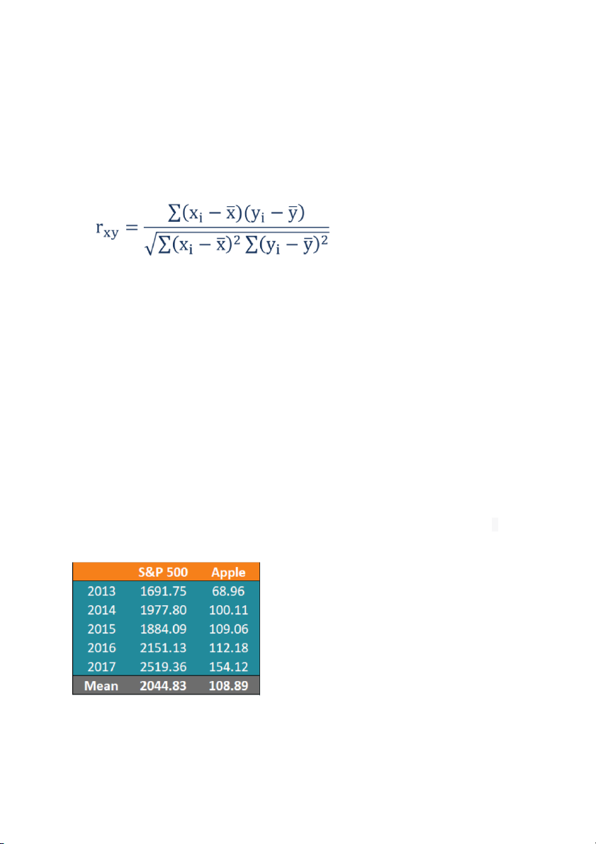
gathers the following prices for the last five years:
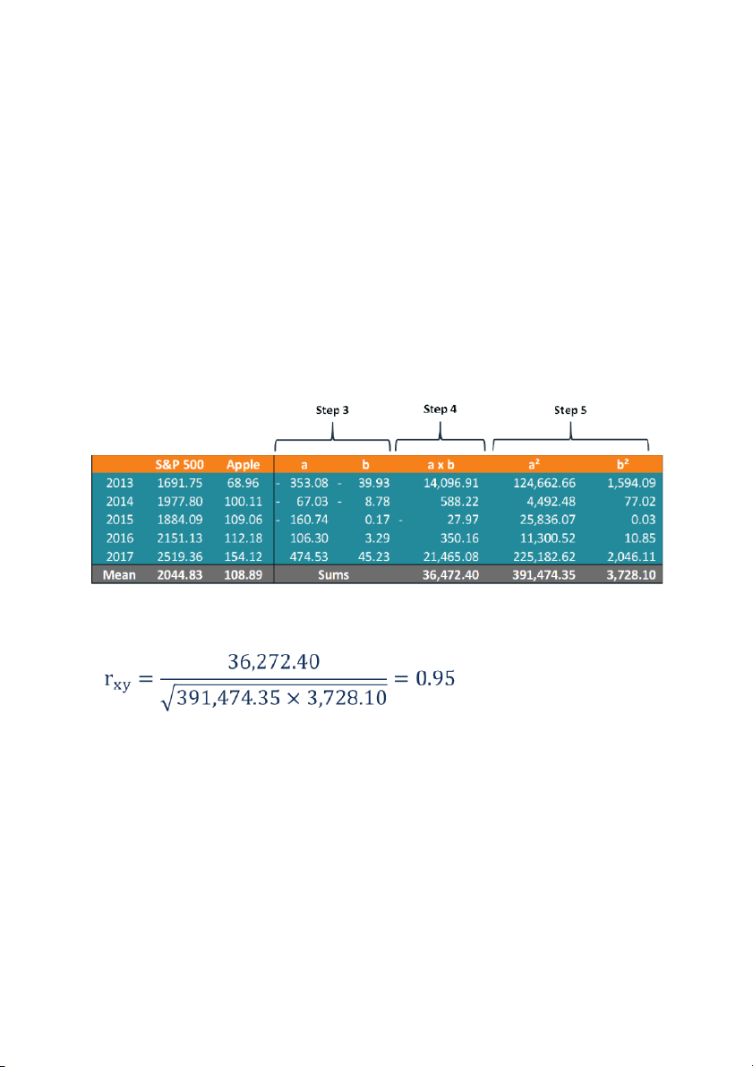
First, John calculates the average prices of each security for the given periods.
Then the other values are calculated in the following table:
Step 3:
Third column (a = S&P 500 value – S&P 500 mean value)
2044.83 – 1691.75 = -353.08
Forth column (b = Apple value – Apple mean value)
68.96 – 108.89 = - 39.93
Step 4: Multiply value of a and b from the same row
(-353.08) x (-39.93) = 14,096.91
Step 5: Square each value of a and b
Using the obtained numbers, John can calculate the coefficient:
The results show a strong positive correlation between the two, indicating that
their prices tend to move in tandem. Hence, incorporating Apple into his
portfolio would increase its systematic risk.
Assignment 3: Conditional probability
The conditional probability of an event B is the probability that the event will
occur given the knowledge that an event A has already occurred.
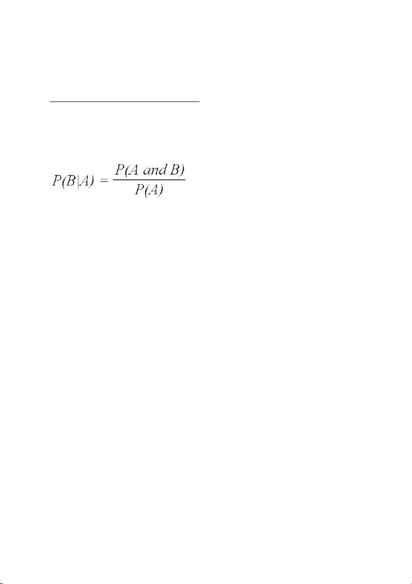
This probability is written P(B|A), notation for the probability of B given A:
Note: This expression is only valid when P(A) is greater than 0.
Dependent events can be contrasted with independent events. A dependent
event is one where the probability of the event occurring is affected by whether
another event occurred. If events A and B are independent, then the probability
of event B taking place given that event A has occurred is equal to the
standalone probability of event B, represented as P(B).
In contrast, an is one where the probability of the eventindependent event
occurring is the same regardless of the outcome of any other events. Then the
likelihood of both events happening together (the intersection of A and B) is
calculated as the product of the probability of event A and the conditional
probability of event B given event A. In other words, P(A and B) is equal to
P(A) multiplied by the probability of event B given that event A has already
occurred, represented as P(B|A).
Examples of conditional probability
1. In a card game where the goal is to draw two cards of the same suit, there
are 13 cards of each suit among the total of 52 cards. If the first card
drawn is a heart, then there are 12 hearts left in the deck of 51 cards
remaining. This means that the probability of drawing a second heart
given that the first card was a heart, P(Draw second heart | First card a
heart), is equal to 12/51.
2. The probability of an applicant getting accepted into college and being
offered dormitory housing can be calculated as follows: If the applicant
has an 80% chance of being accepted, and it is known that only 60% of
the accepted students will receive dormitory housing, the probability of
the applicant being accepted and receiving dormitory housing can be
determined by multiplying the two probabilities. The formula for this
would be P(Accepted and Dormitory Housing) = P(Dormitory Housing|
Accepted)P(Accepted) = (0.60) * (0.80) = 0.48.
3. To calculate the chance of multiple events happening at the same time,
the interdependence of all previous events must be taken into account. If
we have three events, A, B, and C, the probability of all three happening
simultaneously can be expressed as P(A and B and C) = P(A) * P(B given
A has occurred) * P(C given both A and B have occurred).
To calculate the probability of the college applicant being accepted, receiving
dormitory housing, and having no roommates, the conditional probabilities of
acceptance, receiving dormitory housing, and having roommates must be taken
into account. Based on the given information, the individual has a 0.80
probability of being accepted and a 0.60 probability of receiving dormitory
housing. Out of those accepted students who will receive housing, the
probability of having at least one roommate is 0.80. The resulting probability
can be calculated as:
P(Accepted and Dormitory Housing and No Roommates)
= P(Accepted) * P(Dormitory Housing|Accepted) * P(No Roomates|Dormitory
Housing and Accepted)
= (0.80)*(0.60)*(0.20) = 0.096.
Thus, the student has about a 9.6 % chance of receiving a single room at the
college.
Bayes’s formula:
The relationship between P(A|B) and P(B|A) can be established through Bayes'
theorem, named after Thomas Bayes, an 18th-century clergyman. Bayes'
theorem enables the calculation of reverse probabilities, allowing the estimation
of the likelihood of an event occurring, given that another related event has
taken place. In essence, Bayes' theorem states that the probability of event B is
the sum of the conditional probabilities of event B, given that event A has
happened or not.
Bayes's formula is defined as follows:
Where:
P(A|B) – the probability of event A occurring, given event B has occurred
P(B|A) – the probability of event B occurring, given event A has occurred
P(A) – the probability of event A
P(B) – the probability of event B
Example of Bayes’ Theorem (Bayes’ Theorem)
The study of publicly-traded companies showed that 60% of the companies with
a stock price increase of over 5% in the last three years changed their CEO
during that time frame. Meanwhile, only 35% of companies without such a
stock price increase replaced their CEO. Given the likelihood of a stock price
growth of over 5% is 4%, determine the probability that a company whose CEO
has been fired will experience a stock price increase of over 5%.
Event A: Stock price increases by 5% and Event B: CEO is replaced
P(A) – the probability that the stock price increases by 5%
P(B) – the probability that the CEO is replaced
P(A|B) – the probability of the stock price increases by 5% given that the
CEO has been replaced
P(B|A) the probability of the CEO replacement given the stock price
has increased by 5%.
Using the Bayes’ theorem, we can find the required probability:
Thus, the probability that the shares of a company that replaces its CEO will
grow by more than 5% is 6.67%.
References
Bayes’ Theorem (no date) Corporate Finance Institute. Available at:
https://corporatefinanceinstitute.com/resources/data-science/bayes-theorem/
(Accessed: 4 February 2023).
Correlation (no date) Corporate Finance Institute. Available at:
https://corporatefinanceinstitute.com/resources/data-science/correlation/
(Accessed: 4 February 2023).
Frost, J. (2018) ‘Measures of Variability: Range, Interquartile Range, Variance,
and Standard Deviation’, Statistics By Jim, 2 March. Available at:
http://statisticsbyjim.com/basics/variability-range-interquartile-variance-
standard-deviation/ (Accessed: 4 February 2023).

| 1/10

Preview text:

Student name: Khanh Ha Quach Student ID: 221117014
Basic statistics 1 – Final assignment
Assignment 1: Variability of Dataset
Variability is a measure of the dispersion or spread of a set of data, allowing for
comparison between different datasets. There are four primary methods for
characterizing variability in a dataset: Range, Interquartile range, Variance, and
Standard deviation (Frost, 2018).
The range represents the difference between the largest and smallest values in a
dataset. For instance, consider an MBA class with 5 students who received
grades of 6, 7, 8, 9, and 10 on their final exam. The range of grades in the class
is from 6 to 10. It is worth noting that an outlier, either extremely high or low,
can greatly impact the range, even if it is not representative of the majority of
the data. The size of the dataset also affects the range. With a smaller sample
size, it is less likely to observe extreme values, while a larger sample size
increases the chances of such values being present. Hence, when comparing
variability using the range, it is important to ensure that the sample sizes are similar.
The interquartile range is similar to the range but only encompasses the
middle 50% of the data. This is accomplished by dividing the dataset into
quarters, referred to as quartiles, denoted as Q1, Q2, and Q3. Q1 represents the
lowest 25% of the data, while Q4 represents the highest 25% of the data. The
interquartile range encompasses the values between Q1 and Q3, which is the middle 50% of the data.
Variance provides a general sense of how spread out a dataset is by comparing
each value to the mean of the dataset, including all values in the calculation. A
low variance means the data is tightly clustered, while a high variance indicates
a more dispersed dataset. Variance is often used in the calculation of the
standard deviation, and it can be calculated as either population variance or sample variance. Population variance
The formula for the variance of an entire population is the following:
In the equation, σ2 is the population parameter for the variance, μ is the
parameter for the population mean, and N is the number of data points, which
should include the entire population. Sample variance
Sample variance is calculated when a sample is used to estimate the variance for
a population, as using the population variance with sample data tends to
underestimate the variability. However, entire population is usually impossible
to be measured, statisticians use the equation for sample variances much more frequently.
In the equation, s2 is the sample variance, and M is the sample mean. N-1 in the
denominator corrects for the tendency of a sample to underestimate the population variance.
The standard deviation (SD) provides
information on the tightness of
clustering of the data around the
mean. A small standard deviation
indicates that the data points are
closely clustered around the mean,
resulting in a tall bell-shaped
distribution. Conversely, a large
standard deviation suggests that the data is more spread out. Additionally, it is
simply the square root of the variance, with the variance being expressed in squared units.
Taking example of a data set with 19 values (11;
13; 16; 19;…; 58) as following: Mean = 31.26 Range = 58 – 11 = 47
Q1 = 20; Q2/ Median Q3 = 29; = 39
Interquartile range = Q3 – Q1 = 39 – 20 = 19
(Sample) Variance = [(11 – 31.26)^2 + (13 –
31.26)^2 + … + (58 – 31.26)^2] / (19-1) = 197.98
Standard deviation = Squared root (variance) = 14.07
Assignment 2: Correlation between Two Variables
A correlation between variables signifies that a change in the value of one
variable is associated with a corresponding change in the value of the other
variable. The correlation coefficient is a measure of the direction and magnitude
of this relationship, indicating the strength of the association between the two variables:
o A positive correlation indicates that as one variable increases the
other variable tends to increase.
o A correlation near zero indicates that as one variable increases, there
is no tendency in the other variable to either increase or decrease.
o A negative correlation indicates that as one variable increases the
other variable tends to decrease.
The correlation coefficient ranges from -1 to 1, with -1 and 1 indicating a
perfect linear relationship. When the correlation coefficient is -1, a change in
one variable is accompanied by a perfectly consistent change in the opposite
direction for the other variable. Conversely, when the correlation coefficient is
1, a change in one variable is accompanied by a perfectly consistent change in
the same direction for the other variable. These values indicate a strong, linear
relationship between the two variables.
Correlation does not mean Causation.
It is important to distinguish between correlation and causality. The mere fact
that two variables are correlated does not necessarily mean that one variable
causes changes in the other. Correlation only assesses the relationship between
variables and does not infer causality. There may be other factors that contribute
to the relationship between the variables, and it is possible that the correlation is
coincidental or due to some other underlying cause. Thus, while causation may
explain the correlation, it is not the only possible explanation and must be
established through additional evidence and analysis.
The correlation coefficient that indicates the strength of the relationship
between two variables can be found using the following formula: Where:
rxy – the correlation coefficient of the linear relationship between the variables x and y
xi – the values of the x-variable in a sample
x – the mean of the values of the x-variable
yi – the values of the y-variable in a sample
ȳ – the mean of the values of the y-variable
Example of Correlation (Correlation)
John, an investor, wants to evaluate the relationship between the stock of Apple
Inc. and the S&P 500 index, which is the primary focus of his portfolio. To do
so, he has gathered five years of price data for both. He wants to make sure that
adding Apple stock won't increase the systematic risk of his portfolio. John
gathers the following prices for the last five years:
First, John calculates the average prices of each security for the given periods.
Then the other values are calculated in the following table: Step 3:
Third column (a = S&P 500 value – S&P 500 mean value) 2044.83 – 1691.75 = -353.08
Forth column (b = Apple value – Apple mean value) 68.96 – 108.89 = - 39.93
Step 4: Multiply value of a and b from the same row
(-353.08) x (-39.93) = 14,096.91
Step 5: Square each value of a and b
Using the obtained numbers, John can calculate the coefficient:
The results show a strong positive correlation between the two, indicating that
their prices tend to move in tandem. Hence, incorporating Apple into his
portfolio would increase its systematic risk.
Assignment 3: Conditional probability
The conditional probability of an event B is the probability that the event will
occur given the knowledge that an event A has already occurred.
This probability is written P(B|A), notation for the probability of B given A:
Note: This expression is only valid when P(A) is greater than 0.
Dependent events can be contrasted with independent events. A dependent
event is one where the probability of the event occurring is affected by whether
another event occurred. If events A and B are independent, then the probability
of event B taking place given that event A has occurred is equal to the
standalone probability of event B, represented as P(B).
In contrast, an independent event is one where the probability of the event
occurring is the same regardless of the outcome of any other events. Then the
likelihood of both events happening together (the intersection of A and B) is
calculated as the product of the probability of event A and the conditional
probability of event B given event A. In other words, P(A and B) is equal to
P(A) multiplied by the probability of event B given that event A has already
occurred, represented as P(B|A).
Examples of conditional probability
1. In a card game where the goal is to draw two cards of the same suit, there
are 13 cards of each suit among the total of 52 cards. If the first card
drawn is a heart, then there are 12 hearts left in the deck of 51 cards
remaining. This means that the probability of drawing a second heart
given that the first card was a heart, P(Draw second heart | First card a heart), is equal to 12/51.
2. The probability of an applicant getting accepted into college and being
offered dormitory housing can be calculated as follows: If the applicant
has an 80% chance of being accepted, and it is known that only 60% of
the accepted students will receive dormitory housing, the probability of
the applicant being accepted and receiving dormitory housing can be
determined by multiplying the two probabilities. The formula for this
would be P(Accepted and Dormitory Housing) = P(Dormitory Housing|
Accepted)P(Accepted) = (0.60) * (0.80) = 0.48.
3. To calculate the chance of multiple events happening at the same time,
the interdependence of all previous events must be taken into account. If
we have three events, A, B, and C, the probability of all three happening
simultaneously can be expressed as P(A and B and C) = P(A) * P(B given
A has occurred) * P(C given both A and B have occurred).
To calculate the probability of the college applicant being accepted, receiving
dormitory housing, and having no roommates, the conditional probabilities of
acceptance, receiving dormitory housing, and having roommates must be taken
into account. Based on the given information, the individual has a 0.80
probability of being accepted and a 0.60 probability of receiving dormitory
housing. Out of those accepted students who will receive housing, the
probability of having at least one roommate is 0.80. The resulting probability can be calculated as:
P(Accepted and Dormitory Housing and No Roommates)
= P(Accepted) * P(Dormitory Housing|Accepted) * P(No Roomates|Dormitory Housing and Accepted)
= (0.80)*(0.60)*(0.20) = 0.096.
Thus, the student has about a 9.6 % chance of receiving a single room at the college. Bayes’s formula:
The relationship between P(A|B) and P(B|A) can be established through Bayes'
theorem, named after Thomas Bayes, an 18th-century clergyman. Bayes'
theorem enables the calculation of reverse probabilities, allowing the estimation
of the likelihood of an event occurring, given that another related event has
taken place. In essence, Bayes' theorem states that the probability of event B is
the sum of the conditional probabilities of event B, given that event A has happened or not.
Bayes's formula is defined as follows: Where:
 P(A|B) – the probability of event A occurring, given event B has occurred
 P(B|A) – the probability of event B occurring, given event A has occurred
 P(A) – the probability of event A
 P(B) – the probability of event B
Example of Bayes’ Theorem (Bayes’ Theorem)
The study of publicly-traded companies showed that 60% of the companies with
a stock price increase of over 5% in the last three years changed their CEO
during that time frame. Meanwhile, only 35% of companies without such a
stock price increase replaced their CEO. Given the likelihood of a stock price
growth of over 5% is 4%, determine the probability that a company whose CEO
has been fired will experience a stock price increase of over 5%.
Event A: Stock price increases by 5% and Event B: CEO is replaced
 P(A) – the probability that the stock price increases by 5%
 P(B) – the probability that the CEO is replaced
 P(A|B) – the probability of the stock price increases by 5% given that the CEO has been replaced
 P(B|A) – the probability of the CEO replacement given the stock price has increased by 5%.
Using the Bayes’ theorem, we can find the required probability:
Thus, the probability that the shares of a company that replaces its CEO will grow by more than 5% is 6.67%. References
Bayes’ Theorem (no date) Corporate Finance Institute. Available at:
https://corporatefinanceinstitute.com/resources/data-science/bayes-theorem/ (Accessed: 4 February 2023).
Correlation (no date) Corporate Finance Institute. Available at:
https://corporatefinanceinstitute.com/resources/data-science/correlation/ (Accessed: 4 February 2023).

Frost, J. (2018) ‘Measures of Variability: Range, Interquartile Range, Variance,
and Standard Deviation’, Statistics By Jim, 2 March. Available at:
http://statisticsbyjim.com/basics/variability-range-interquartile-variance-
standard-deviation/ (Accessed: 4 February 2023).