Chapter 1. Probability môn Xác suất thống kê| Trường Đại học Ngoại Thương

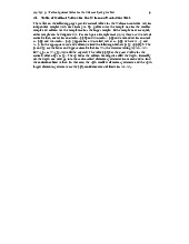
CHAPTER 1. PROBABILITY I. Solution Steps
+ Step 1: Define the events from the problem.
+ Step 2: Define the probabilities and conditional probabilities for the events defined in Step 1.
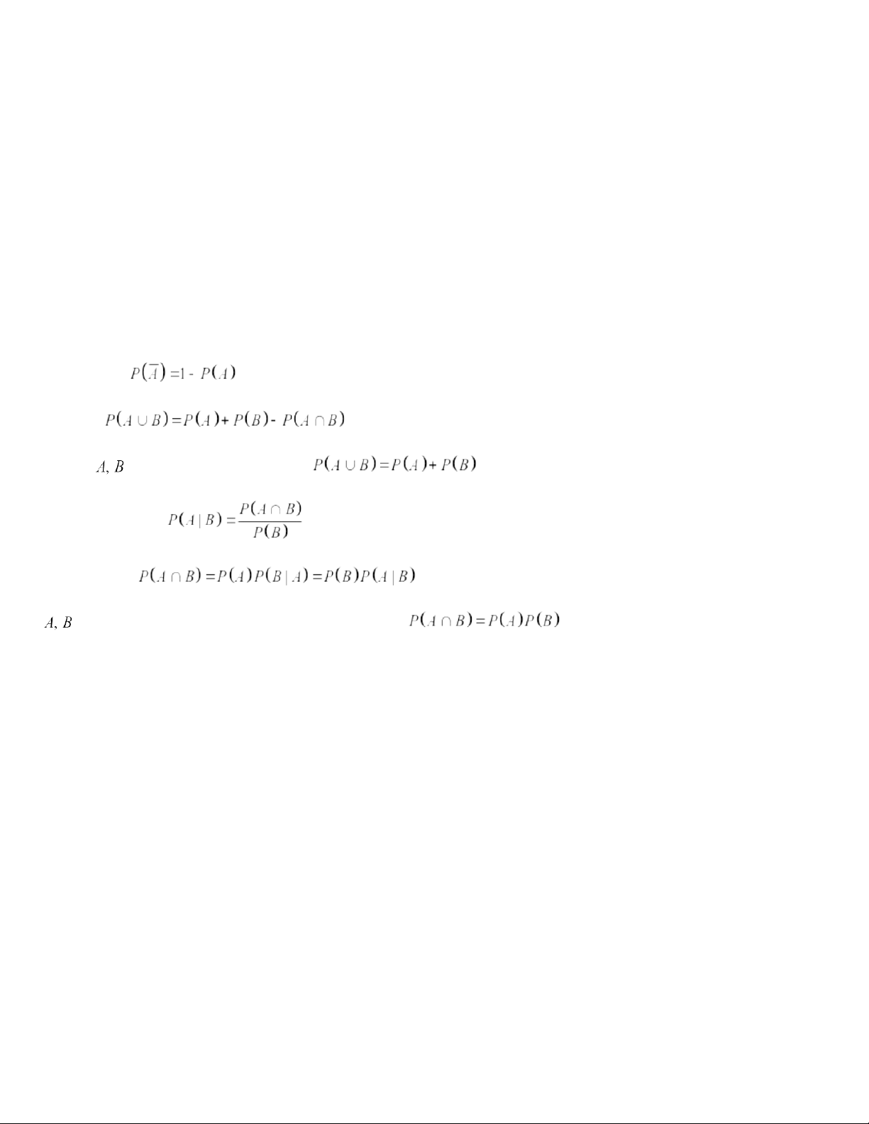
+ Step 3: Find the system of events which is both mutually exclusive and collectively exhaustive (compute the complement if needed). + Step 4: Apply the formula. II. Probability rules 1. Complement rule: . 2. Addition rule: . n particular, if are mutually exclusive, then . 3. Conditional probability: . 4. Multiplication rule: Events
are said to be statistically independent if and only if . 5. Total probability: Given the system of events
that are both mutually exclusive and collectively exhaustive, then or
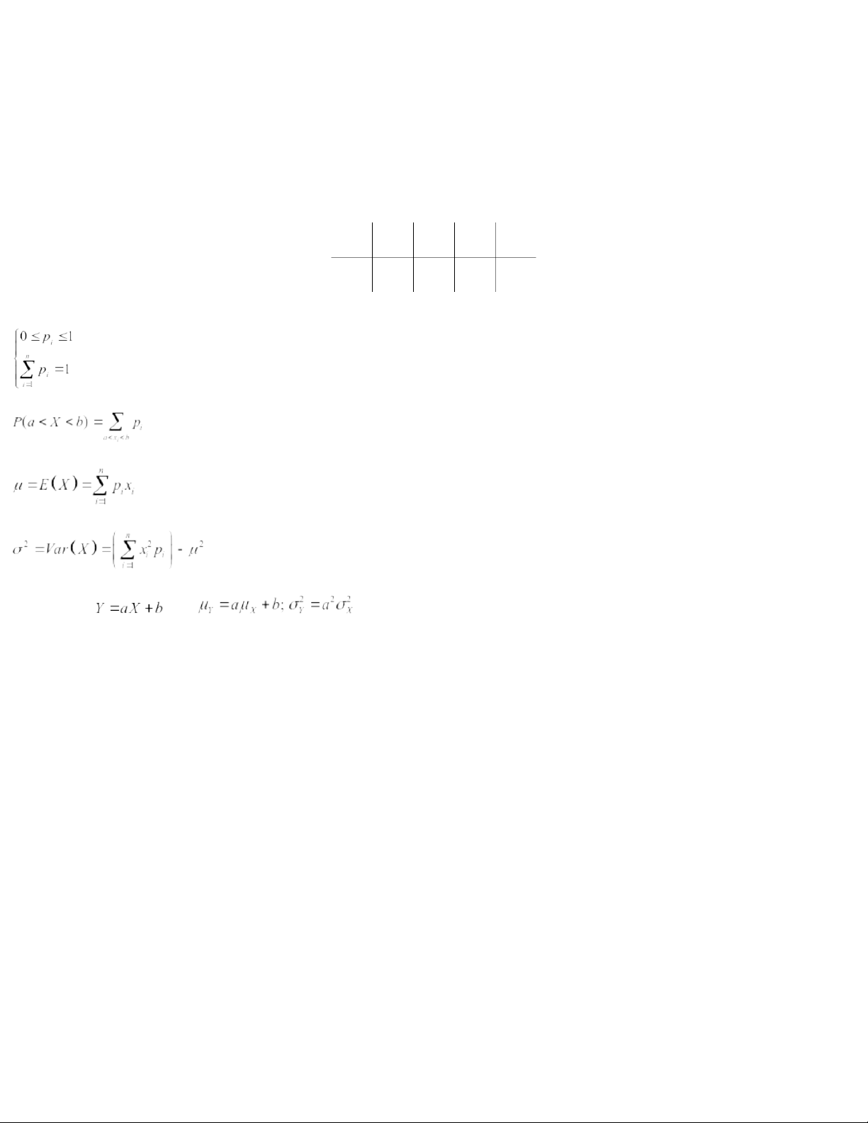
CHAPTER 2. DISCRETE RANDOM VARIABLES I. Distribution table Given the distribution table: Xx1x2….xn Pp1p2….pn Then 1. . 2. . 3. . 4. . n particular, if then .
II. Binomial Distribution Suppose that
a random experiment can result in two possible outcomes, “success” and “failure,”
and that p is the probability of a success in a single trial.
Let X be the the number of resulting successes in n independent trials.
The probability distribution of X is called binomial distribution.
III. Poisson Distribution
Let X be the number of occurrences in a given continuous interval (such as time, surface area, or length). Then the probability distribution
of X is called the Poisson distribution.
CHAPTER 3. CONTINUOUS RANDOM VARIABLES I. Density Function Given the density function
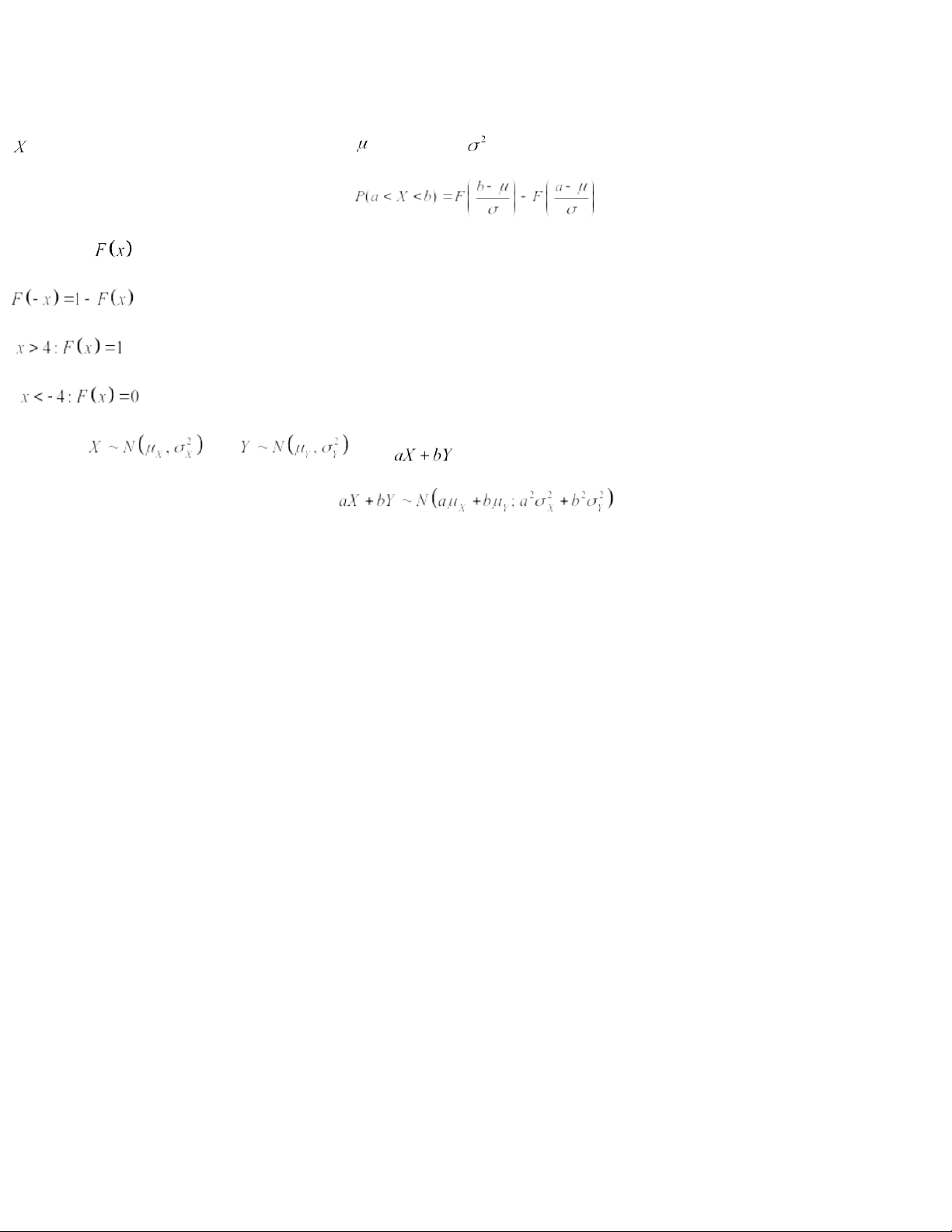
of a continuous random variable . Then i) ii) iii)t iv) v) vi) II. Normal Distribution f
follows the normal distribution with the mean and variance , then The values of
can be found in Appendix Table 1 with the notices ) . i) ii) Moreover, if and , then
also follows the normal distribution
CHAPTER 4. SAMPLING DISTRIBUTION Let the random variables
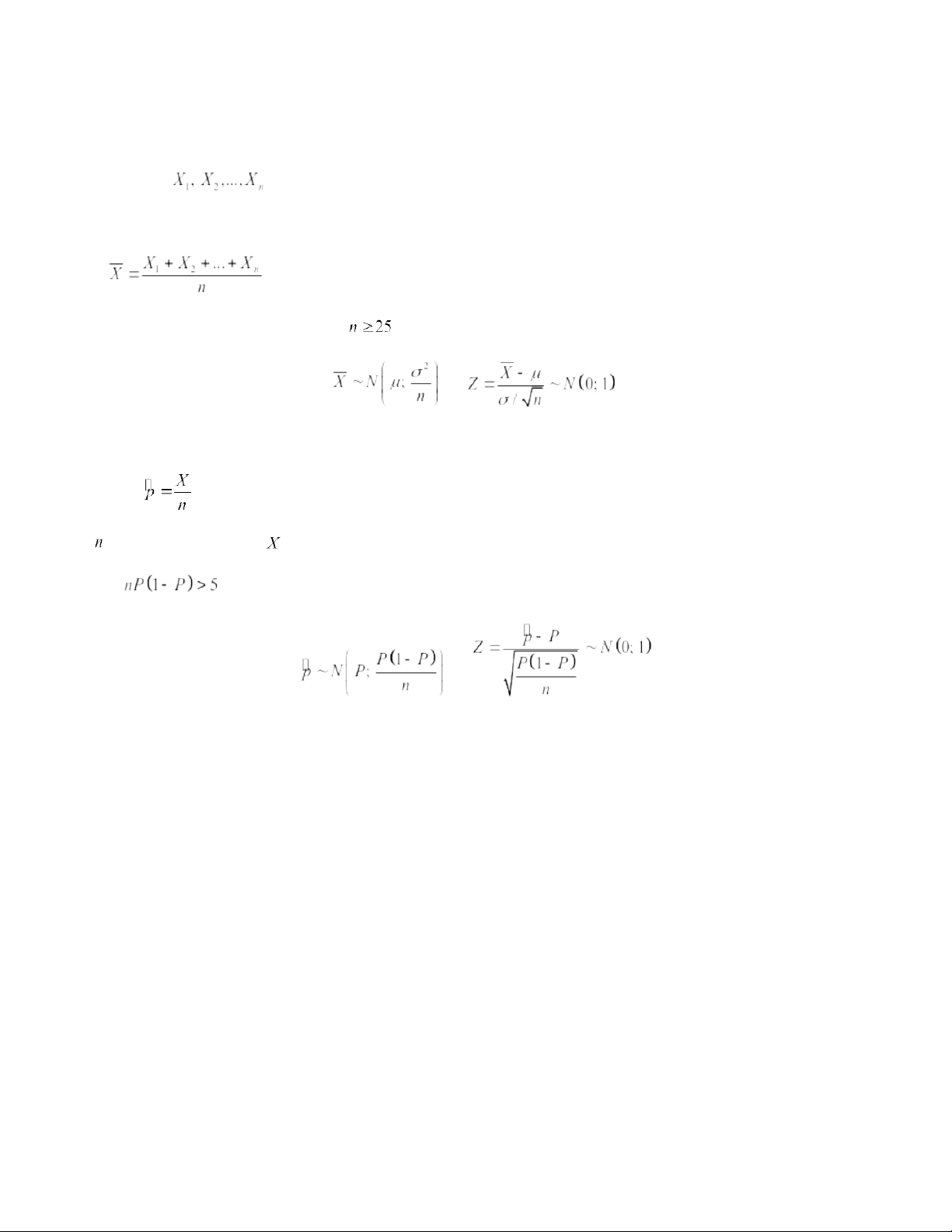
denote a random sample from a population. I. Sample mean Sample mean: .
If the parent population distribution is normal (or ) then or . II. Sample proportion Sample proportion: where is the sample size and
is the number of objects having the characteristic of interest. When n is large ( ), we have or III. Sample variance Sample variance: .
If the parent population distribution is normal then
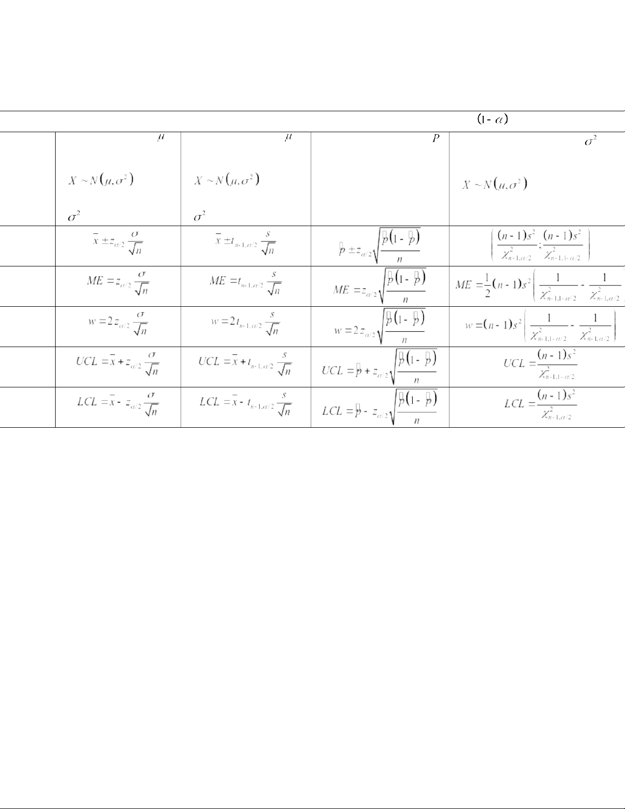
CHAPTER 5. CONFIDENCE INTERVAL ESTIMATION I. Formulas
Confidence Interval Estimation with the sample n and the confidence level Population mean Population mean Population proportion Population variance Given Given Given Estimation Given + n is large for + (or n is + (or n is + large) large) + is known + is unknown Confidenc e interval Margin of error Width Upper confidence limit Lower confidence limit II. Critical values
1. Critical values for the standard normal distribution: is a value such that Some critical values: Given the critical value
, we can determine the significant level (or confidence level ) by the following formula where
can be found in Appendix Table 1.
2. Critical values for the Student’s t distribution is a value such that The value
can be found in Appendix Table 8.
3. Critical values for the Chi-squared distribution is a value such that The value
can be found in Appendix Table 7a and 7b.
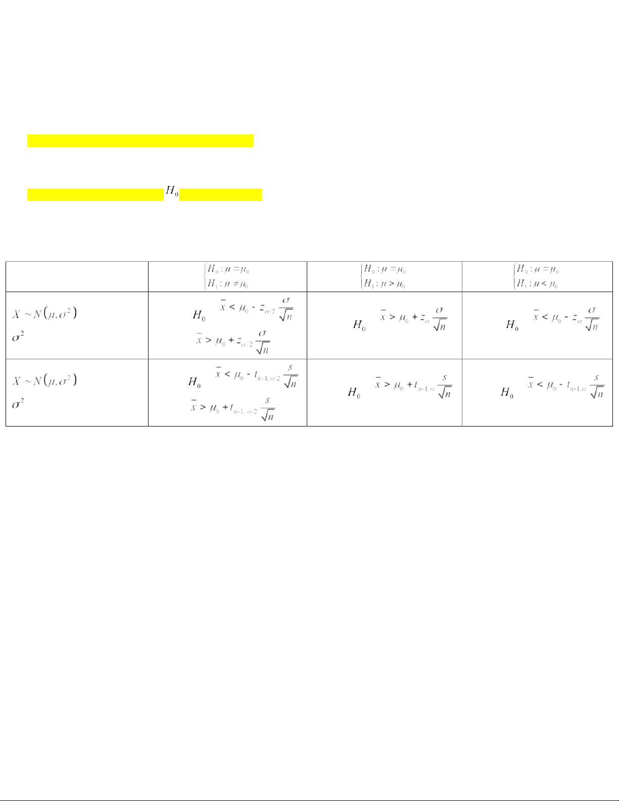
CHAPTER 6. HYPOTHESIS TESTS I. Solution steps
+ Step 1: State the null and alternative hypotheses.
+ Step 2: Summarize all information.
+ Step 3: Decision rule: reject if …… (Formula)
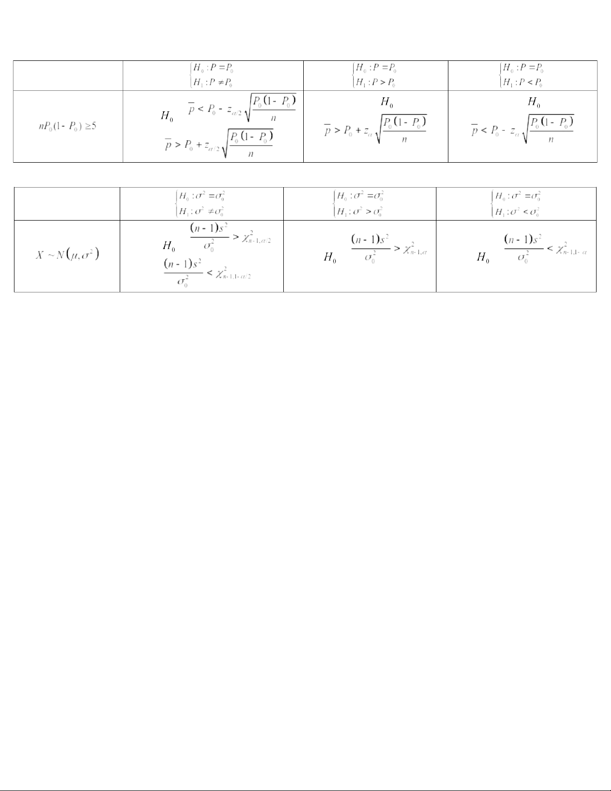
+ Step 4: Random sample => conclusion II. Decistion rule For population mean (or n is large) Reject if Reject if Reject if is known or (or n is large) Reject if Reject if Reject if is unknown or For population proportion Reject if Reject if Reject if or For population variance Reject if Reject if Reject if or