Chapter 11: Structure of Mass Nonvolatile Storage Systems | Môn Cơ sở hệ điều hành - Đại học Xây Dựng Hà Nội
The bulk of secondary storage for modern computers is provided by hard disk drives (HDDs) and nonvolatile memory (NVM) devices. Tài liệu được sưu tầm gồm 44 trang, giúp bạn ôn tập tốt hơn. Mời các bạn đón xem.
Môn: Cơ sở hệ điều hành 10 tài liệu
Trường: Trường Đại học Xây Dựng Hà Nội 540 tài liệu
Tác giả:


Preview text:
lOMoAR cPSD| 58933639 Mass-Storage CHAPTER Structure
In this chapter, we discuss how mass
storage—the nonvolatile storage system of
a computer—is structured. The main mass-
storage system in modern computers is
secondary storage, which is usually provided by hard disk drives (HDD) and
nonvolatile memory (NVM) devices. Some systems also have slower, larger, tertiary
storage, generally consisting of magnetic tape, optical disks, or even cloud storage.
Because the most common and important storage devices in modern computer
systems are HDDs and NVM devices, the bulk of this chapter is devoted to discussing
these two types of storage. We first describe their physical structure. We then consider
scheduling algorithms, which schedule the order of I/Os to maximize performance.
Next, we discuss device formatting and management of boot blocks, damaged blocks,
and swap space. Finally, we examine the structure of RAID systems.
There are many types of mass storage, and we use the general term nonvolatile
storage (NVS) or talk about storage “drives” when the discussion includes all types.
Particular devices, such as HDDs and NVM devices, are specified as appropriate. CHAPTER OBJECTIVES
• Describe the physical structures of various secondary storage devices and
the effect of a device’s structure on its uses.
• Explain the performance characteristics of mass-storage devices.
• Evaluate I/O scheduling algorithms.
• Discuss operating-system services provided for mass storage, including RAID. 11.1
Overview of Mass-Storage Structure
The bulk of secondary storage for modern computers is provided by hard disk drives
(HDDs) and nonvolatile memory (NVM) devices. In this section, 449 lOMoAR cPSD| 58933639 11.1
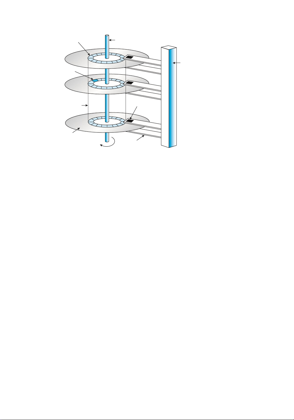
Overview of Mass-Storage Structure 450 track t spindle arm assembly sector s cylinder c read-write head platter arm rotation
Figure 11.1 HDD moving-head disk mechanism.
we describe the basic mechanisms of these devices and explain how operating systems translate
their physical properties to logical storage via address mapping. 11.1.1 Hard Disk Drives
Conceptually, HDDs are relatively simple (Figure 11.1). Each disk platter has a flat circular
shape, like a CD. Common platter diameters range from 1.8 to 3.5 inches. The two surfaces of
a platter are covered with a magnetic material. We store information by recording it
magnetically on the platters, and we read information by detecting the magnetic pattern on the platters.
A read–write head “flies” just above each surface of every platter. The heads are attached
to a disk arm that moves all the heads as a unit. The surface of a platter is logically divided
into circular tracks, which are subdivided into sectors. The set of tracks at a given arm position
make up a cylinder. There may be thousands of concentric cylinders in a disk drive, and each
track may contain hundreds of sectors. Each sector has a fixed size and is the smallest unit of
transfer. The sector size was commonly 512 bytes until around 2010. At that point, many
manufacturers start migrating to 4KB sectors. The storage capacity of common disk drives is
measured in gigabytes and terabytes. Adisk drive with the cover removed is shown in Figure 11.2.
Adisk drive motor spins it at high speed. Most drives rotate 60 to 250 times per second,
specified in terms of rotations per minute (RPM). Common drives spin at 5,400, 7,200, 10,000,
and 15,000 RPM. Some drives power down when not in use and spin up upon receiving an I/O
request. Rotation speed relates to transfer rates. The transfer rate is the rate at which data flow
between the drive and the computer. Another performance aspect, the positioning time, or
random-access time, consists of two parts: the time necessary to move the disk arm to the
desired cylinder, called the seek time, and the time necessary for the lOMoAR cPSD| 58933639 11.1
Overview of Mass-Storage Structure 451
Figure 11.2 A 3.5-inch HDD with cover removed.
desired sector to rotate to the disk head, called the rotational latency. Typical disks can transfer
tens to hundreds of megabytes of data per second, and they have seek times and rotational
latencies of several milliseconds. They increase performance by having DRAM buffers in the drive controller.
The disk head flies on an extremely thin cushion (measured in microns) of air or another
gas, such as helium, and there is a danger that the head will make contact with the disk surface.
Although the disk platters are coated with a thin protective layer, the head will sometimes
damage the magnetic surface. This accident is called a head crash. A head crash normally
cannot be repaired; the entire disk must be replaced, and the data on the disk are lost unless
they were backed up to other storage or RAID protected. (RAID is discussed in Section 11.8.)
HDDs are sealed units, and some chassis that hold HDDs allow their removal without
shutting down the system or storage chassis. This is helpful when a system needs more storage
than can be connected at a given time or when it is necessary to replace a bad drive with a
working one. Other types of storage media are also removable, including CDs, DVDs, and Blu- ray discs.
DISKTRANSFERRATES
As with many aspects of computing, published performance numbers for disks are not the
same as real-world performance numbers. Stated transfer rates are always higher
thaneffectivetransferrates, for example.The transfer rate may be the rate at which bits can be
read from the magnetic media by the disk head, but that is different from the rate at which
blocks are delivered to the operating system. 11.1.2 Nonvolatile Memory Devices lOMoAR cPSD| 58933639 11.1
Overview of Mass-Storage Structure 452
Nonvolatile memory (NVM) devices are growing in importance. Simply described, NVM
devices are electrical rather than mechanical. Most commonly, such a device is composed of a
controller and flash NAND die semiconductor chips, which are used to store data. Other NVM
technologies exist, like DRAM with battery backing so it doesn’t lose its contents, as well as
other semiconductor technology like 3D XPoint, but they are far less common and so are not discussed in this book. 11.1.2.1
Overview of Nonvolatile Memory Devices
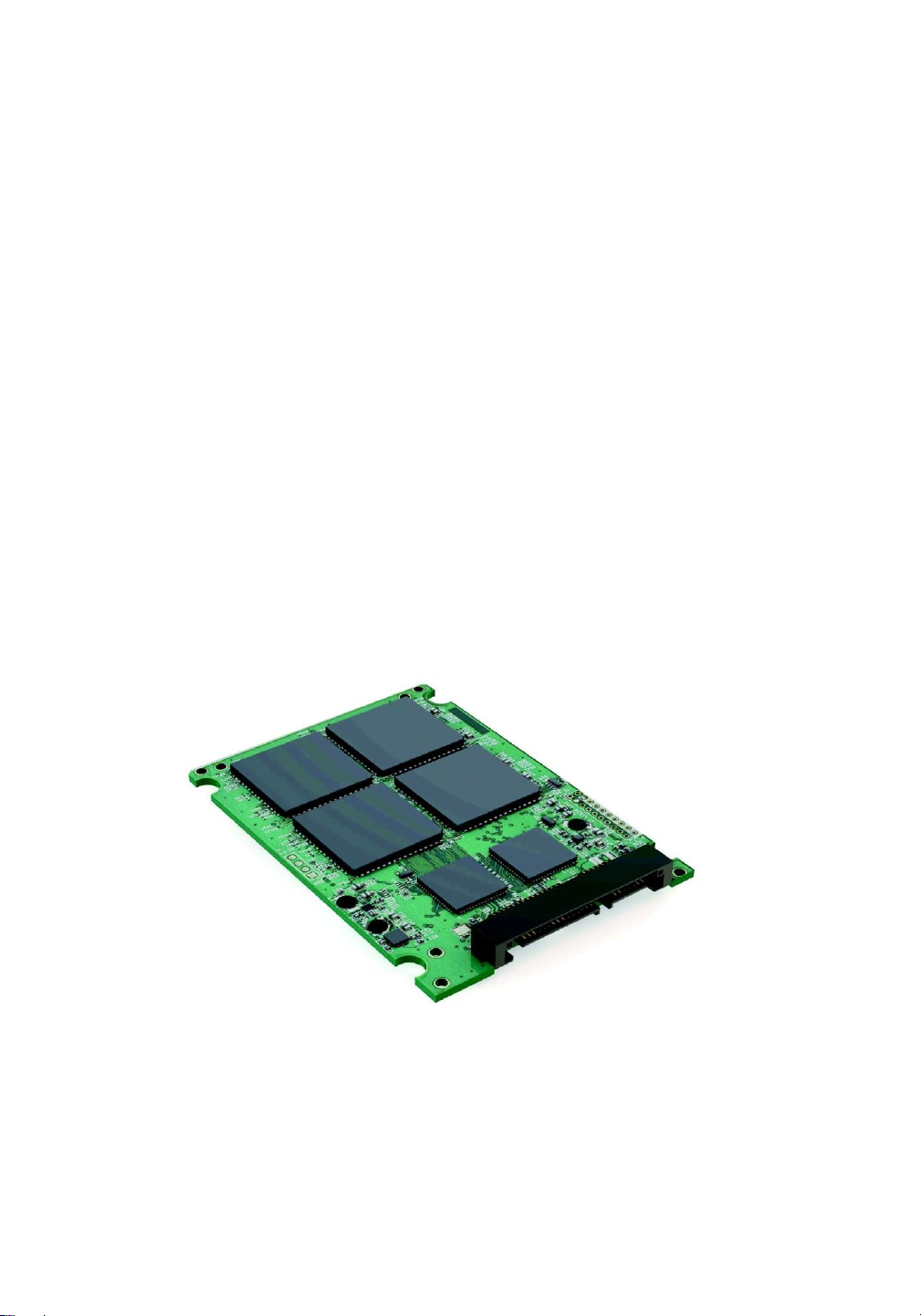
Flash-memory-based NVM is frequently used in a disk-drive-like container, in which case it is
called a solid-state disk (SSD) (Figure 11.3). In other instances, it takes the form of a USB drive
(also known as a thumb drive or flash drive) or a DRAM stick. It is also surfacemounted onto
motherboards as the main storage in devices like smartphones. In all forms, it acts and can be
treated in the same way. Our discussion of NVM devices focuses on this technology.
NVM devices can be more reliable than HDDs because they have no moving parts and can
be faster because they have no seek time or rotational latency. In addition, they consume less
power. On the negative side, they are more expensive per megabyte than traditional hard disks
and have less capacity than the larger hard disks. Over time, however, the capacity of NVM
devices has increased faster than HDD capacity, and their price has dropped more quickly, so
their use is increasing dramatically. In fact, SSDs and similar devices are now used in some
laptop computers to make them smaller, faster, and more energy-efficient.
Because NVM devices can be much faster than hard disk drives, standard bus interfaces can
cause a major limit on throughput. Some NVM devices are designed to connect directly to the
system bus (PCIe, for example). This technology is changing other traditional aspects of computer design as well.
Figure 11.3 A 3.5-inch SSD circuit board.
Some systems use it as a direct replacement for disk drives, while others use it as a new cache
tier, moving data among magnetic disks, NVM, and main memory to optimize performance.
NAND semiconductors have some characteristics that present their own storage and
reliability challenges. For example, they can be read and written in a “page” increment (similar
to a sector), but data cannot be overwritten— rather, the NAND cells have to be erased first. The lOMoAR cPSD| 58933639 11.1
Overview of Mass-Storage Structure 453
erasure, which occurs in a “block” increment that is several pages in size, takes much more
time than a read (the fastest operation) or a write (slower than read, but much faster than erase).
Helping the situation is that NVM flash devices are composed of many die, with many datapaths
to each die, so operations can happen in parallel (each using a datapath). NAND semiconductors
also deteriorate with every erase cycle, and after approximately 100,000 program-erase cycles
(the specific number varies depending on the medium), the cells no longer retain data. Because
of the write wear, and because there are no moving parts, NAND NVM lifespan is not measured
in years but in Drive Writes Per Day (DWPD). That measure is how many times the drive
capacity can be written per day before the drive fails. For example, a 1 TB NAND drive with a
5 DWPD rating is expected to have 5 TB per day written to it for the warranty period without failure.
These limitations have led to several ameliorating algorithms. Fortunately, they are usually
implemented in the NVM device controller and are not of concern to the operating system. The
operating system simply reads and writes logical blocks, and the device manages how that is
done. (Logical blocks are discussed in more detail in Section 11.1.5.) However, NVM devices
have performance variations based on their operating algorithms, so a brief discussion of what
the controller does is warranted. 11.1.2.2
NAND Flash Controller Algorithms
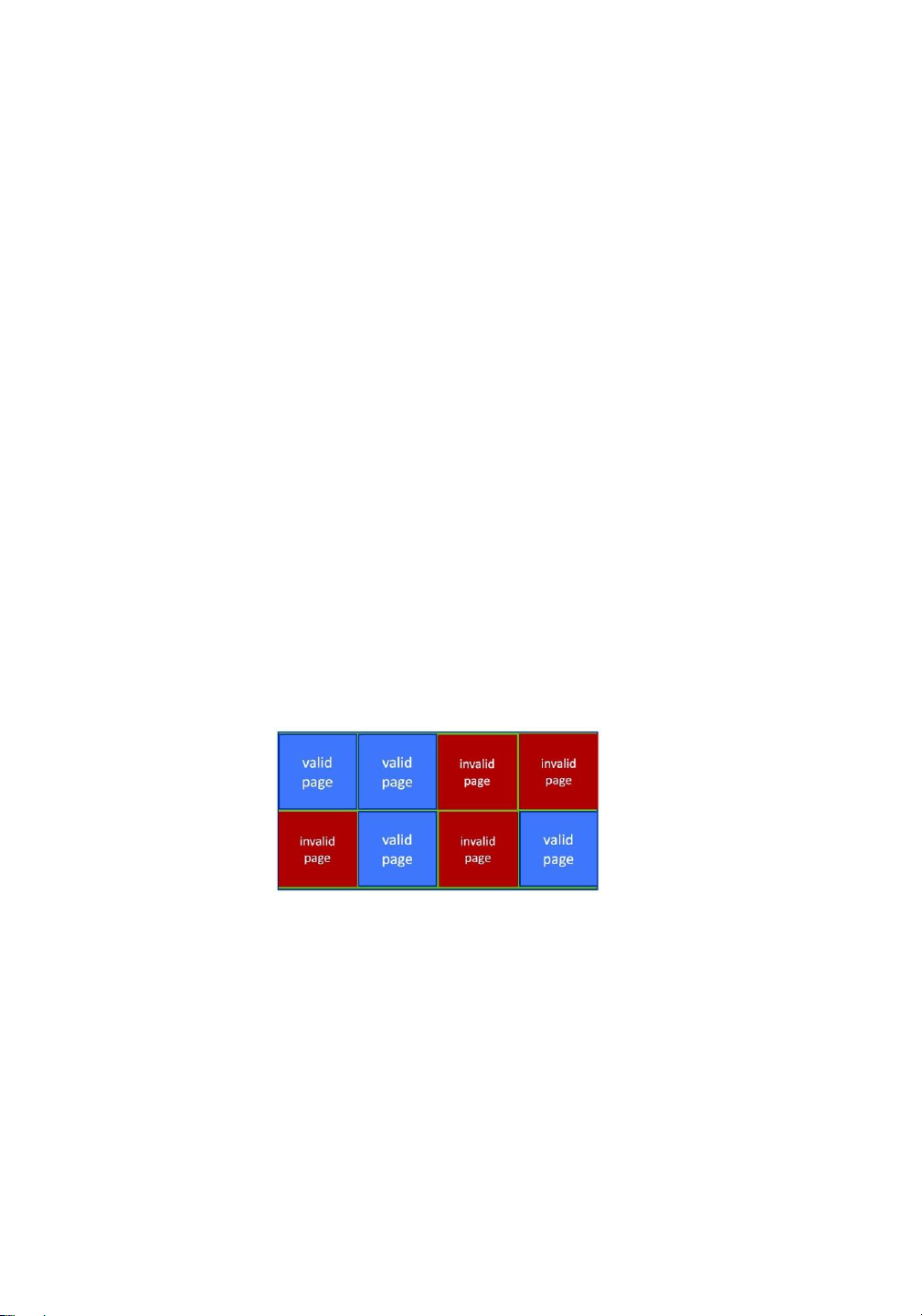
Because NAND semiconductors cannot be overwritten once written, there are usually pages
containing invalid data. Consider a file-system block, written once and then later written again.
If no erase has occurred in the meantime, the page first written has the old data, which are now
invalid, and the second page has the current, good version of the block. A NAND block
containing valid and invalid pages is shown in Figure 11.4. To track which logical blocks
contain valid data, the controller maintains a flas translation layer (FTL). This table maps
which physical pages contain currently valid logical blocks. It also
Figure 11.4 A NAND block with valid and invalid pages.
tracks physical block state—that is, which blocks contain only invalid pages and therefore can be erased.
Now consider a full SSD with a pending write request. Because the SSD is full, all pages
have been written to, but there might be a block that contains no valid data. In that case, the
write could wait for the erase to occur, and then the write could occur. But what if there are no
free blocks? There still could be some space available if individual pages are holding invalid
data. In that case, garbage collection could occur—good data could be copied to other
locations, freeing up blocks that could be erased and could then receive the writes. However,
where would the garbage collection store the good data? To solve this problem and lOMoAR cPSD| 58933639 11.1
Overview of Mass-Storage Structure 454
improve write performance, the NVM device uses overprovisioning. The device sets aside a
number of pages (frequently 20 percent of the total) as an area always available to write to.
Blocks that are totally invalid by garbage collection, or write operations invalidating older
versions of the data, are erased and placed in the over-provisioning space if the device is full or returned to the free pool.
The over-provisioning space can also help with wear leveling. If some blocks are erased
repeatedly, while others are not, the frequently erased blocks will wear out faster than the
others, and the entire device will have a shorter lifespan than it would if all the blocks wore
out concurrently. The controller tries to avoid that by using various algorithms to place data on
less-erased blocks so that subsequent erases will happen on those blocks rather than on the
more erased blocks, leveling the wear across the entire device.
In terms of data protection, like HDDs, NVM devices provide errorcorrecting codes, which
are calculated and stored along with the data during writing and read with the data to detect
errors and correct them if possible. (Error-correcting codes are discussed in Section 11.5.1.) If
a page frequently has correctible errors, the page might be marked as bad and not used in
subsequent writes. Generally, a single NVM device, like an HDD, can have a catastrophic failure
in which it corrupts or fails to reply to read or write requests. To allow data to be recoverable
in those instances, RAID protection is used. 11.1.3 Volatile Memory
It might seem odd to discuss volatile memory in a chapter on mass-storage structure, but it is
justifiable because DRAM is frequently used as a mass-storage device. Specifically, RAM drives
(which are known by many names, including RAM disks) act like secondary storage but are
created by device drivers that carve out a section of the system’s DRAM and present it to the
rest of the system as it if were a storage device. These “drives” can be used as raw block
devices, but more commonly, file systems are created on them for standard file operations.
Computers already have buffering and caching, so what is the purpose of yet another use
of DRAM for temporary data storage? After all, DRAM is volatile, and data on a RAM drive does
not survive a system crash, shutdown, or power down. Caches and buffers are allocated by the
programmer or operating system, whereas RAM drives allow the user (as well as the programmer) to place MAGNETICTAPES
Magnetic tape was used as an early secondary-storage medium. Although it is nonvolatile
and can hold large quantities of data, its access time is slow compared with that of main
memory and drives. In addition, random access to magnetic tape is about a thousand times
slower than random access to HDDs and about a hundred thousand times slower than random
access to SSDs so tapes are not very useful for secondary storage. Tapes are used mainly for
backup, for storage of infrequently used information, and as a medium for transferring
information from one system to another.
A tape is kept in a spool and is wound or rewound past a read–write head. Moving to the
correct spot on a tape can take minutes, but once positioned, tape drives can read and write
data at speeds comparable to HDDs. Tape capacities vary greatly, depending on the particular
kind of tape drive, with current capacities exceeding several terabytes. Some tapes have built-
in compression that can more than double the effective storage. Tapes and their drivers are
usually categorized by width, including 4, 8, and 19 millimeters and 1/4 and 1/2 inch. Some
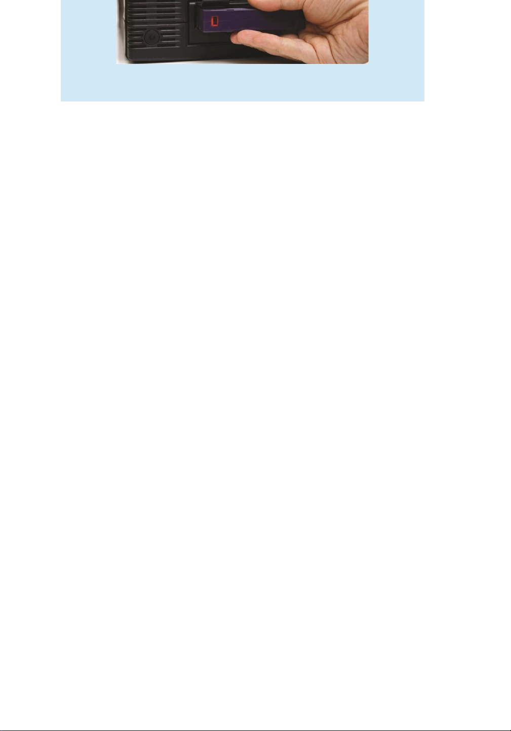
are named according to technology, such as LTO-6 (Figure 11.5) and SDLT. lOMoAR cPSD| 58933639 455 11.1
Overview of Mass-Storage Structure
Figure 11.5 An LTO-6 Tape drive with tape cartridge inserted.
Downloaded by Nguyen Linh (nguyenlinh290820252@gmail.com)
data in memory for temporary safekeeping using standard file operations. In fact, RAM drive
functionality is useful enough that such drives are found in all major operating systems. On
Linux there is /dev/ram, on macOS the diskutil command creates them, Windows has them
via third-party tools, and Solaris and Linux create /tmp at boot time of type “tmpfs”, which is a RAM drive.
RAM drives are useful as high-speed temporary storage space. Although NVM devices are
fast, DRAM is much faster, and I/O operations to RAM drives are the fastest way to create, read,
write, and delete files and their contents. Many programs use (or could benefit from using)
RAM drives for storing temporary files. For example, programs can share data easily by writing
and reading files from a RAM drive. For another example, Linux at boot time creates a
temporary root file system (initrd) that allows other parts of the system to have access to a root
file system and its contents before the parts of the operating system that understand storage devices are loaded. 11.1.4
Secondary Storage Connection Methods
A secondary storage device is attached to a computer by the system bus or an I/O bus. Several
kinds of buses are available, including advanced technology attachment (ATA), serial ATA
(SATA), eSATA, serial attached SCSI (SAS), universal serial bus (USB), and fibr channel (FC).
The most common connection method is SATA. Because NVM devices are much faster than
HDDs, the industry created a special, fast interface for NVM devices called NVM express
(NVMe). NVMe directly connects the device to the system PCI bus, increasing throughput and
decreasing latency compared with other connection methods.
The data transfers on a bus are carried out by special electronic processors called
controllers (or host-bus adapters (HBA)). The host controller is the controller at the
computer end of the bus. A device controller is built into each storage device. To perform a
mass storage I/O operation, the computer places a command into the host controller, typically
using memory-mapped I/O ports, as described in Section 12.2.1. The host controller then sends
the command via messages to the device controller, and the controller operates the drive
hardware to carry out the command. Device controllers usually have a built-in cache. Data
transfer at the drive happens between the cache and the storage media, and data transfer to the
host, at fast electronic speeds, occurs between the cache host DRAM via DMA. 11.1.5 Address Mapping
Storage devices are addressed as large one-dimensional arrays of logical blocks, where the
logical block is the smallest unit of transfer. Each logical block maps to a physical sector or
semiconductor page. The one-dimensional array of logical blocks is mapped onto the sectors
or pages of the device. Sector 0 could be the first sector of the first track on the outermost
cylinder on an HDD, for example. The mapping proceeds in order through that track, then
through the rest of the tracks on that cylinder, and then through the rest of the cylinders, from
outermost to innermost. For NVM the mapping is from a tuple (finite ordered list) of chip,
block, and page to an array of logical blocks. A logical block address (LBA) is easier for
algorithms to use than a sector, cylinder, head tuple or chip, block, page tuple. lOMoAR cPSD| 58933639 456
By using this mapping on an HDD, we can—at least in theory—convert a logical block
number into an old-style disk address that consists of a cylinder number, a track number within
that cylinder, and a sector number within that track. In practice, it is difficult to 11.1
Overview of Mass-Storage Structure
perform this translation, for three reasons. First, most drives have some defective sectors, but
the mapping hides this by substituting spare sectors from elsewhere on the drive. The logical
block address stays sequential, but the physical sector location changes. Second, the number
of sectors per track is not a constant on some drives. Third, disk manufacturers manage LBA to
physical address mapping internally, so in current drives there is little relationship between
LBA and physical sectors. In spite of these physical address vagaries, algorithms that deal with
HDDs tend to assume that logical addresses are relatively related to physical addresses. That is,
ascending logical addresses tend to mean ascending physical address.
Let’s look more closely at the second reason. On media that use constant linear velocity
(CLV), the density of bits per track is uniform. The farther a track is from the center of the disk,
the greater its length, so the more sectors it can lOMoAR cPSD| 58933639 457 11.2 HDD Scheduling
hold. As we move from outer zones to inner zones, the number of sectors per track
decreases. Tracks in the outermost zone typically hold 40 percent more sectors than do
tracks in the innermost zone. The drive increases its rotation speed as the head moves
from the outer to the inner tracks to keep the same rate of data moving under the head.
This method is used in CD-ROM and DVD-ROM drives. Alternatively, the disk rotation
speed can stay constant; in this case, the density of bits decreases from inner tracks to
outer tracks to keep the data rate constant (and performance relatively the same no matter
where data is on the drive). This method is used in hard disks and is known as constant
angular velocity (CAV).
The number of sectors per track has been increasing as disk technology improves,
and the outer zone of a disk usually has several hundred sectors per track. Similarly, the
number of cylinders per disk has been increasing; large disks have tens of thousands of cylinders.
Note that there are more types of storage devices than are reasonable to cover in an
operating systems text. For example, there are “shingled magnetic recording” hard drives
with higher density but worse performance than mainstream HDDs (see
http://www.tomsitpro.com/articles/ shingled-magnetic-recoding-smr-101-basics,2-933.html).
There are also combination devices that include NVM and HDD technology, or volume
managers (see Section 11.5) that can knit together NVM and HDD devices into a storage
unit faster than HDD but lower cost than NVM. These devices have different
characteristics from the more common devices, and might need different caching and
scheduling algorithms to maximize performance. 11.2 HDD Scheduling
One of the responsibilities of the operating system is to use the hardware efficiently. For
HDDs, meeting this responsibility entails minimizing access time and maximizing data transfer bandwidth.
For HDDs and other mechanical storage devices that use platters, access time has two
major components, as mentioned in Section 11.1. The seek time is the time for the device
arm to move the heads to the cylinder containing the desired sector, and the rotational
latency is the additional time for the platter to rotate the desired sector to the head. The
device bandwidth is the total number of bytes transferred, divided by the total time
between the first request for service and the completion of the last transfer. We can
improve both the access time and the bandwidth by managing the order in which storage I/O requests are serviced.
Whenever a process needs I/O to or from the drive, it issues a system call to the
operating system. The request specifies several pieces of information:
• Whether this operation is input or output
• The open file handle indicating the file to operate on lOMoAR cPSD| 58933639 458
• What the memory address for the transfer is
• The amount of data to transfer
If the desired drive and controller are available, the request can be serviced immediately. If
the drive or controller is busy, any new requests for service will be placed in the queue of pending
requests for that drive. For a multiprogramming system with many processes, the device queue
may often have several pending requests.
The existence of a queue of requests to a device that can have its performance optimized by
avoiding head seeks allows device drivers a chance to improve performance via queue ordering.
In the past, HDD interfaces required that the host specify which track and which head to use,
and much effort was spent on disk scheduling algorithms. Drives newer than the turn of the
century not only do not expose these controls to the host, but also map LBA to physical addresses
under drive control. The current goals of disk scheduling include fairness, timeliness, and
optimizations, such as bunching reads or writes that appear in sequence, as drives perform best
with sequential I/O. Therefore some scheduling effort is still useful. Any one of several disk-
scheduling algorithms can be used, and we discuss them next. Note that absolute knowledge of
head location and physical block/cylinder locations is generally not possible on modern drives.
But as a rough approximation, algorithms can assume that increasing LBAs mean increasing
physical addresses, and LBAs close together equate to physical block proximity. 11.2.1 FCFS Scheduling
The simplest form of disk scheduling is, of course, the first-come, first-served (FCFS) algorithm
(or FIFO). This algorithm is intrinsically fair, but it generally does not provide the fastest service.
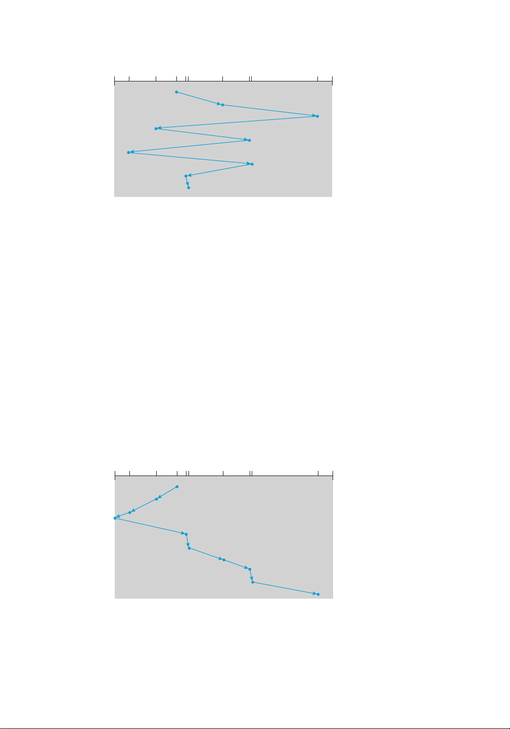
Consider, for example, a disk queue with requests for I/O to blocks on cylinders
98, 183, 37, 122, 14, 124, 65, 67,
in that order. If the disk head is initially at cylinder 53, it will first move from 53 to 98, then to
183, 37, 122, 14, 124, 65, and finally to 67, for a total head movement of 640 cylinders. This
schedule is diagrammed in Figure 11.6.
The wild swing from 122 to 14 and then back to 124 illustrates the problem with this schedule.
If the requests for cylinders 37 and 14 could be serviced together, before or after the requests for
122 and 124, the total head movement could be decreased substantially, and performance could be thereby improved. 11.2.2 SCAN Scheduling
In the SCAN algorithm, the disk arm starts at one end of the disk and moves toward the other
end, servicing requests as it reaches each cylinder, until it gets to the other end of the disk. At the
other end, the direction of head movement is reversed, and servicing continues. The head
continuously scans back and forth across the disk. The SCAN algorithm is sometimes called the
elevator algorithm, since the disk arm behaves just like an elevator in a building, first servicing
all the requests going up and then reversing to service requests the other way.
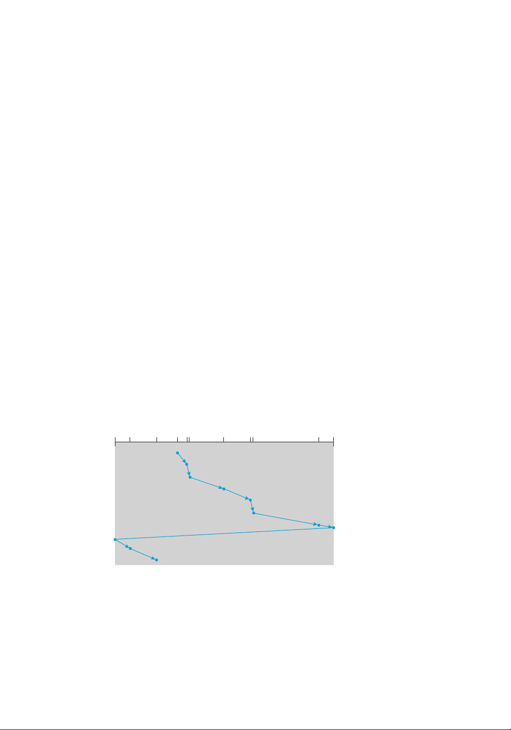
Let’s return to our example to illustrate. Before applying SCAN to schedule the requests on
cylinders 98, 183, 37, 122, 14, 124, 65, and 67, we need to know 11.2 HDD Scheduling
queue = 98, 183, 37, 122, 14, 124, 65, 67 lOMoAR cPSD| 58933639 459 head starts at 53 0 14 37 53 65 67 98 122 124 183199
Figure11.6 FCFSdiskscheduling.
the direction of head movement in addition to the head’s current position. Assuming that the disk
arm is moving toward 0 and that the initial head position is again 53, the head will next service
37 and then 14. At cylinder 0, the arm will reverse and will move toward the other end of the
disk, servicing the requests at 65, 67, 98, 122, 124, and 183 (Figure 11.7). If a request arrives in
the queue just in front of the head, it will be serviced almost immediately; a request arriving just
behind the head will have to wait until the arm moves to the end of the disk, reverses direction, and comes back.
Assuming a uniform distribution of requests for cylinders, consider the density of requests
when the head reaches one end and reverses direction. At this point, relatively few requests are
immediately in front of the head, since these cylinders have recently been serviced. The heaviest
density of requests is at the other end of the disk. These requests have also waited the longest, so
why not go there first? That is the idea of the next algorithm.
queue = 98, 183, 37, 122, 14, 124, 65, 67 head starts at 53 0 14 37 53 65 67 98 122 124 183199
Figure11.7 SCANdiskscheduling. 11.2.3 C-SCAN Scheduling lOMoAR cPSD| 58933639 460
Circular SCAN (C-SCAN) scheduling is a variant of SCAN designed to provide a more uniform
wait time. Like SCAN, C-SCAN moves the head from one end of the disk to the other, servicing
requests along the way. When the head reaches the other end, however, it immediately returns to
the beginning of the disk without servicing any requests on the return trip.
Let’s return to our example to illustrate. Before applying C-SCAN to schedule the requests on
cylinders 98, 183, 37, 122, 14, 124, 65, and 67, we need to know the direction of head movement
in which the requests are scheduled. Assuming that the requests are scheduled when the disk arm
is moving from 0 to 199 and that the initial head position is again 53, the request will be served
as depicted in Figure 11.8. The C-SCAN scheduling algorithm essentially treats the cylinders as a
circular list that wraps around from the final cylinder to the first one. 11.2.4
Selection of a Disk-Scheduling Algorithm
There are many disk-scheduling algorithms not included in this coverage, because they are rarely
used. But how do operating system designers decide which to implement, and deployerschose the
best to use? For any particular list of requests, we can define an optimal order of retrieval, but the
computation needed to find an optimal schedule may not justify the savings over SCAN. With any
scheduling algorithm, however, performance depends heavily on the number and types of
requests. For instance, suppose that the queue usually has just one outstanding request. Then, all
scheduling algorithms behave the same, because they have only one choice of where to move the
disk head: they all behave like FCFS scheduling.
SCAN and C-SCAN perform better for systems that place a heavy load on the disk, because
they are less likely to cause a starvation problem. There can still be starvation though, which
drove Linux to create the deadline scheduler. This scheduler maintains separate read and write
queues, and gives reads priority because processes are more likely to block on read than write. The queues are
queue = 98, 183, 37, 122, 14, 124, 65, 67 head starts at 53 0 14 37 53 65 67 98 122 124 183199
Figure11.8 C-SCANdiskscheduling. 11.3 NVM Scheduling
sorted in LBAorder, essentially implementing C-SCAN. All I/O requests are sent in a batch
in this LBA order. Deadline keeps four queues: two read and two write, one sorted by
LBA and the other by FCFS. It checks after each batch to see if there are requests in the lOMoAR cPSD| 58933639 461
FCFS queues older than a configured age (by default, 500 ms). If so, the LBA queue (read
or write) containing that request is selected for the next batch of I/O.
The deadline I/O scheduler is the default in the Linux RedHat 7 distribution, but
RHEL 7 also includes two others. NOOP is preferredfor CPU-bound systems using fast
storage such as NVM devices, and the Completely Fair Queueing scheduler (CFQ) is
the default for SATA drives. CFQ maintains three queues (with insertion sort to keep them
sorted in LBA order): real time, best effort (the default),and idle.Each has
exclusivepriority overthe others, in that order,with starvation possible. It uses historical
data, anticipating if a process will likely issue more I/O requests soon. If it so determines,
it idles waiting for the new I/O, ignoring other queued requests. This is to minimize seek
time, assuming locality of reference of storage I/O requests, per process. Details of these schedulers can be found in
https://access.redhat.com/site/documentation/en-US /Red Hat Enterprise
Linux/7/html/Performance Tuning Guide/index.html. 11.3 NVM Scheduling
The disk-scheduling algorithms just discussed apply to mechanical platterbased storage
like HDDs. They focus primarily on minimizing the amount of disk head movement.
NVM devices do not contain moving disk heads and commonly use a simple FCFS policy.
For example, the Linux NOOP scheduler uses an FCFS policy but modifies it to merge
adjacent requests. The observed behavior of NVM devices indicates that the time required
to service reads is uniform but that, because of the properties of flash memory, write
service time is not uniform. Some SSD schedulers have exploited this property and merge
only adjacent write requests, servicing all read requests in FCFS order.
As we have seen, I/O can occur sequentially or randomly. Sequential access is
optimal for mechanical devices like HDD and tape because the data to be read or written
is near the read/write head. Random-access I/O, which is measuredin
input/outputoperationspersecond (IOPS), causes HDD disk head movement. Naturally,
random access I/O is much faster on NVM. An HDD can produce hundreds of IOPS, while
an SSD can produce hundreds of thousands of IOPS.
NVM devices offer much less of an advantage for raw sequential throughput, where
HDD head seeks are minimized and reading and writing of data to the media are
emphasized. In those cases, for reads, performance for the two types of devices can range
from equivalent to an order of magnitude advantage for NVM devices. Writing to NVM
is slower than reading, decreasing the advantage. Furthermore, while write performance
for HDDs is consistent throughout the life of the device, write performance for NVM
devices varies depending on how full the device is (recall the need for garbage collection
and over-provisioning) and how “worn” it is. An NVM device near its end of life due to
many erase cycles generally has much worse performance than a new device.
One way to improve the lifespan and performance of NVM devices over time is to
have the file system inform the device when files are deleted, so that the device can erase
the blocks those files were stored on. This approach is discussed further in Section 14.5.6. lOMoAR cPSD| 58933639 462
Let’s look more closely at the impact of garbage collection on performance.
Consider an NVM device under random read and write load. Assume that all blocks have
been written to, but there is free space available. Garbage collection must occur to
reclaim space taken by invalid data. That means that a write might cause a read of one
or more pages, a write of the good data in those pages to overprovisioning space, an
erase of the all-invalid-data block, and the placement of that block into overprovisioning
space. In summary, one write request eventually causes a page write (the data), one or
more page reads (by garbage collection), and one or more page writes (of good data from
the garbage-collected blocks). The creation of I/O requests not by applications but by the
NVM device doing garbage collection and space management is called write
amplificatio and can greatly impact the write performance of the device. In the worst
case, several extra I/Os are triggered with each write request.
11.4 Error Detection and Correction
Error detection and correction are fundamental to many areas of computing, including
memory, networking, and storage. Error detection determines if a problem has occurred
— for example a bit in DRAM spontaneously changed from a 0 to a 1, the contents of a
network packet changed during transmission, or a block of data changed between when
it was written and when it was read. By detecting the issue, the system can halt an
operation before the error is propagated, report the error to the user or administrator, or
warn of a device that might be starting to fail or has already failed.
Memory systems have long detected certain errors by using parity bits. In this
scenario, each byte in a memory system has a parity bit associated with it that records
whether the number of bits in the byte set to 1 is even (parity = 0) or odd (parity = 1). If
one of the bits in the byte is damaged (either a 1 becomes a 0, or a 0 becomes a 1), the
parity of the byte changes and thus does not match the stored parity. Similarly, if the
stored parity bit is damaged, it does not match the computed parity. Thus, all single-bit
errors are detected by the memory system. A double-bit-error might go undetected,
however. Note that parity is easily calculated by performing an XOR (for “eXclusive
OR”) of the bits. Also note that for every byte of memory, we now need an extra bit of memory to store the parity.
Parity is one form of checksums, which use modular arithmetic to compute, store,
and compare values on fixed-length words. Another error-detection method, common in
networking, is a cyclic redundancy check (CRCs), which uses a hash function to detect
multiple-bit errors (see http://www.mathpages.com/home/kmath458/kmath458.htm).
An error-correction code (ECC) not only detects the problem, but also corrects it.
The correction is done by using algorithms and extra amounts of storage. The codes vary
based on how much extra storage they need and how many errors they can correct. For
example, disks drives use per-sector ECC and 11.5
Storage Device Management
flash drives per-page ECC. When the controller writes a sector/page of data during
normal I/O, the ECC is written with a value calculated from all the bytes in the data being
written. When the sector/page is read, the ECC is recalculated and compared with the
stored value. If the stored and calculated numbers are different, this mismatch indicates lOMoAR cPSD| 58933639 463
that the data have become corrupted and that the storage media may be bad (Section
11.5.3). The ECC is error correcting because it contains enough information, if only a
few bits of data have been corrupted, to enable the controller to identify which bits have
changed and calculate what their correct values should be. It then reports a recoverable
soft error. If too many changes occur, and the ECC cannot correct the error, a
noncorrectable hard error is signaled. The controller automatically does the ECC
processing whenever a sector or page is read or written.
Error detection and correction are frequently differentiators between consumer
products and enterprise products. ECC is used in some systems for DRAM error correction
and data path protection, for example.
11.5 Storage Device Management
The operating system is responsible for several other aspects of storage device
management, too. Here, we discuss drive initialization, booting from a drive, and badblock recovery. 11.5.1
Drive Formatting, Partitions, and Volumes
Anew storage device is a blank slate: it is just a platter of a magnetic recording material
or a set of uninitialized semiconductor storage cells. Before a storage device can store
data, it must be divided into sectors that the controller can read and write. NVM pages
must be initialized and the FTLcreated. This process is called low-level formatting, or
physical formatting. Low-level formatting fills the device with a special data structure
for each storage location. The data structure for a sector or page typically consists of a
header, a data area, and a trailer. The header and trailer contain information used by the
controller, such as a sector/page number and an error detection or correction code.
Most drives are low-level-formatted at the factory as a part of the manufacturing
process. This formatting enables the manufacturer to test the device and to initialize the
mapping from logical block numbers to defect-free sectors or pages on the media. It is
usually possible to choose among a few sector sizes, such as 512 bytes and 4KB.
Formatting a disk with a larger sector size means that fewer sectors can fit on each track,
but it also means that fewer headers and trailers are written on each track and more space
is available for user data. Some operating systems can handle only one specific sector size.
Before it can use a drive to hold files, the operating system still needs to record its
own data structures on the device. It does so in three steps.
The first step is to partition the device into one or more groups of blocks or pages.
The operating system can treat each partition as though it were a separate device. For
instance, one partition can hold a file system containing a copy of the operating system’s
executable code, another the swap space, and another a file system containing the user
files. Some operating systems and file systems perform the partitioning automatically
when an entire device is to be managed by the file system. The partition information is
written in a fixed format at a fixed location on the storage device. In Linux, the fdisk
command is used to manage partitions on storage devices. The device, when recognized
by the operating system, has its partition information read, and the operating system then lOMoAR cPSD| 58933639 464
creates device entries for the partitions (in /dev in Linux). From there, a configuration
file, such as /etc/fstab, tells the operating system to mount each partition containing a
file system at a specified location and to use mount options such as read-only. Mounting
a file system is making the file system available for use by the system and its users.
The second step is volume creation and management. Sometimes, this step is implicit, as
when a file system is placed directly within a partition. That volume is then ready to be mounted
and used. At other times, volume creation and management is explicit—for example when
multiple partitions or devices will be used together as a RAID set (see Section 11.8) with one or
more file systems spread across the devices. The Linux volume manager lvm2 can provide these
features, as can commercial third-party tools for Linux and other operating systems. ZFS provides
both volume management and a file system integrated into one set of commands and features.
(Note that “volume” can also mean any mountable file system, even a file containing a file system such as a CD image.)
The third step is logical formatting, or creation of a file system. In this step, the operating
system stores the initial file-system data structures onto the device. These data structures may
include maps of free and allocated space and an initial empty directory.
The partition information also indicates if a partition contains a bootable file system
(containing the operating system). The partition labeled for boot is used to establish the root of
the file system. Once it is mounted, device links for all other devices and their partitions can be
created. Generally, a computer’s “file system” consists of all mounted volumes. On Windows,
these are separately named via a letter (C:, D:, E:). On other systems, such as Linux, at boot time
the boot file system is mounted, and other file systems can be mounted within that tree structure
(as discussed in Section 13.3). On Windows, the file system interface makes it clear when a given
device is being used, while in Linux a single file access might traverse many devices before the
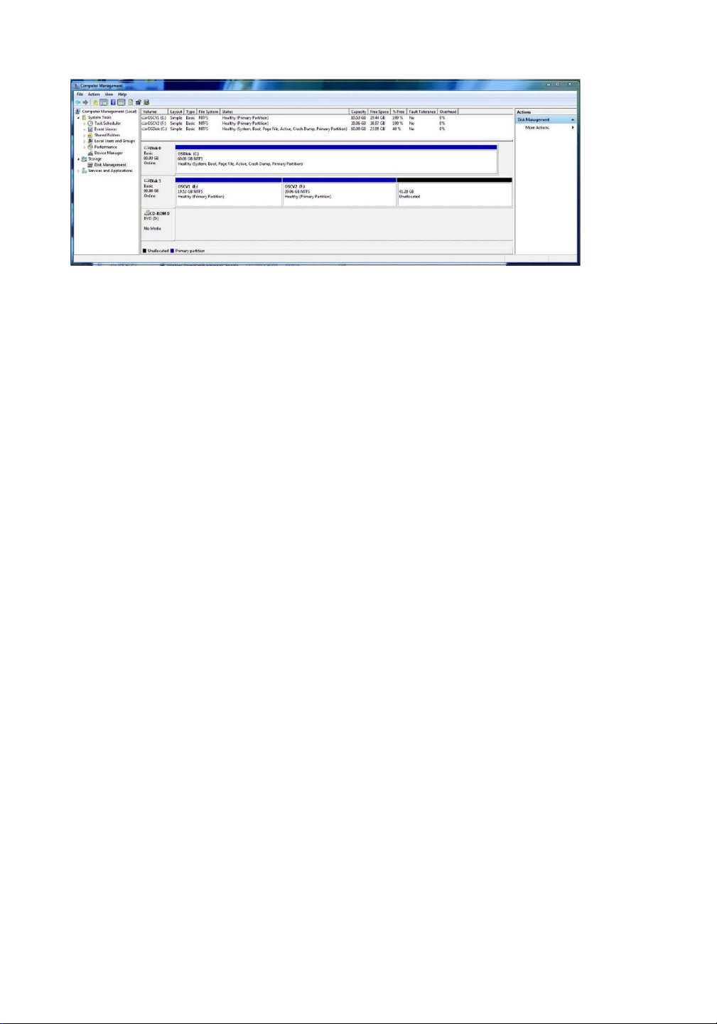
requested file in the requested file system (within a volume) is accessed. Figure 11.9 shows the
Windows 7 Disk Management tool displaying three volumes (C:, E:, and F:). Note that E: and
F: are each in a partition of the “Disk 1” device and that there is unallocated space on that device
for more partitions (possibly containing file systems).
To increase efficiency, most file systems group blocks together into larger chunks, frequently
called clusters. Device I/O is done via blocks, but file system I/O is done via clusters, effectively
assuring that I/O has more sequential-access and fewer random-access characteristics. File
systems try to group file contents near its metadata as well, reducing HDD head seeks when
operating on a file, for example.
Some operating systems give special programs the ability to use a partition as a large
sequential array of logical blocks, without any file-system data structures. This array is sometimes
called the raw disk, and I/O to this array is termed raw I/O. It can be used for swap space (see
Section 11.6.2), for example, and some database systems prefer raw I/O because it enables them to control 11.5
Storage Device Management lOMoAR cPSD| 58933639 465 Figure 11.9
Windows 7 Disk Management tool showing devices, partitions, volumes, and file systems.
the exact location where each database record is stored. Raw I/O bypasses all the file-system
services, such as the buffer cache, file locking, prefetching, space allocation, file names, and
directories. We can make certain applications more efficient by allowing them to implement their
own special-purpose storage services on a raw partition, but most applications use a provided file
system rather than managing data themselves. Note that Linux generally does not support raw I/O
but can achieve similar access by using the DIRECT flag to the open() system call. 11.5.2 Boot Block
For a computer to start running—for instance, when it is powered up or rebooted—it must have
an initial program to run. This initial bootstrap loader tends to be simple. For most computers,
the bootstrap is stored in NVM flash memory firmware on the system motherboard and mapped
to a known memory location. It can be updated by product manufacturers as needed, but also can
be written to by viruses, infecting the system. It initializes all aspects of the system, from CPU
registers to device controllers and the contents of main memory.
This tiny bootstrap loader program is also smart enough to bring in a full bootstrap program
from secondary storage. The full bootstrap program is stored in the “boot blocks” at a fixed location on the device. The default Linux bootstrap loader is grub2
(https://www.gnu.org/software/grub/manual/ grub.html/). A device that has a boot partition is called
a boot disk or system disk.
The code in the bootstrap NVM instructs the storage controller to read the boot blocks into
memory (no device drivers are loaded at this point) and then starts executing that code. The full
bootstrap program is more sophisticated than the bootstrap loader: it is able to load the entire
operating system from a non-fixed location on the device and to start the operating system running.
Let’s consider as an example the boot process in Windows. First, note that Windows allows
a drive to be divided into partitions, and one partition— identified as the boot partition—
contains the operating system and device drivers. The Windows system places its boot code in
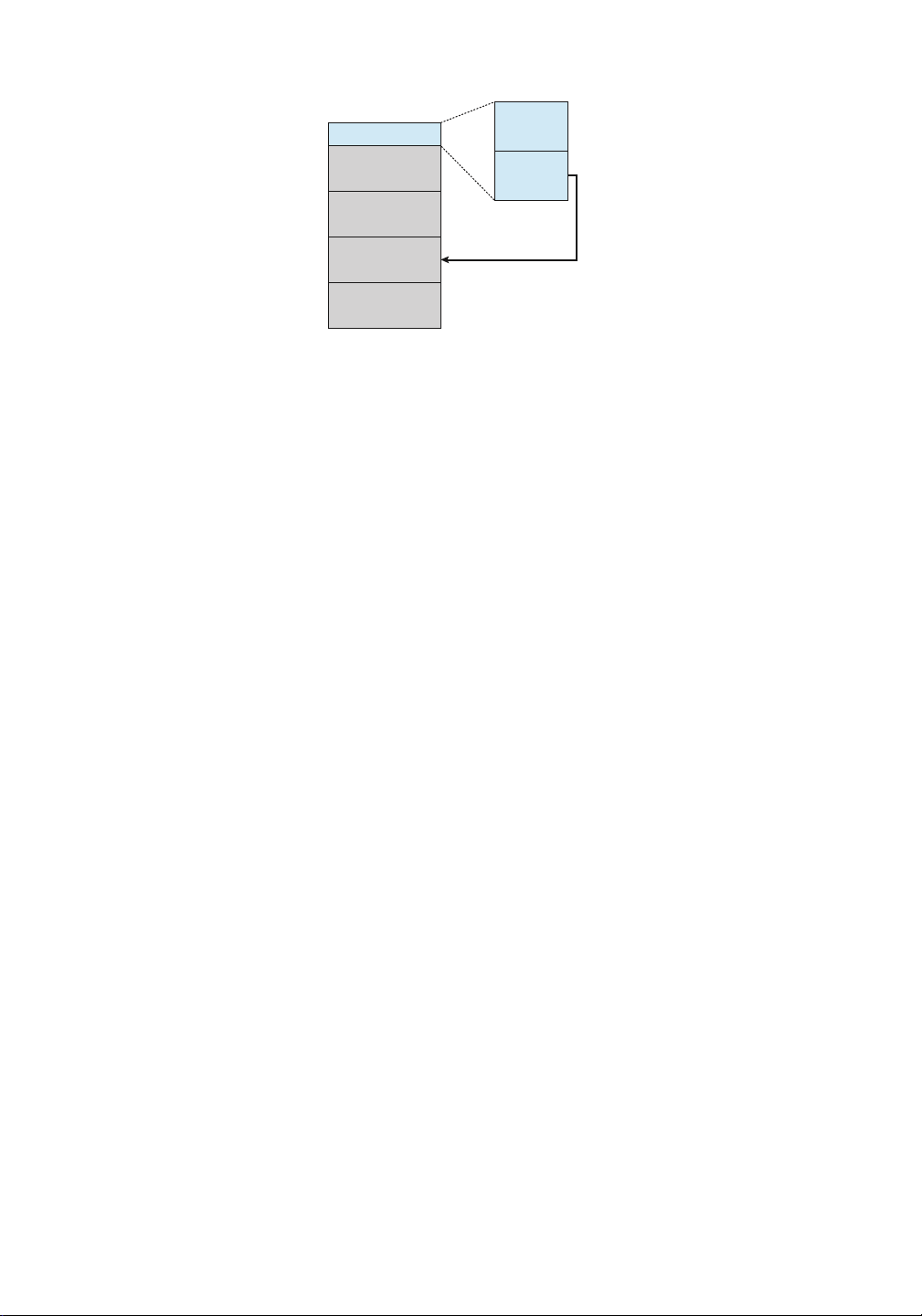
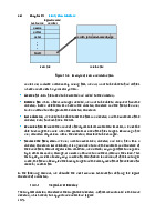
the first logical block on the hard disk or first page of the NVM device, which it terms the master boot lOMoAR cPSD| 58933639 466 boot MBR code partition 1 partition table partition 2 boot partition partition 3 partition 4
Figure 11.10 Booting from a storage device in Windows.
record, or MBR. Booting begins by running code that is resident in the system’s firmware. This
code directs the system to read the boot code from the MBR, understanding just enough about the
storage controller and storage device to load a sector from it. In addition to containing boot code,
the MBR contains a table listing the partitions for the drive and a flag indicating which partition
the system is to be booted from, as illustrated in Figure 11.10. Once the system identifies the boot
partition, it reads the first sector/page from that partition (called the boot sector), which directs
it to the kernel. It then continues with the remainder of the boot process, which includes loading
the various subsystems and system services. 11.5.3 Bad Blocks
Because disks have moving parts and small tolerances (recall that the disk head flies just above
the disk surface), they are prone to failure. Sometimes the failure is complete; in this case, the
disk needs to be replaced and its contents restored from backup media to the new disk. More
frequently, one or more sectors become defective. Most disks even come from the factory with
bad blocks. Depending on the disk and controller in use, these blocks are handled in a variety of ways.
On older disks, such as some disks with IDE controllers, bad blocks are handled manually.
One strategy is to scan the disk to find bad blocks while the disk is being formatted. Any bad
blocks that are discovered are flagged as unusable so that the file system does not allocate them.
If blocks go bad during normal operation, a special program (such as the Linux badblocks
command) must be run manually to search for the bad blocks and to lock them away. Data that
resided on the bad blocks usually are lost.
More sophisticated disks are smarter about bad-block recovery. The controller maintains a
list of bad blocks on the disk. The list is initialized during the low-level formatting at the factory
and is updated over the life of the disk. Low-level formatting also sets aside spare sectors not
visible to the operating system. The controller can be told to replace each bad sector logically
with one of the spare sectors. This scheme is known as sector sparing or forwarding.
A typical bad-sector transaction might be as follows: • The
operating system tries to read logical block 87. 11.6 Swap-Space Management lOMoAR cPSD| 58933639 467
• The controller calculates the ECC and finds that the sector is bad. It reports this
finding to the operating system as an I/O error.
• The device controller replaces the bad sector with a spare.
• After that, whenever the system requests logical block 87, the request is translated
into the replacement sector’s address by the controller.
Note that such a redirection by the controller could invalidate any optimization by
the operating system’s disk-scheduling algorithm! For this reason, most disks are
formatted to provide a few spare sectors in each cylinder and a spare cylinder as well.
When a bad block is remapped, the controller uses a spare sector from the same cylinder, if possible.
As an alternative to sector sparing, some controllers can be instructed to replace a
bad block by sector slipping. Here is an example: Suppose that logical block 17 becomes
defective and the first available spare follows sector 202. Sector slipping then remaps all
the sectors from 17 to 202, moving them all down one spot. That is, sector 202 is copied
into the spare, then sector 201 into 202, then 200 into 201, and so on, until sector 18 is
copied into sector 19. Slipping the sectors in this way frees up the space of sector 18 so
that sector 17 can be mapped to it.
Recoverable soft errors may trigger a device activity in which a copy of the block
data is made and the block is spared or slipped. An unrecoverable hard error, however,
results in lost data. Whatever file was using that block must be repaired (for instance, by
restoration from a backup tape), and that requires manual intervention.
NVM devices also have bits, bytes, and even pages that either are nonfunctional at
manufacturing time or go bad over time. Management of those faulty areas is simpler
than for HDDs because there is no seek time performance loss to be avoided. Either
multiple pages can be set aside and used as replacement locations, or space from the
over-provisioning area can be used (decreasing the usable capacity of the
overprovisioning area). Either way, the controller maintains a table of bad pages and
never sets those pages as available to write to, so they are never accessed. 11.6 Swap-Space Management
Swapping was first presented in Section 9.5, where we discussed moving entire
processes between secondary storage and main memory. Swapping in that setting occurs
when the amount of physical memory reaches a critically low point and
processesaremovedfrom memory to swap space to freeavailable memory. In practice,
very few modern operating systems implement swapping in this fashion. Rather, systems
now combine swapping with virtual memory techniques (Chapter 10) and swap pages,
not necessarily entire processes. In fact, some systems now use the terms “swapping”
and “paging” interchangeably, reflecting the merging of these two concepts.
Swap-space management is another low-level task of the operating system. Virtual
memory uses secondary storage space as an extension of main memory. Since drive
access is much slower than memory access, using swap space significantly decreases
system performance. The main goal for the design and implementation of swap space is lOMoAR cPSD| 58933639 468
to provide the best throughput for the virtual memory system. In this section, we discuss
how swap space is used, where swap space is located on storage devices, and how swap space is managed. 11.6.1 Swap-Space Use
Swap space is used in various ways by different operating systems, depending on the
memorymanagement algorithms in use. For instance, systems that implement swapping may use
swap space to hold an entire process image, including the code and data segments. Paging systems
may simply store pages that have been pushed out of main memory. The amount of swap space
needed on a system can therefore vary from a few megabytes of disk space to gigabytes,
depending on the amount of physical memory, the amount of virtual memory it is backing, and
the way in which the virtual memory is used.
Note that it may be safer to overestimate than to underestimate the amount of swap space
required, because if a system runs out of swap space it may be forced to abort processes or may
crash entirely. Overestimation wastes secondary storage space that could otherwise be used for
files, but it does no other harm. Some systems recommend the amount to be set aside for swap
space. Solaris, for example, suggests setting swap space equal to the amount by which virtual
memory exceeds pageable physical memory. In the past, Linux has suggested setting swap space
to double the amount of physical memory. Today, the paging algorithms have changed, and most
Linux systems use considerably less swap space.
Some operating systems—including Linux—allow the use of multiple swap spaces, including
both files and dedicated swap partitions. These swap spaces are usually placed on separate storage
devices so that the load placed on the I/O system by paging and swapping can be spread over the system’s I/O bandwidth. 11.6.2 Swap-Space Location
Aswap space can reside in one of two places: it can be carved out of the normal file system, or it
can be in a separate partition. If the swap space is simply a large file within the file system, normal
file-system routines can be used to create it, name it, and allocate its space.
Alternatively, swap space can be created in a separate raw partition. No file system or
directory structure is placed in this space. Rather, a separate swap-space storage manager is used
to allocate and deallocate the blocks from the raw partition. This manager uses algorithms
optimized for speed rather than for storage efficiency, because swap space is accessed much more
frequently than file systems, when it is used (recall that swap space is used for swapping and
paging). Internal fragmentation may increase, but this tradeoff is acceptable because the life of
data in the swap space generally is much shorter than that of files in the file system. Since swap
space is reinitialized at boot time, any fragmentation is short-lived. The raw-partition approach
creates a fixed amount of swap space during disk partitioning. Adding more swap space requires
either repartitioning the device (which involves moving
11.7 Storage Attachment
the other file-system partitions or destroying them and restoring them from backup) or
adding another swap space elsewhere.
Some operating systems are flexible and can swap both in raw partitions and in file-
system space. Linux is an example: the policy and implementation are separate, allowing
Tài liệu liên quan:
-
Chapter 13: File-System Interface in Abraham-Silberschatz's OS Concepts | Môn Cơ sở hệ điều hành - Đại học Xây Dựng Hà Nội
146 73 -
Distributed Systems Overview: Concepts and Protocols in Networking | Môn Cơ sở hệ điều hành - Đại học Xây Dựng Hà Nội
123 62 -
Virtualization: Understanding Its Role in Modern Computing Environments | Môn Cơ sở hệ điều hành - Đại học Xây Dựng Hà Nội
116 58 -
Làm Quen Với Hệ Điều Hành Linux | Môn Cơ sở hệ điều hành - Đại học Xây Dựng Hà Nội
107 54