Chapter 2: understanding random variables and their properties môn Xác suất thống kê| Trường Đại học Ngoại Thương
A variable is said to be a random variable if in the result of a trialit will take one and only one of its possible values randomly with some corresponding probabilities. Tài liệu giúp bạn tham khảo, ôn tập và đạt kết quả cao. Mời đọc đón xem!
Môn: Xác suất thống kê (FTU) 355 tài liệu
Trường: Trường Đại học Ngoại Thương 1.1 K tài liệu
Tác giả:


Preview text:
Chapter 2. Random variables
2.1 The concept of random variables 2.1.1 Definition
A variable is said to be a random variable if in the result of a trial it wil take one and
only one of its possible values randomly with some corresponding probabilities.
We usually denote random variables by the letters X, Y, Z …
2.2.2 Classification of random variables 1) Discrete random variables
Definition. A random variable is said to be a discrete random variable if the set of the
possible values of this random variable is either a finite set or an infinite but countable set.
Example 1. Rol a dice. Let X be the number of dots obtained. Then, X is a discrete
random variable because the set of the possible values of X is a finite set 1, 2, 3, 4, 5, . 6
Example 2. Let Y be the number of people shopping at a supermarket in a day. Then, Y
is a discrete random variable because the set of the possible values of Y is an infinite but countable set 0, 1 , 2 , 3 , .
2) Continuous random variables
Definition. A random variable is said to be a continuous random variable if the set of the
possible values of this random variable fil s a/some interval(s) on the number line, or
even fil s the entire number line.
Example 1. Shoot a bul et at a target. Let X be the distance from the point of impact of
the bul et to the center of the target. X is a continuous random variable because we cannot Lecturer: Nguyen Duong Nguyen
Mathematics Department, Faculty of Basic Science, FTU Page 1
list al the possible values of X. We can only say that the possible values of X are in some interval a, b .
Example 2. Let X be the weight of a type of chicken eggs. X is a continuous random variable.
2.2 The law of the probability distribution of a random variable
2.2.1 Definition. The law of the probability distribution of a random variable is the
determination of the relationship between the possible values of this random variable and
the corresponding probabilities.
2.2.2 Probability distribution table
To describe the law of the probability distribution of a discrete random variable,
we use a probability distribution table.
Suppose a discrete random variable X takes the values x1, x2, …, xn, … (x x ... x
...) with the corresponding probabilities P(X = xi) = pi, for al i = 1, 2, 1 2 n
… The probability distribution table of the discrete random variable X is defined as: X x1 x 2 … x n … P(X = xi) p1 p2 … pn … 0 p 1, for all i = 1, 2, ... where i p1i i
Example. A box contains 10 products including 4 defective products. Randomly draw 2
products from the box to check the quality. Let X be the number of defective products
obtained. Find the probability distribution of X.
Solution. X can take values of 0, 1, 2. We have Lecturer: Nguyen Duong Nguyen
Mathematics Department, Faculty of Basic Science, FTU Page 2 2 C1 P(X = 0) = 6 2 C3 10 11 C .C 8 P(X = 1) = 46 2 C 15 10 2 C2 P(X = 2) = 4 2 C 15 10
The probability distribution table of X is X 0 1 2 P(X = xi) 1/3 8/15 2/15
2.2.3 The distribution function
1) Definition. Let X be any random variable. The function: ( F ) x ( P X < x), x
is cal ed the distribution function (cdf) of X.
Note. If X is a discrete random variable and P(X = xi) = pi, for x R, we have F(x) = p . i i:x x i
So, if X is a discrete random variable that takes the values x , x ,..., x 1 2 n (x x
... x ) with P(X = xi) = pi, for all i = 1, 2, … , we have 1 2 n Lecturer: Nguyen Duong Nguyen
Mathematics Department, Faculty of Basic Science, FTU Page 3 0, if x 1 x p , if x 1 12 pp , if x 12 23 F (x ) ... p p ... , p x x 1 2 1 kk if xk-1 ... 1, if x > xn
Example. Refer to Example in Section 2.2.2. Find the distribution function of X.
Solution. According to Example in Section 2.2.2, we found that the probability distribution table of X is X 0 1 2 P(X = xi) 1/3 8/15 2/15
So, the distribution function of X is: 0,if x 0 1,if 0 x 1 3 F(x) = 18 13 ,if 1 < x 2 3 15 15 18 2 + =1,if x > 2 3 15 15 2) Properties
Let F(x) be the cdf of a random variable X. F(x) has the fol owing properties:
Property 1. 0 F(x) 1, for al x R.
Property 2. F(x) is nondecreasing, which means if x2 > x1, F(x 2) F (x1).
Corol ary 1. P(a X < b) = F(b) – F(a).
Corol ary 2. The probability that the continuous random variable X takes a defined value is equal to zero: Lecturer: Nguyen Duong Nguyen
Mathematics Department, Faculty of Basic Science, FTU Page 4 P(X = x0) = 0.
Corol ary 3. If X is a continuous random variable, we have:
P(a X b) = P(a X < b) = P( a < X b) = P(a < X < b) Property 3. F ( ) lim F (x) , 0 F ( ) lim F ( ) x 1 . xx
Property 4. If X is a continuous random variable F, x is continuous for al xR .
Example. The queuing time for buying goods of customers (unit: minutes) is a
continuous random variable X with a distribution function as fol ows: 0, if x 0 3 F(x) mx 2 1 -3x +2x, if 0 < x 1 1, if x > a) Find m.
b) Find the probability that out of 3 people queuing to buy goods, there are 2 people that
have to wait for more than 0.6 minutes. Solution
a) Since the function F(x) is continuous at x = 1, we have 32 lim F(x)+2 l xim ) =( m m x - 1 3 = x F( ) 1 x 1 x 1 li m F(x) lim1 1 F(1) m 1 x 1 x 1 This leads to m2 . Thus, 0, if x 0 3 F(x) 2x 2 1 -3x +2x,if 0 < x 1 1, if x > Lecturer: Nguyen Duong Nguyen
Mathematics Department, Faculty of Basic Science, FTU Page 5 b) We have P( X > 0.6) = P(0.6 X ) = F( ) – F(0.6) = 1- 32 (2(0.6) 3(0.6) 2(0.6)) = 0.448
Let A be the event "The queuing time for buying goods of customers".
3 people queuing to buy goods are three independent trials. The probability of the
event A occurring in each above trial is equal to 0.448. So, the above 3 trials are 3
Bernoul i trials. The requirement of the problem is to find the probability that in 3
Bernoul i trials, the event A occurs twice. Therefore, according to Bernoul i's formula, the
probability that out of 3 people queuing to buy goods, there are 2 people that have to wait for more than 0.6 minutes is 22 P (2) C (0.448) (0.552) 0.3324 33
2.2.4 The probability density function
To describe the law of the probability distribution of a continuous random variable, we
use a probability density function.
1) Definition: Let F(x) be the distribution function of X. Then, the function f x F x
is cal ed the probability density function (pdf) of X.
Example 1. Let X be a random variable X that has the distribution function Fx 11 2 arctanx
. Find the probability density function of X.
Solution. The probability density function of X is 1 f(x) = F'(x) = . 2 (1 x ) Lecturer: Nguyen Duong Nguyen
Mathematics Department, Faculty of Basic Science, FTU Page 6
Example 2. Let X be a continuous random variable X that has the distribution function as fol ows: 0, if x 0 1 F(x) (1 c osx), if 0 < x 2 1, if x > .
Find the probability density function of X. Solution. +) x < 0: f x F x 0 . +) 0 < x < : 1s f x F x inx . 2 +) x > : f x F x 0 . +) x = 0: F(x) F(0) 0 0 F0 x 0 limx lim 0 x 0 x 0 1(1 c 0 F(x) F(0) osx) osx i 1 nx 1 c 1 s 2 F1 0 lim lim lim lim 0 x 0 x 0 x 0 x x 2 0 x x 0 2 So, f 0 F 0 0 . +) x = : 1(1 c F(x) F( ) osx)-1 os 1 x inx 1 c 1 s 2 F(2 ) lim lim lim lim 0 x x x x x x 2 1 x- Lecturer: Nguyen Duong Nguyen
Mathematics Department, Faculty of Basic Science, FTU Page 7 F(x) F( ) 1 1 0 F(x )x lim lim lim 0 . x x x x 0 Thus, f ( ) F( ) 0 .
Then, the probability density function of X is 0, if x 0 1 f (x) sinx, if 0 2 0, if x >
2) Properties: Let X be a continuous random variable that has the probability density
function f(x) and the distribution function F(x).
Property 1. f(x) 0, for al x (; ) b Property 2. P a x b f (x)dx a b Especial y: P x b f (x)dx; P x a f (x)dx a
Note. Let X be a continuous random variable. We have b
P(a X b) P(a X b) P(a X b) P(a X b) f(x)dx a x Property 3. F(x) = f (t)dt Property 4. f (x)dx 1 Lecturer: Nguyen Duong Nguyen
Mathematics Department, Faculty of Basic Science, FTU Page 8
Example. Let X be a continuous random variable that has the fol owing probability density function: msin2x, if x 0, f(x) = 2 0, if x 0, 2 a) Find m.
b) Find the distribution function of X. 2
c) Compute the probability that X lies between and . 4 3 Solution. a) We have 0 2 2 mc m( 1 1) f (x)dx = 0dx + 2 msin2xdx + 0dx = msin2xdx = - os2x = - 2 = m = 2 0 0 0 2 1 Thus, m = 1.
b) To determine the distribution function, we use the fol owing formula x F(x) = f (t)dt x +) x 0: F(x) = 0dt = 0. +) 0x 2 : Lecturer: Nguyen Duong Nguyen
Mathematics Department, Faculty of Basic Science, FTU Page 9 x 0 x 1c 1(c F(x) = f (t)dt 0dt sin 2tdt = x 2os2t = 2os2x-1) = sin2x. 0 0 +) x > : 2 x 0x 2 1c F(x) = f (t)dt = 0dt sin 2tdt 0dt = 2 2os2t = 1. 0 0 2
So, the distribution function of X is: 0, if x 0 x Fx, 2 sin if 0 1, if x > 2 2 322 2 1 1 c) P 40 X f (x)dx sin 2xdx c 1 0 .5 32 os2x . 2 4 44
2.3 Characteristic parameters of a random variable 2.3. 1 The expected value
1) Definition. The expected value of a random variable X, denoted by E(X), is defined as fol ows:
x p ,if X be a discrete random variable with range {x , x , ..., x , ...} and the corresponding i 1 2 n i E(X) probabilities P(X=xii)=p
xf (x)dx,if X be a continuous ramdom variable and has the probability den)sity f u nction f(x Lecturer: Nguyen Duong Nguyen
Mathematics Department, Faculty of Basic Science, FTU Page 10
The meaningful: The expected value of the random variable X is approximately equal to
the arithmetical mean of the observed values of the random variable X.
Example 1. Find the expected value of a random variable X that has the fol owing
probability distribution table: X -1 0 1 2 P 0.2 p 0.3 0.4
Solution. Since p(X x ) 1, p = 0.1 i i We have
E(X) = -1(0.2) + 0(0.1) + 1(0.3) + 2(0.4) = 0.9.
Example 2. Queuing time for customers to buy goods (unit: minutes) is a continuous
random variable X that has a probability density function as fol ows: 4x 3 f (x) 81 , if x [0;3] 0, if x [0;3]
Find the average queuing time of customers.
Solution. Average customer queuing time is: 03 4 3 4x dx E(X) = xf (x)dx = 4 x.0dx x dx x.0dx = 4 81 81 = 2.4 minutes. 03 0 2) Properties
Property 1. If C is a constant, E(C) = C.
Property 2. If C is a constant and X is a random variable, E(CX) = C.E(X).
Property 3. If X and Y are any two random variables, E(X + Y) = E(X) + E(Y). Lecturer: Nguyen Duong Nguyen
Mathematics Department, Faculty of Basic Science, FTU Page 11
Corrol ary 1. If X and Y are any two random variables, E(X - Y) = E(X) - E(Y).
Definition. Two random variables X and Y are cal ed independent if the probability
distribution of one variable is not affected by the values taken by another.
For example: If X and Y are two discrete random variables, X and Y are independent if and only if P(X x / Y y ) P(X x ) i j i P(Y y / X x ) P(Y y ) j i j
Property 4. Let X and Y be independent random variables. Then E(XY) = E(X).E(Y). Property 5. Let g : be any function. Then g(x )p ,if i i
X is a discrete random variable with range 1 {x 2, x n , ..., x , ...} and the i
corresponding probabilities P(X=x )=p ii E[g(X)] =
g(x)f (x)dx, if X is a continuous ramdom variable and has the probability density function f(x) 2.3.2 The variance
1) Definiton. The variance of a random variable X is a nonnegative number, denoted by V(X), is defined as fol ows:
V(X) = E(X – EX)2 = E(X2) – [E(X)]2 So, Lecturer: Nguyen Duong Nguyen
Mathematics Department, Faculty of Basic Science, FTU Page 12 22 x p [E(X)] ,if is
X a discrete random variable with range {x , x , ..., x , ...} and the i 1 2 n i
corresponding probabilities P(X i =xi)=p V X 22 x f (x)dx [E(X)] , if
X is a continuous ramdom variable and h proba as the bility density f(x) function
The meaningful: The variance reflects the dispersion of the values of the random variable
around its mean, which is the mathematical expectation. In engineering, the variance
characterizes the degree of dispersion of the work pieces or the error of the equipment. In
management and business, it characterizes the degree of risk of decisions.
Example 1. Let X be a random variable that has a probability distribution density function as fol ows: 1s f(x) = 2 inx, if x [0; ] 0, if x [0; ] Find V(X). Solution. We have 1 E(X) = xf (x)dx x sinxdx 22 0 E(X 11 2) = 2 2 2 2 x f (x)dx x sinxdx inxd x x s 2 2 2 2 00 Thus, 2 2 2 V(X) = E(X2) – [E(X)]2 = 2 2 0.4649 . 2 4 4 Lecturer: Nguyen Duong Nguyen
Mathematics Department, Faculty of Basic Science, FTU Page 13
Ví dụ 2. Cho XA và XB lần lượt là lợi nhuận thu được khi đầu tư 100 triệu đồng vào dự án
A và B có các bảng phân phối xác suất như sau:
Example 2. Let XA and XB be the profit obtained from investing 100 mil ion VND in
projects A and B, respectively, with the fol owing probability distribution tables: XA (Unit: mil ion dong) -3 -1 0 1 2 3 P 0.1 0.1 0.2 0.3 0.2 0.1 XB (Unit: mil ion dong) -2 -1 0 1 3 P 0.1 0.2 0.2 0.2 0.3
Which project should invest in to give:
a) The expected profit is higher. b) The level of risk is less. Solution. a) We have
E(XA) = -3(0.1) + (-1)(0.1) + 0(0.2) + 1(0.3) + 2(0.2) + 3(0.1) = 0.6
E(XB) = -2(0.1) + (-1)(0.2) + 0(0.2) + 1(0.2) + 3(0.3) = 0.7 E(XB) > E(XA).
Thus, investing in project B wil bring higher profit than investing in project A. b) We have E( 2
X ) = (-3)2(0.1) + (-1)2(0.1) + 02(0.2) + 12(0.3) + 22(0.2) + 32(0.1) = 3 A Lecturer: Nguyen Duong Nguyen
Mathematics Department, Faculty of Basic Science, FTU Page 14 V(XA) = E( 2
X ) - [E(XA)]2 = 3 – (0.6)2 = 2.64 A E( 2
X ) = (-2)2(0.1) + (-1)2(0.2) + 02(0.2) + 12(0.2) + 32(0.3) = 3.5 B V(XB) = E( 2
X ) - [E(XB)]2 = 3.5 – 0.72 = 3.01 B V(XA) < V(XB).
So, investing in project A is less risky than project B. 2) Properties
Property 1. If C is a constant, V(C) = 0.
Property 2. If C is a constant and X is a random variable, V(CX) = C2V(X).
Property 3. If X and Y are two independent random variables, V(X Y) V(X) V(Y) .
Corol ary 1. If X and Y are two independent random variables, V(X - Y) = V(X) + V(Y).
Corol ary 2. If C is a constant and X is a random variable, V(C + X) = V(X). 2.3.3 The standard deviation
Since we have squared the values, the variance is not on the same scale as X. For
example, if X is weights in grams, the unit of measure of Var(X) is square grams which
does not have a clear meaning. For this reason, we often use the fol owing definition.
Definition. Let X be a random variable. The standard deviation of X, written, is X defined as Lecturer: Nguyen Duong Nguyen
Mathematics Department, Faculty of Basic Science, FTU Page 15 XV(X) . 2.3.4 Mode
Definition. The mode of a random variable X, denoted by Mod(X), is defined as:
If X is a discrete random variable, Mod(X) is the value of X which the
corresponding probability is greatest.
If X is a continuous random variable with a probability density function of f(x),
Mod(X) is the value of x0 which f(x0) is maximal. 2.3.5 Median
Definition. The median of a random variable X, denoted by Med(X), is defined as: 1 P(X MedX) 2 1 P(X MedX) 2
It is easy to see that if X is a continuous random variable, Med(X) is a number satisfying MedX
F(MedX) = 0.5 (or f (x)dx 0.5),
where F(x) and f(x) are the distribution function and the probability density function of X, respectively.
Example 1. Let X be a random variable that has a probability distribution table as X -1 0 1 2 P 0.25 0.15 0.3 0.3 a) Find Mod(X). b) Find Med(X). Lecturer: Nguyen Duong Nguyen
Mathematics Department, Faculty of Basic Science, FTU Page 16 Solution. a) Mod(X) = 1 and Mod(X) = 2. b) We have
P(X 1) 0.4 0.5 ; P(X 1) 0.7 0.5 So, Med(X) = 1.
Example 2. Let X be a random variable that has the fol owing probability density function as 0, if x < 0 2 f (x) x x if x 0 4 e, 2 a) Find Mod(X) b) Find Med(X). Solution. a) We have +) If x 0, f(x) = 0 2 2x 1x +) If x > 0, '4 f (x) e 0 x = 2 . 24 2 2x x 3 x 2 "4 f (x) e " 1/ 2 fe( 2) 0 4 2 2 2 2 1/ 2 f ( e 2) 2
So, f(x) reaches its maximum at x = 2 ModX = 2 . Lecturer: Nguyen Duong Nguyen
Mathematics Department, Faculty of Basic Science, FTU Page 17 x0
b) Suppose MedX = x0. We have F(x0) = 0.5 f (x)dx 0.5 x00 x If x0 ≤ 0, f (x)dx
0dt 0 = 0. So, the values x0 ≤ 0 are not Med(X). x xx 22 0 2 0x xx If x 00 0 x 0 > 0, 4 4 4 f (x)dx 0.dx e dt e 1 e 2 00 2 x 0 4 1 e 0,5 x0 = 2 ln 2 So, MedX = 2 ln 2. Lecturer: Nguyen Duong Nguyen
Mathematics Department, Faculty of Basic Science, FTU Page 18
Tài liệu liên quan:
-
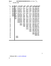
Bảng giá trị phân phối thống kê poisson và student môn Xác suất thống kê| Trường Đại học Ngoại Thương
27 14 -
Bảng giá trị quyết định thống kê wilcoxon rank-sum test môn Xác suất thống kê| Trường Đại học Ngoại Thương
29 15 -
Bài 1 Định nghĩa cổ điển về xác suất môn Xác suất thống kê| Trường Đại học Ngoại Thương
26 13 -
Exercises for probability & statistics môn Xác suất thống kê| Trường Đại học Ngoại Thương
26 13 -
Đề thi cuối kỳ lý thuyết môn Xác suất thống kê| Trường Đại học Ngoại Thương
27 14