Chapter 3 - Giải đáp bài tập và phân tích đồ thị thống kê môn Xác suất thống kê| Trường Đại học Ngoại Thương

Chapter 3 3.1 9 or 10 3.2 10 or 11 3.3 a 7 to 9 188 37 9 . 18 b Interval width 8
(rounded to 20); upper limits: 40, 60, 80,100,120, 140, 160 180, 200 3.4 a 7 to 9 1 . 6 2 . 5 13 . b Interval width 7
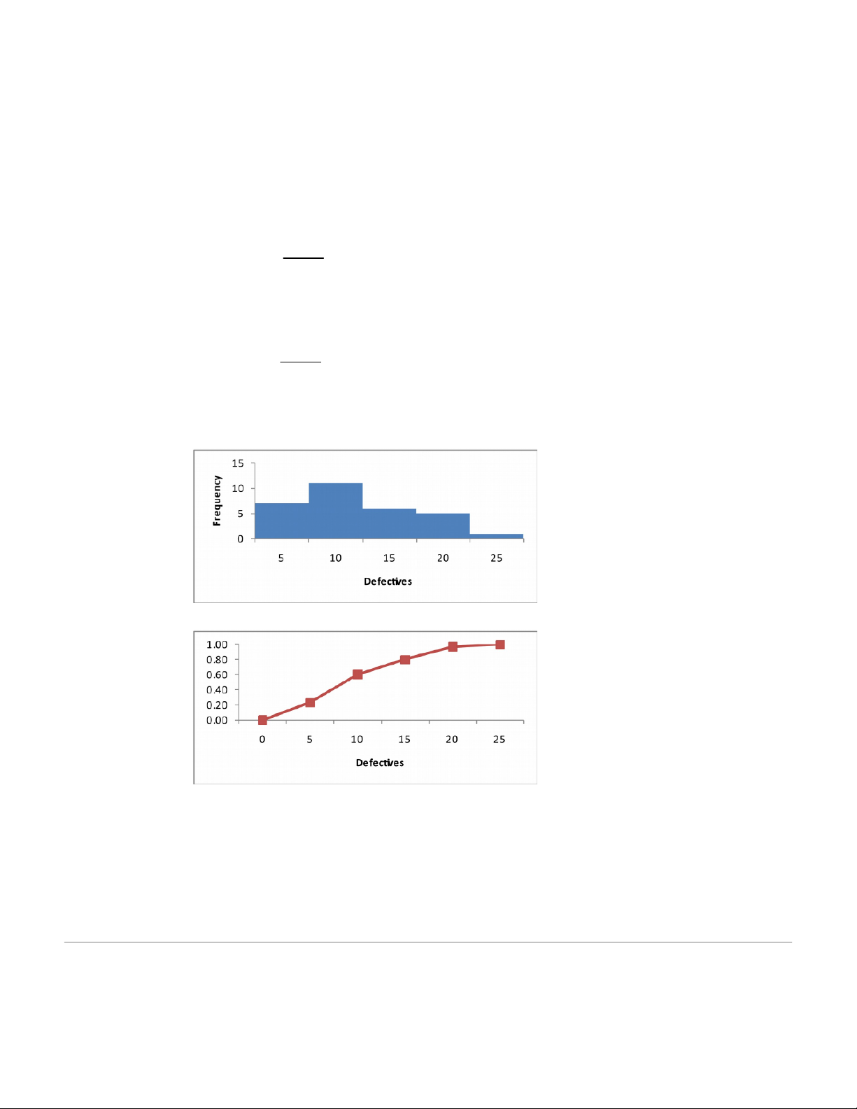
(rounded to .15); upper limits: 5.25, 5.40, 5.55, 5.70, 5.85, 6.00, 6.15 3.5a b
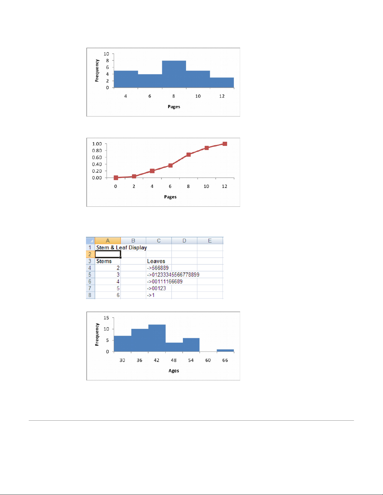
c The histogram is unimodal and somewhat positively skewed. 37 3.6 a b
c The number of pages is bimodal and slightly positively skewed. 3.7 a b 38 c
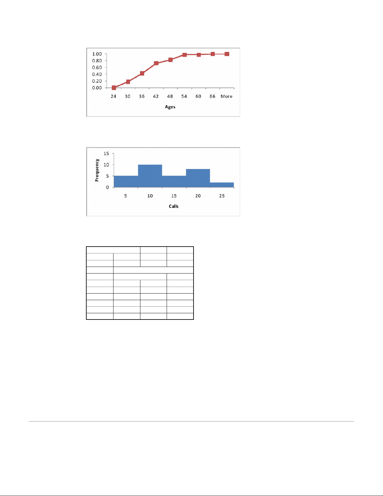
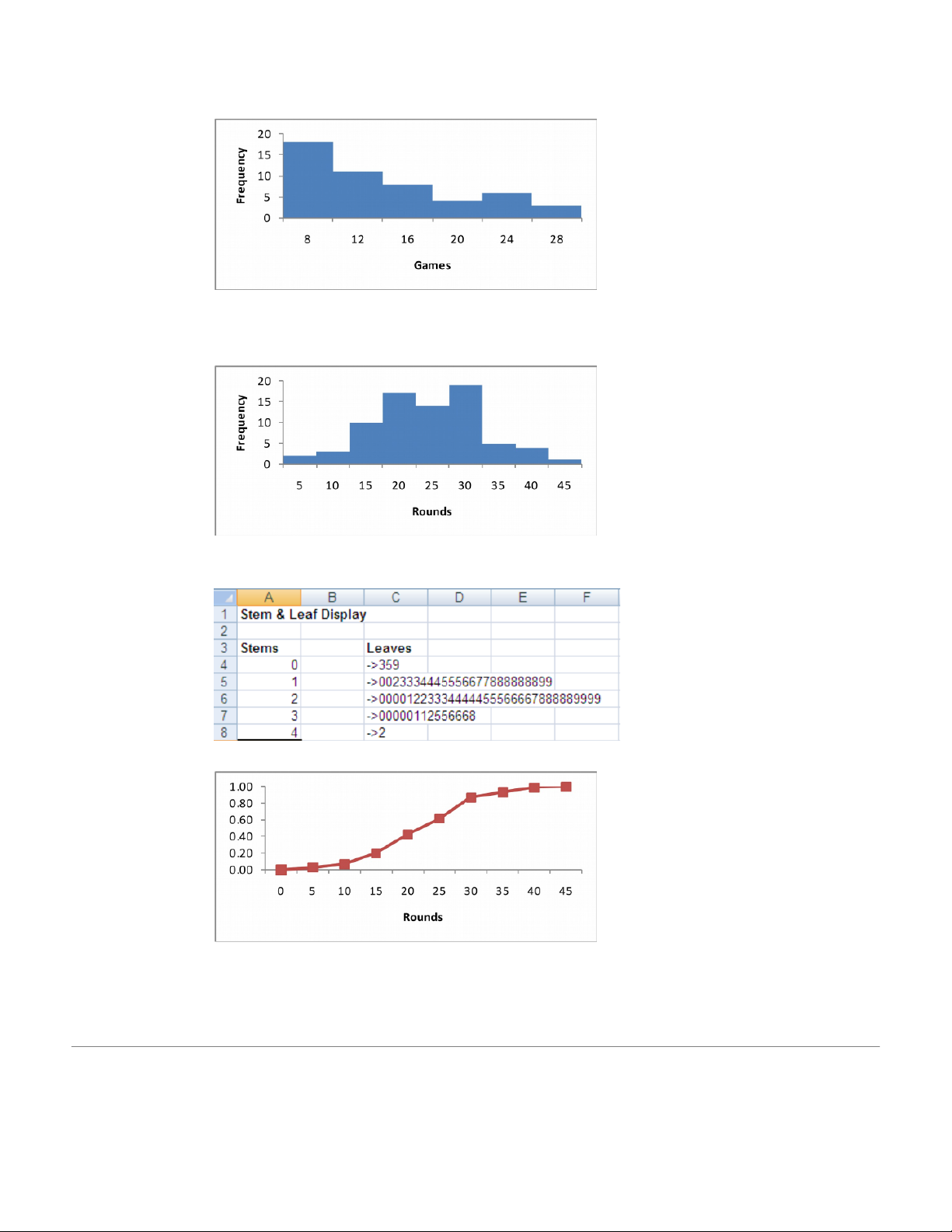
d The ages are bimodal and positively skewed. 3.8 The histogram is bimodal. 3.9 a Stem & Leaf Display Stems Leaves 30 ->0112222222356667777788 31 ->001113568 32 ->024777 33 ->0047 34 ->024455 35 ->7 36 ->7 37 ->9 39 b
c The histogram is positively skewed. 3.10 a b
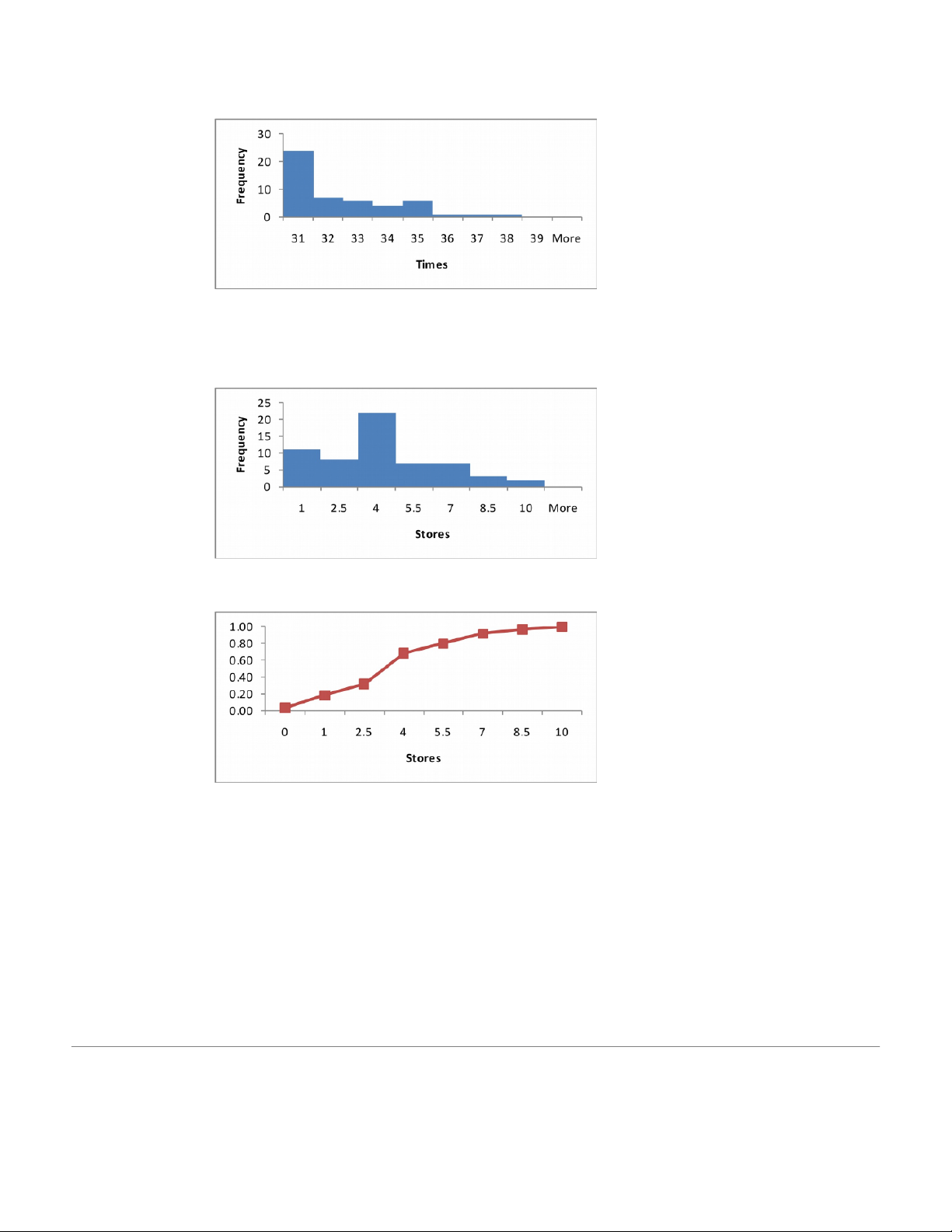
c The number of stores is bimodal and positively skewed. 40 3.11
The histogram is positively skewed. 3.12 a b c 41
d The histogram is symmetric (approximately) and bimodal. 3.13
The histogram is symmetric, unimodal, and bell shaped. 3.14 a b 42 c
d The histogram is slightly positively skewed, unimodal, and not bell-shaped. 3.15
The histogram is unimodal and positively skewed.
3.16 a The histogram should contain 9 or 10 bins. We chose 10. b
c The histogram is positively skewed.
d The histogram is not bell-shaped. 43 3.17
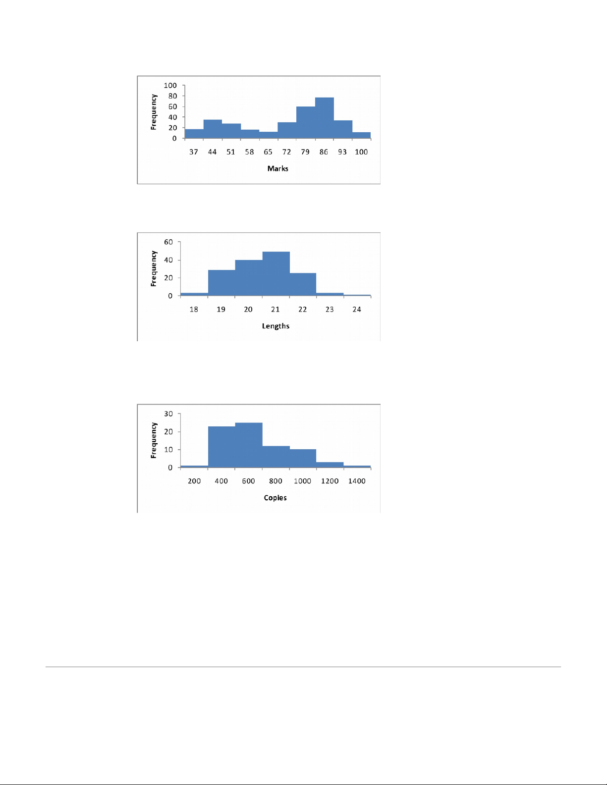
The histogram is negatively skewed, bimodal, and not bell shaped. 3.18
The histogram is unimodal, bell-shaped and roughly symmetric. Most of the lengths lie between 18 and 23 inches. 3.19
The histogram is unimodal and positively skewed. On most days the number of copies made is
between 200 and 1000. On a small percentage of days more than 1000 copies are made. 44 3.20
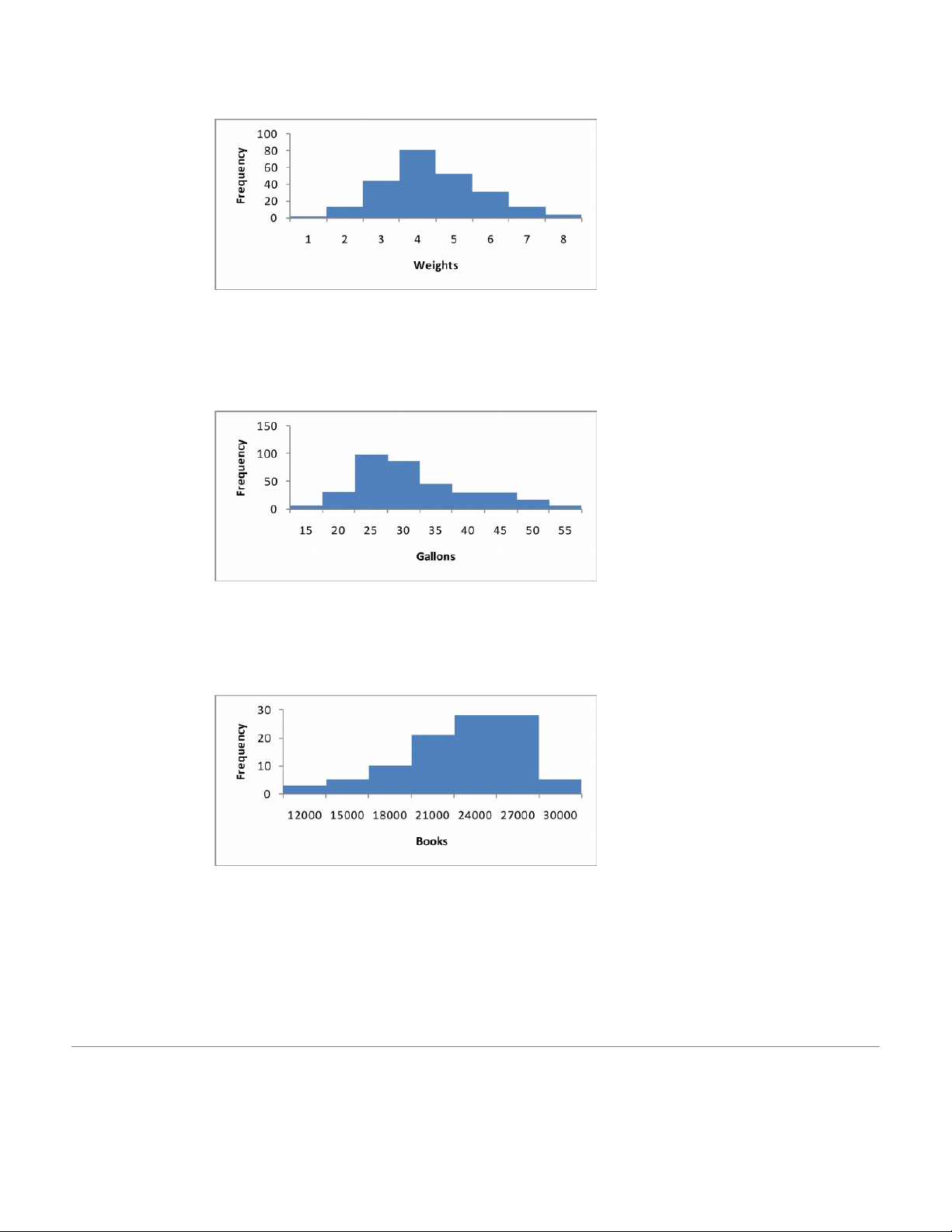
The histogram is unimodal, symmetric and bell-shaped. Most tomatoes weigh between 2 and 7
ounces with a small fraction weighing less than 2 ounces or more than 7 ounces. 3.21
The histogram is positively skewed and unimodal. Most households use between 20 and 45
gallons per day. The center of the distributions appears to be around 25 to 30 gallons. 3.22
The histogram of the number of books shipped daily is negatively skewed. It appears that there is
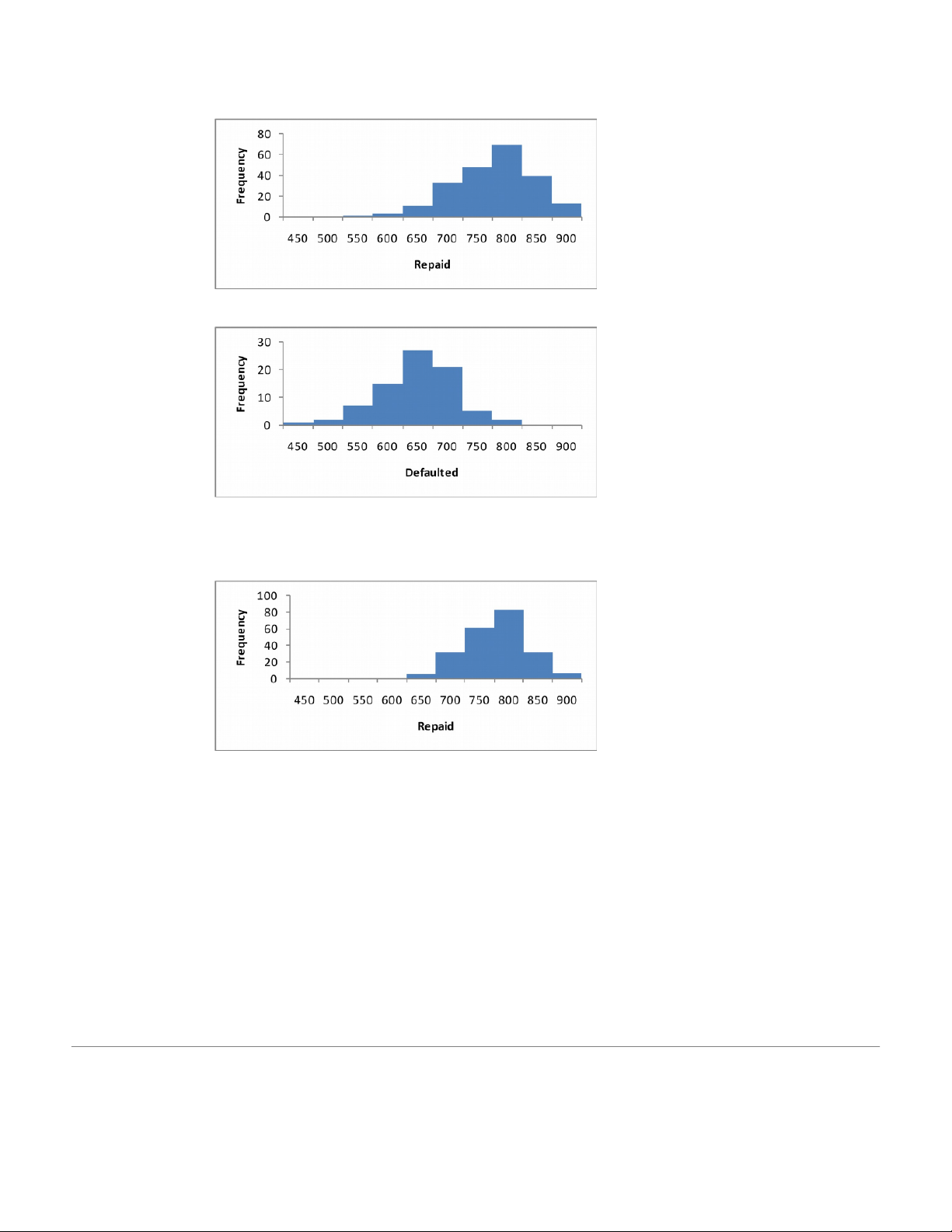
a maximum number that the company can ship. 45 3.23 a b
c The scorecards appear to be relatively poor predictors. 3.24 a 46 b
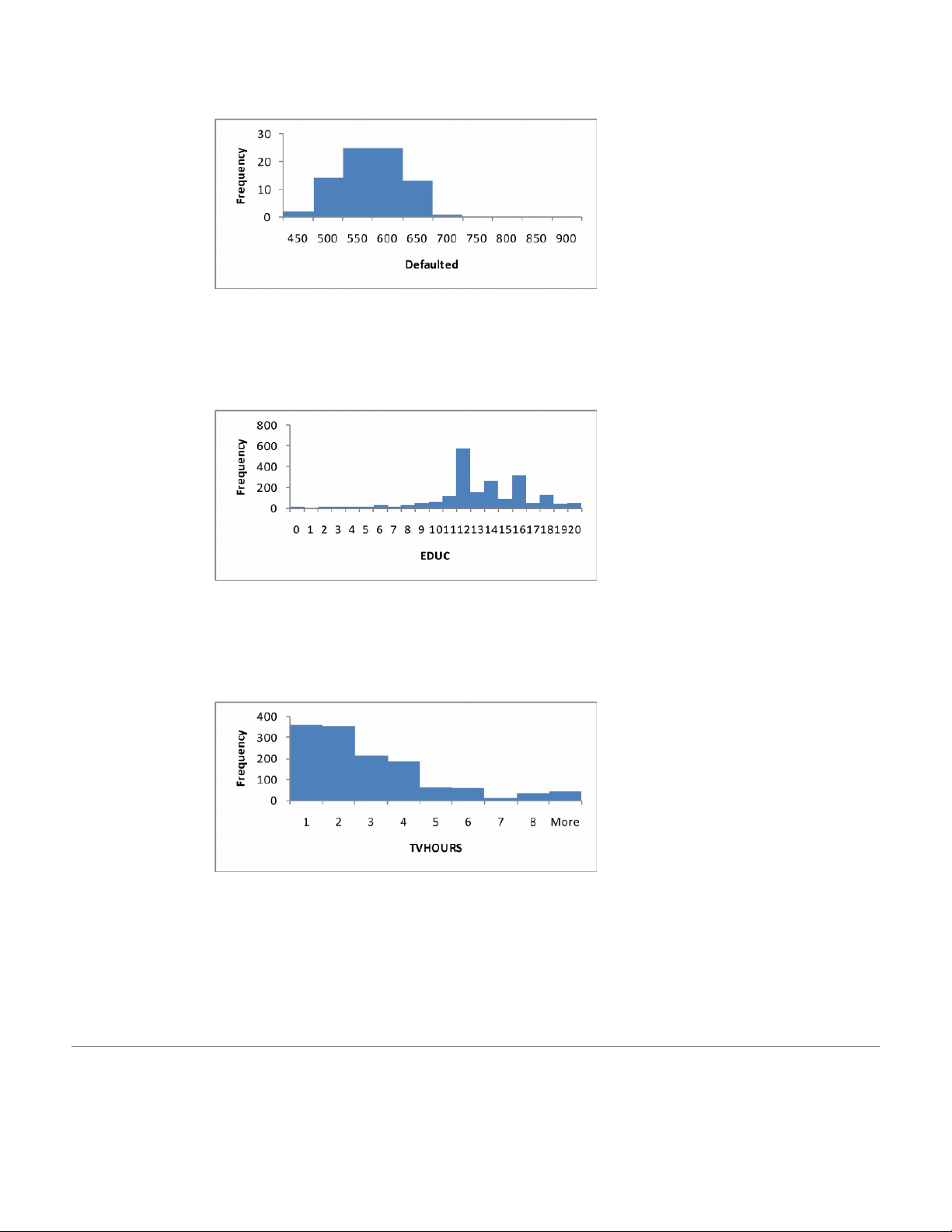
c. and d. This scorecard is a much better predictor. 3.25a Interval b
c The peaks in the histogram represent high school graduates , two-year college graduates, and university graduates. 3.26
The histogram is highly positively skewed indicating that most people watch 4 or less hours per
day with some watching considerably more. 47 3.27 3.28
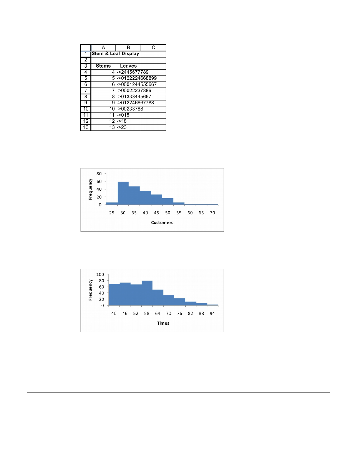
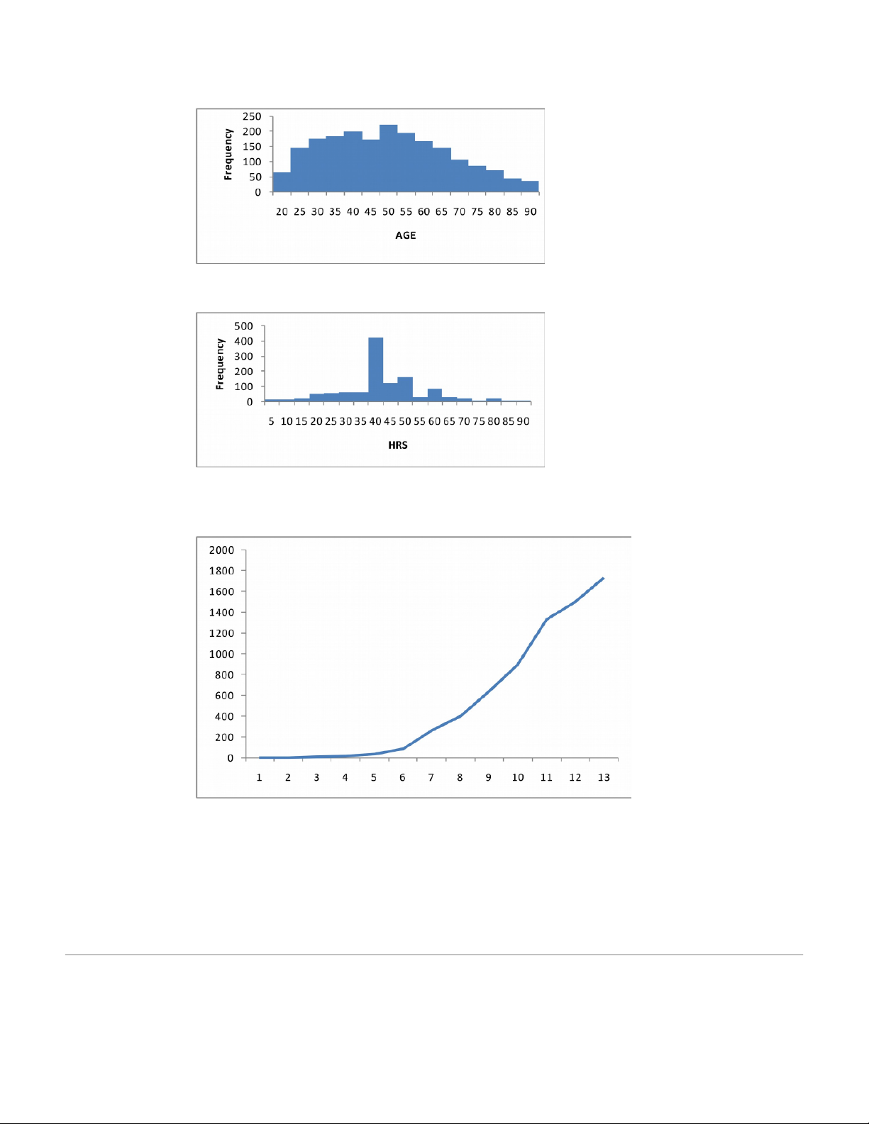
Many people work more than 40 hours per week. 3.29 48 3.30
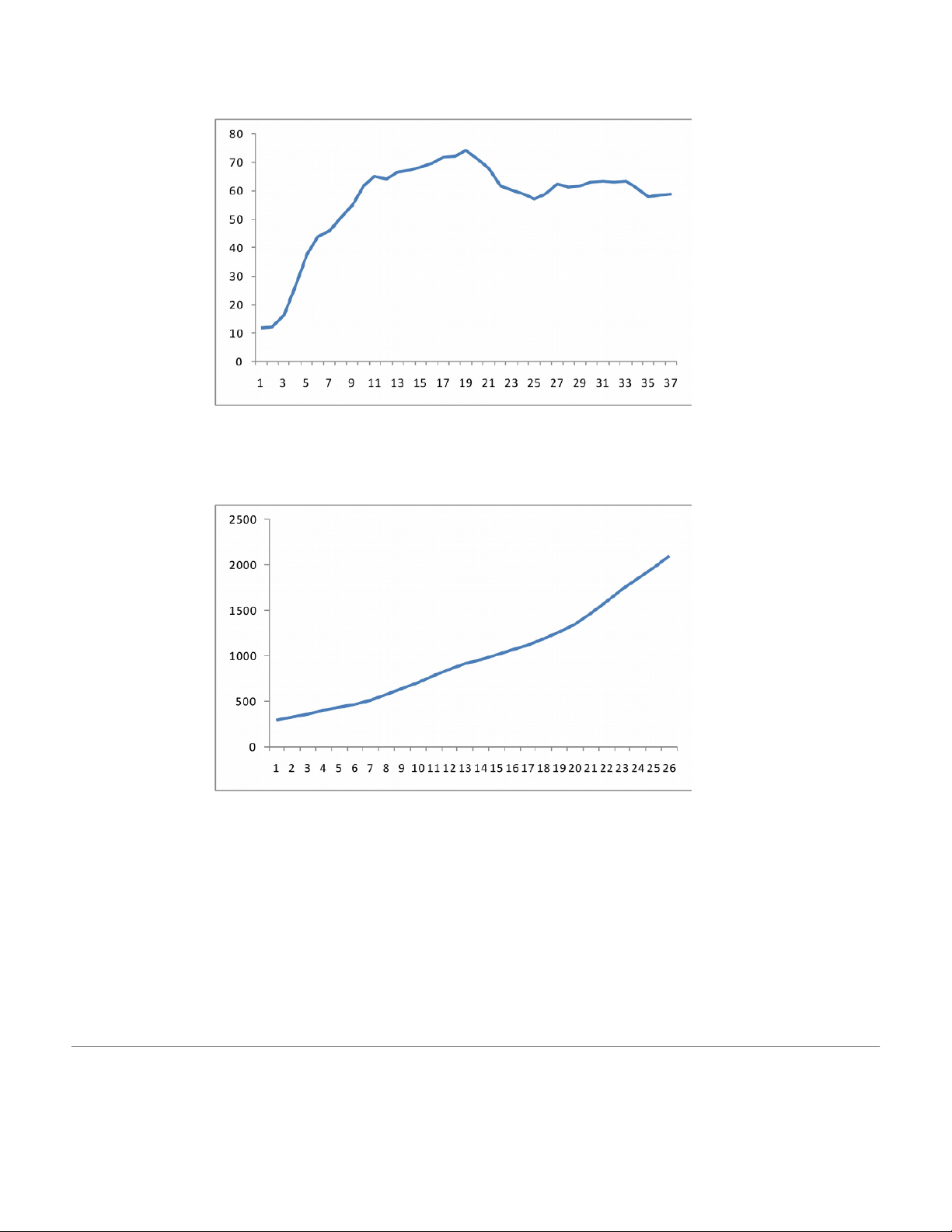
After a rapid increase the numbers have leveled off. 3.31
Total health care expenditures are rising faster than inflation 49 3.32
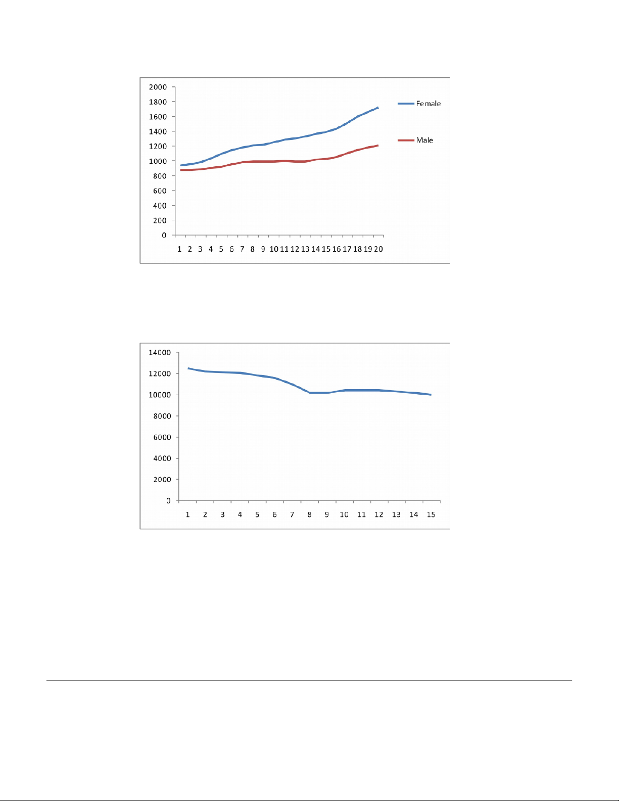
The numbers of females and males are both increasing with the number of females increasing faster. 3.33
The number of property crime decreased slowly over the 15 years. 50 3.34
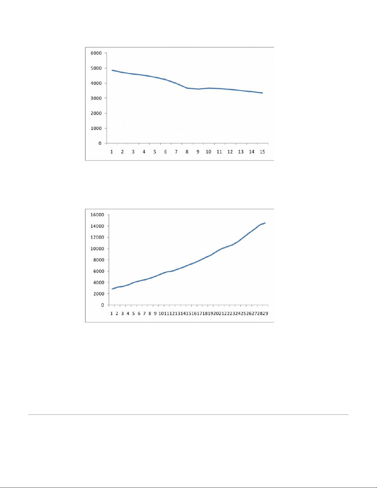
The per capita number of property crimes decreased faster than did the absolute number of property crimes. 3.35a
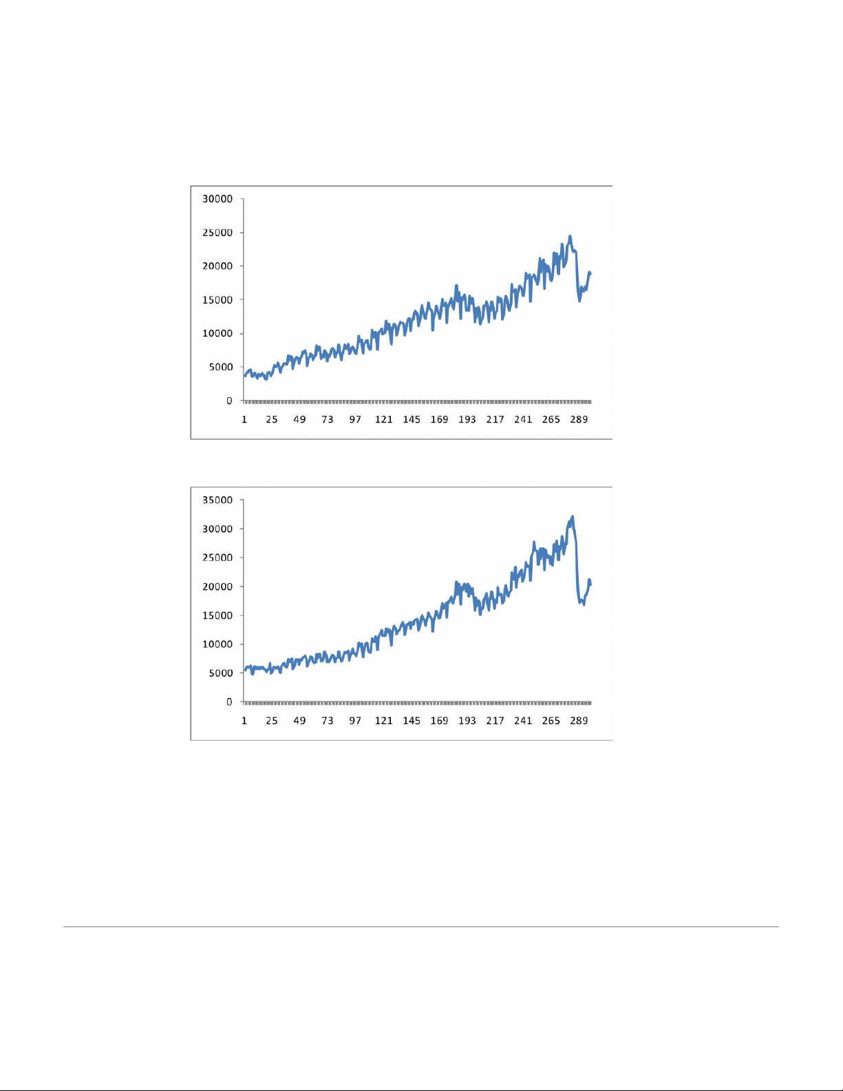
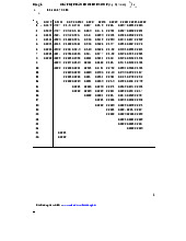
GDP increased rapidly over the 29 year period. 51 b
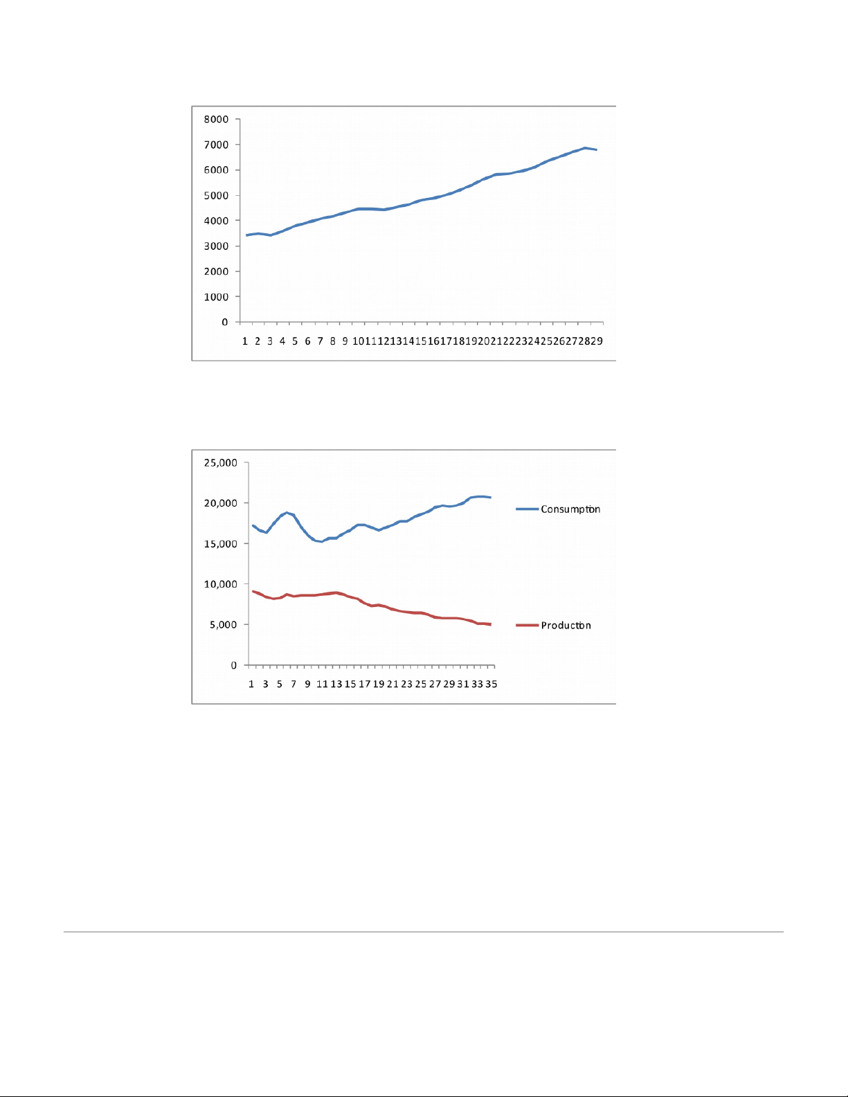
The inflation-adjusted GDP grew at a moderate rate. 3.36
Consumption is increasing and production is falling. 52 3.37
All areas as well as the whole country saw house prices staying ahead of inflation until the last three years. 3.38 53 b
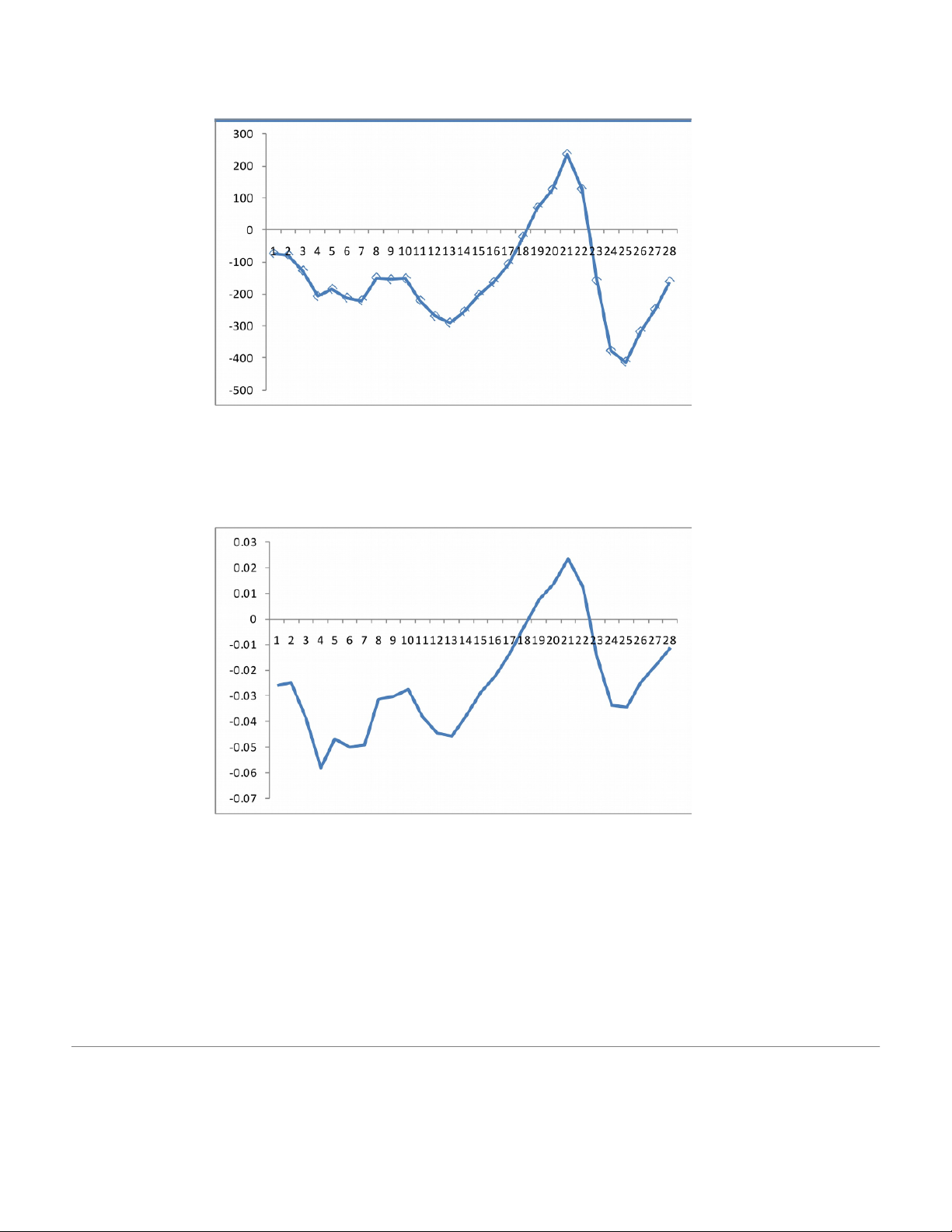
Over the last 28 years both receipts and outlays increased rapidly. There was a five-year period
where receipts were higher than outlays. Between 2004 and 2007 the deficit has decreased. 3.39
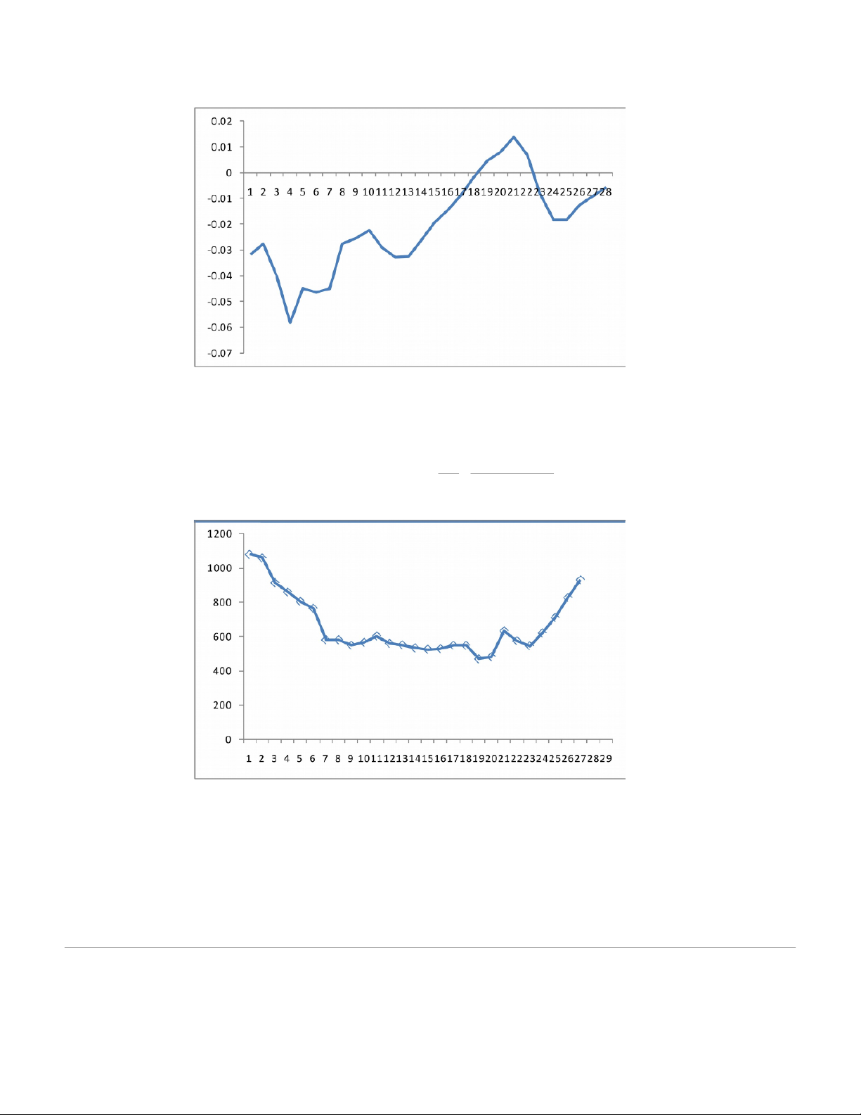
When the size of the economy as measured by GDP the deficits are not that large. 54 3.40
The inflation adjusted deficits are not large.
3.41 The cost is calculated as follows. Pr ice 100 Dis tan ce 000 , 1
Cost per year in 1982-84 dollars = CPI MPG 55
Even though the average distance travelled per year has increased the annual inflation-adjusted
cost of driving decreased from over $1,000 in 1980 to less than $600 in 2005 before starting to increase from 2002 to 2006. 3.42 Exports to Canada Imports from Canada 56