Chapter 5: Understanding Random Samples & Their Characteristics môn Xác suất thống kê| Trường Đại học Ngoại Thương

Lecturer: Nguyen Duong Nguyen, Mathematics Department, Faculty of Basic Science, FTU
Chapter 5. Sample theoretical basis 5.1. Concept of random sample
The set of al elements that have the same number of properties need to be studied is cal ed a population. Example.
a) When studying the height of youngsters in province A, we consider the population as
“The set of al youngsters of province A”.
b) When studying the defective product proportion of the company at a certain time, we
consider the population as “The set of al products of company B” (at that time).
The number of al elements of the population is cal ed the size of the population, denoted by N.
The characteristics of the population that need to be studied, for example: the
height of youngsters in province A or the "defective product " sign of company B.... These
are cal ed the research signs. We often denote the research sign by a random variable, such as X.
When the studied population is too large or the low level of reliability of the
survey data makes the calculation both difficult and expensive but stil does not get
accurate results, especial y when the size of the population is unknown (and N must be
considered to be infinite), it is practically impossible to study the whole population.
Therefore, people often apply the sample method: From the population, select n elements
and focus on studying these elements only. Based on that, conclusions can be drawn
about the signs that need to be studied in the population. This set of n elements is cal ed a sample of size n.
Definition. Let random variable X. Make n independent observations about the random
variable X. Let X be the random variable obtained when making the ith observation i
about the random variable X. Then, (X1, X2, …, Xn) is cal ed a random sample of size n
formed (or drawn) from the original random variable X, written W = (X1, X2 ,..., Xn). 1
Lecturer: Nguyen Duong Nguyen, Mathematics Department, Faculty of Basic Science, FTU
Note. Let W = (X1, X2, …, Xn) be a random sample formed from the original random
variable X. Then, X1, X2, ..., Xn are independent random variables and have the same
probability distribution as the original random variable X. Therefore, their characteristic
parameters are equal to the characteristic parameters of X:
E(X1) = E(X2) = … = E(Xn) = E(X)
V(X1) = V(X2) = … = V(Xn) = V(X)
If x1 is the observed outcome of random variable X1, x2 is the observed outcome of
the random variable X2, …, xn is the observed outcome of the random variable Xn, the set
of n values x1, x2, ..., xn is cal ed a specific sample, writte w n x , x , ..., x . 1 2 n
Example. Considering the population: “The set of all youngsters of province A”. To
determine the average height of the young people in province A, let X be the height of
youngsters in province A, then X is considered the original random variable of the
population. The requirement of the problem is to determine E(X). Suppose from the
population, we choose a sample of size 5. First, l X et
b e the height of the ith youngster, i
i 1, 2,...,5, we get a random sample of size 5: W = (X1, X2, X3, X4, X5)
formed from the original random variable X.
If x1 = 168 cm, x2 = 170 cm, x3 = 173 cm, x4 = 174cm, x5 = 178 cm, we get a
specific sample: w = (168, 170, 173, 174, 178).
If x1 = 165 cm, x2 = 169 cm, x3 = 172 cm, x4 = 175cm, x5 = 180 cm, we get a
specific sample: w = (165, 169, 172, 175, 180).
Note. A random sample of size n is the set of n random variables, and a specific sample is
the set of n values observed when a trial is performed on the random sample.
5.2. The experimental frequency distribution table
Assume that from the population with the original random variable X, draw a
specific sample of size n: w = (x1, x2, …, xn). For those n specific values, we can col apse
them by aggregating the same values. Suppose the specific sample after col apsing is
(x(1), x(2), …, x(k)) (assume we have sorted the x(i) in ascending order, i.e. x( 1) < x(2) < …< 2
Lecturer: Nguyen Duong Nguyen, Mathematics Department, Faculty of Basic Science, FTU
x(k)), where the value x(1) appears n1 times, x(2) appears n2 times, …, x(k) appears nk times
in a particular sample (Note: n1 + n2 + … + nk = n). Then the specific value of the sample
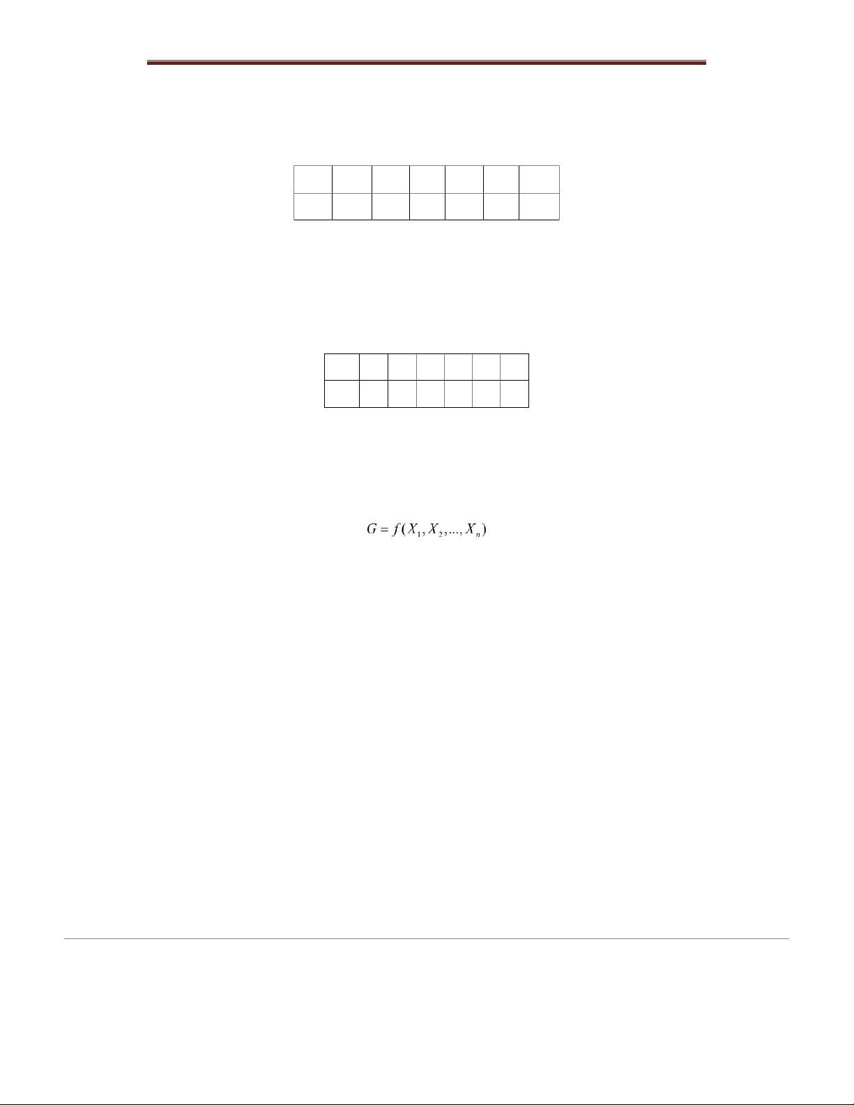
can be described the fol owing experimental frequency distribution table:
x(i) x(1) x(2) … x(i) … x(k) ni n1 n2 … ni … nk
Example. To investigate the waiting time of customers at a bank (unit: minutes), 10
people are randomly selected, the results are as fol ows: 9, 8, 10, 10, 12, 6, 11 , 10, 12, 8.
Make experimental distribution tables of the waiting time of customers.
Solution. The experimental frequency distribution table is xi 6 8 9 10 11 12 ni 1 2 1 3 1 2 5.3. Statistic
5.3.1. Definition. Suppose from the original random variable X in the population, draw a
random sample of size n: W = (X1, X2, …, Xn). A function f of the random variables
X , X , , X is cal ed a statistic, denoted by G. 1 2 n Note.
+) Since statistic is a function of random variables, it wil also be a random variable that
distributes some probability distribution and has characteristic parameters E(G), V(G).
+) If a random sample receives a specific value w , ( 1 x ,2x ,... n ,x ), G also takes a
specific value g = f(x1, x2, …, xn).
Meaning. Statistics with its probability distribution is the basis for generalizing the
information of the sample to the studied sign of the population.
5.3.2. Some characteristic statistics of random samples
Assuming that from the original random variable X in the population, draw a random sample of size n: W = (X1, X2, …, Xn) 3
Lecturer: Nguyen Duong Nguyen, Mathematics Department, Faculty of Basic Science, FTU
1) The sample mean S Trung Bình Mu Hàng
a) Definition: The sample mean is a statistic, denoted b Xy, which is the arithmetic mean of the sample values: Note.
+) When the random sample takes a specific value w = (x1, x2, …, xn) then the sample
mean also gets a specific value equal to: 1 n 1 k xx or x n x i n i n i 1 i 1 2 +) If 2 X ~ N ( , ) , ~ XN n ( , ) . +) If n > 30 and 2 E ( X ) m ;V ( ) X
, X has approximately normal distribution 2 ( Nm ,n ) .
b) The characteristic parameters of the sample mean: If the original random variable X has the expected v Ealu X e m and the variance 2 VX (m is also cal ed the
population mean, 2also known as the population variance), 2 E X ()m V ; X n () . 2) The mean squared deviation
a) Definition: The mean squared deviation is a statistic, denoted by MS, defined as: 11nn 22 2 MS i X X X X . nni 11
Note. When the random sample takes a specific value w = (x1, x2, …, xn) then the mean
squared deviation also takes a specific value equal to: 4
Lecturer: Nguyen Duong Nguyen, Mathematics Department, Faculty of Basic Science, FTU 1 n 2 1 k 2 ms x x or 2 2 ms n x x i n i n i 1 i 1
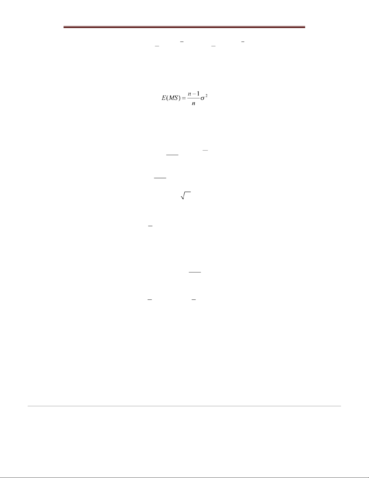
b) The characteristic parameter of the mean squared deviation I Vf 2 X () ,
3) The sample variance S2 and the variance S*2: a) Definition
● The sample variance is a statistic, denoted by S2, defined as: 1 n 2 2 S1 XX . i n i 1 n It is easy to see that: 2 S MS . n 1
The sample standard deviation: 2 SS .
● The variance S*2 is a statistic, defined as: *2 1 n 2 S X m , where i n E X () m . i 1
Note. When the random sample takes a specific value w = (x1, x2, …, xn) then the sample
variance S2 and the variance S*2 also take a specific value equal to: 2 n s ms , n 1 *2 11nk 22 s i x m n i ix m . nni 11
b) The characteristic parameter of S2 and *2 S VIf 2 X () , 22 E(S ) and *2 2 E(S ) . 5
Lecturer: Nguyen Duong Nguyen, Mathematics Department, Faculty of Basic Science, FTU
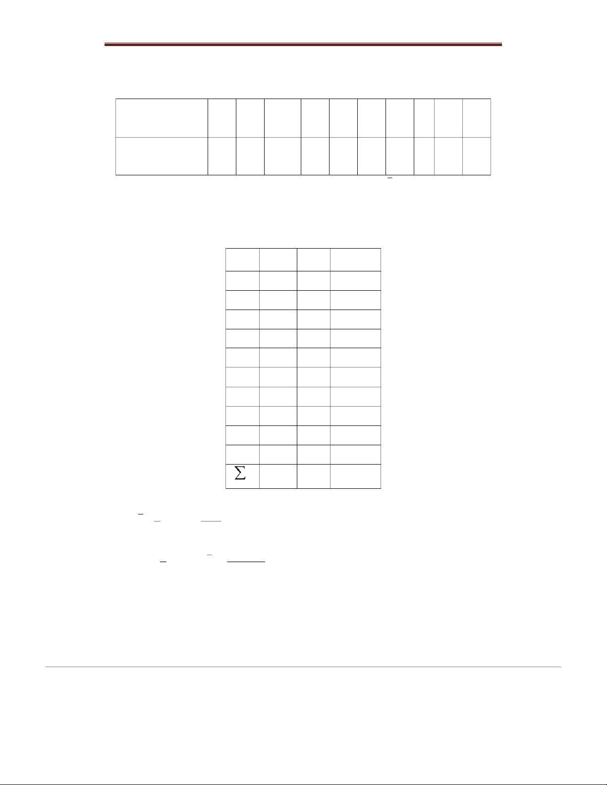
Example 1. Investigating monthly sales of 100 households trading in commodity A, we
obtain the fol owing table of data: Sales (mil ion
10.1 10.2 10.4 10.5 10.7 10.8 10.9 11 11.3 11.4 VND/month) Number of 2 3 8 13 25 20 12 10 6 1 households
Calculate sample characteristic values: the sample m x e , atn h e sample variance s2,
and the sample standard deviation s.
Solution. We make the fol owing table: xi ni nixi 2 nx i 10.1 2 20.2 204.02 10.2 3 30.6 312.12 10.4 8 83.2 865.28 10.5 13 136.5 1433.25 10.7 25 267.5 2862.25 10.8 20 216 2332.8 10.9 12 130.8 1425.72 11 10 110 1210 11.3 6 67.8 766.14 11.4 1 11 ,4 129.96 n=100 1074 11541.54 We have 1 1074 x n x 10.74 mil ion dong/month i n 100 1 11541.54 2 22 ms n x x 10.74 0.0678 i n 100 6
Lecturer: Nguyen Duong Nguyen, Mathematics Department, Faculty of Basic Science, FTU 2n 100 s ms
(0.0678) 0.0685 s = 0.2617 mil ion dong/month. n 1 99
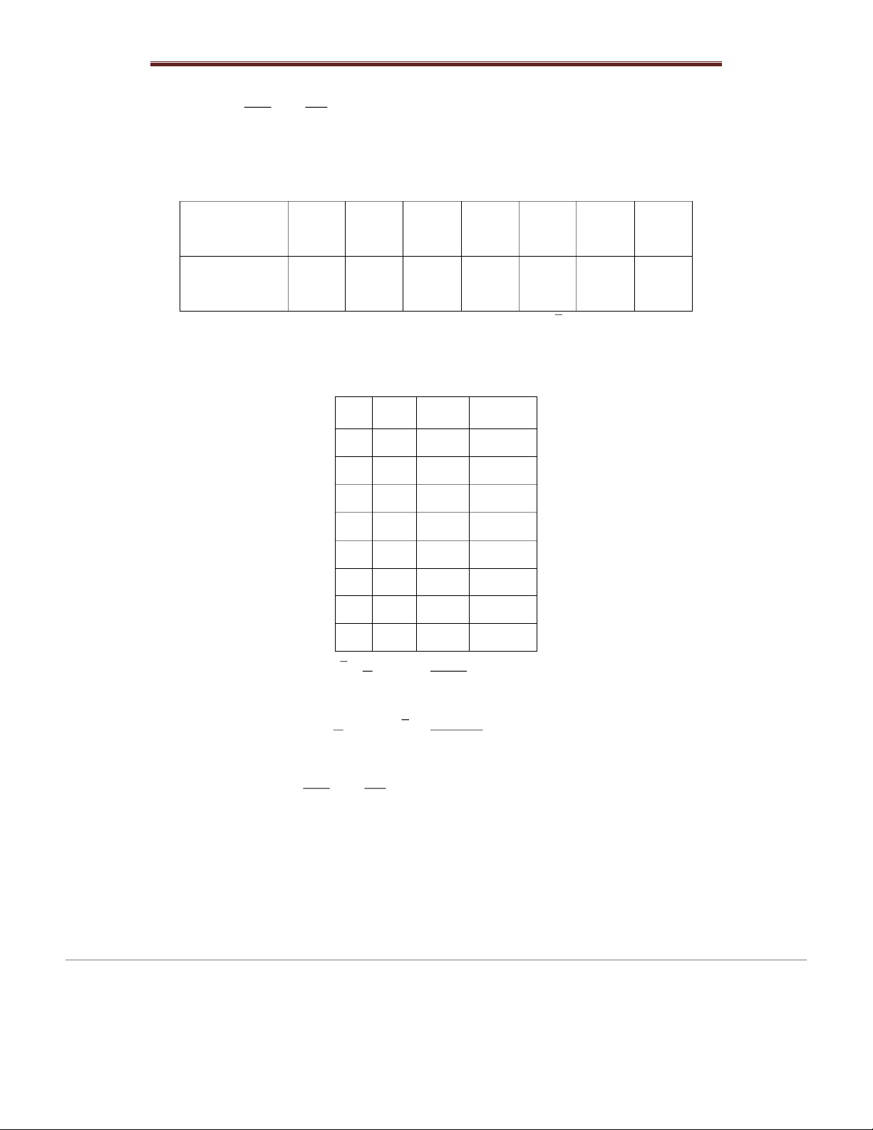
Example 2. Measuring the height of 100 young people aged from 18 to 22 years old in
province A, we obtain the fol owing data table: Height 154- 158- 162- 166- 170 - 174- 178- (unit: cm) 158 162 166 170 174 178 182 Number of 10 14 26 28 12 8 2 young people
Calculate the sample characteristics: the sample mxe,a tnh e sample variance s2
and the sample standard deviation s.
Solution. We make the fol owing table: xi ni nixi 2 nx i 156 10 1560 243360 160 14 2240 358400 164 26 4264 699296 168 28 4704 790272 172 12 2064 355008 176 8 1408 247808 180 2 360 64800 100 16600 2758944 1 16600 x n x 166 (cm) i n 100 1 2758944 2 22 ms n x x 166 33.44 i n 100 2n 100 s ms
(33.44) 33.7778 s = 5.8119 (cm) n 1 99 4) The sample proportion ly mu theo t l 7
Lecturer: Nguyen Duong Nguyen, Mathematics Department, Faculty of Basic Science, FTU
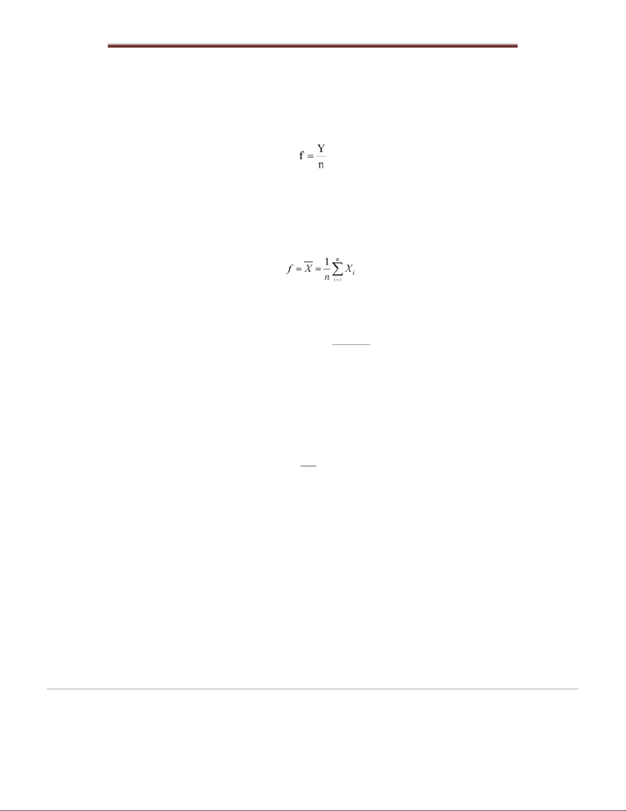
a) Definition: Assuming that from the original random variable X in the population,
draw randomly a sample of size n: W = (X1, X2, …, Xn), in which there are Y elements
with the studied sign (Y is also cal ed the number of successes in the sample). The
sample proportion is a statistic, denoted by f, defined as: Note.
+) On a specific sample, the sample proportion is a definite number.
+) If the original random variable X in the population distributes the zero-one
distribution, then the sample proportion is the sample mean:
b) The characteristic parameters of the sample proportion: If the original random
variable X has the zero-one distribution A(p) then () (1 ) E(f) = p; pp Vf n .
Example. Randomly checking 100 products produced by an automatic production line,
there are 40 defective products. Find the proportion of defective products of the given sample.
Solution. The proportion of defective products of the given sample is 40 f 0.4 100 8