Chapter 8 - large sample estimation in probability & statistics môn Xác suất thống kê| Trường Đại học Ngoại Thương
All values in the interval are possible values for the unknownpopulation parameter. 2. Any values outside the interval are unlikely to be the value of the unknown parameter. Tài liệu giúp bạn tham khảo, ôn tập và đạt kết quả cao. Mời đọc đón xem!
Môn: Xác suất thống kê (FTU) 355 tài liệu
Trường: Trường Đại học Ngoại Thương 1.1 K tài liệu
Tác giả:


Preview text:
318 ❍CHAPTER 8 LARGE-SAMPLE ESTIMATION CHAPTER REVIEW Key Concepts and Formulas I. Types of Estimators qˆ
1. Point estimator: a single number is calculated pp ˆ!z " a/2 % "pˆ & n
to estimate the population parameter. 2 s 2 m 1 " % " 2" 1 $m 2 (x
! 1 $x !2 ) !z a/2 %"s& &
2. Interval estimator: two numbers are calculated n1 n2
to form an interval that, with a certain amount ˆ ˆ p 1 q1 " % & "pˆ2q2" &
of confidence, contains the parameter. 1 $p 2 (pˆ1 $p ˆ2) !z a/2 %"pˆn n 1 2
II. Properties of Good Estimators
1. All values in the interval are possible values
1. Unbiased: the average value of the estimator
for the unknown population parameter.
equals the parameter to be estimated.
2. Any values outside the interval are unlikely to
2. Minimum variance: of all the unbiased estima-
be the value of the unknown parameter.
tors, the best estimator has a sampling distribu-
tion with the smallest standard error.
3. To compare two population means or propor-
tions, look for the value 0 in the confidence in-
3. The margin of error measures the maximum
terval. If 0 is in the interval, it is possible that
distance between the estimator and the true
the two population means or proportions are value of the parameter.
equal, and you should not declare a difference.
III. Large-Sample Point Estimators
If 0 is not in the interval, it is unlikely that the
two means or proportions are equal, and you
To estimate one of four population parameters when
can confidently declare a difference.
the sample sizes are large, use the following point
estimators with the appropriate margins of error. V. One-Sided Confidence Bounds Parameter Point Estimator 95% Margin of Error
Use either the upper (%) or lower ($) two- s
sided bound, with the critical value of z mx ! !1.96"" " $ # n! changed from za/2 to za. x qˆ VI. Choosing the Sample Size pp ˆ# "" " & n !1.96%"pˆn
1. Determine the size of the margin of error, B, 2
that you are willing to tolerate. s 2 m 1 " % " 2" 1 $m 2 x!1 $x!2 !1.96%"s& & n1 n2
2. Choose the sample size by solving for nor x x pˆ qˆ pˆ qˆ
n#n 1 #n 2 in the inequality: za/2 & SE 'B, p (pˆ 1 " $ "2" 1 1 " % 2 2 " 1 $p 2 1 $p ˆ2) #"" & "& n n $!1.96%"n n
where SE is a function of the sample size n. 1 2 1 2
IV. Large-Sample Interval Estimators
3. For quantitative populations, estimate the popu-
To estimate one of four population parameters
lation standard deviation using a previously
when the sample sizes are large, use the following
calculated value of sor the range approxima- tion s'Range/4. interval estimators.
4. For binomial populations, use the conservative Parameter (1 $a)100% Confidence Interval
approach and approximate pusing the value s mx ! !z " a/2 "" $ p#.5. # n! Supplementary Exercises
8.84 State the Central Limit Theorem. Of what value
a. Give the point estimate of the population mean m
is the Central Limit Theorem in large-sample statisti-
and find the margin of error for your estimate. cal estimation?
b. Find a 90% confidence interval for m. What does
8.85 A random sample of n#64 observations has a “90% confident” mean?
mean x! #29.1 and a standard deviation s#3.9. SUPPLEMENTARY EXERCISES ❍319
c. Find a 90% lower confidence bound for the popu-
include in the samples? Assume that the sample sizes
lation mean m. Why is this bound different from are equal.
the lower confidence limit in part b?
8.93 Does it Pay to Haggle? In Exercise 8.60, a
d. How many observations do you need to estimate m
survey done by Consumer Reports indicates that you
to within .5, with probability equal to .95?
should always try to negotiate for a better deal when
8.86 Independent random samples of n
shopping or paying for services.15 In fact, based on 1 #50 and n
their survey, 37% of the people under age 34 were
2 #60 observations were selected from populations
1 and 2, respectively. The sample sizes and computed
more likely to “haggle,” while only 13% of those 65
sample statistics are given in the table:
and older. Suppose that this survey included 72 people
under the age of 34 and 55 people who are 65 or older. Population a. What are the values of pˆ 12 1 and pˆ2 for the two groups in this survey? Sample Size 50 60
b. Find a 95% confidence interval for the difference Sample Mean 100.4 96.2 Sample Standard Deviation 0.8 1.3
in the proportion of people who are more likely to
“haggle” in the “under 34” versus “65 and older”
Find a 90% confidence interval for the difference in age groups.
population means and interpret the interval.
c. What conclusions can you draw regarding the
8.87 Refer to Exercise 8.86. Suppose you wish to groups compared in part b?
estimate (m1 $m 2) correct to within .2, with probabil-
8.94 Smoking and Blood Pressure An experiment
ity equal to .95. If you plan to use equal sample sizes, how large should n
was conducted to estimate the effect of smoking on the 1 and n2 be?
blood pressure of a group of 35 cigarette smokers, by
8.88 A random sample of n#500 observations from
taking the difference in the blood pressure readings at
a binomial population produced x#240 successes.
the beginning of the experiment and again 5 years
a. Find a point estimate for p, and find the margin of
later. The sample mean increase, measured in millime- error for your estimator.
ters of mercury, was x! #9.7, and the sample standard
b. Find a 90% confidence interval for p. Interpret this
deviation was s#5.8. Estimate the mean increase in interval.
blood pressure that one would expect for cigarette
smokers over the time span indicated by the experi-
8.89 Refer to Exercise 8.88. How large a sample is
ment. Find the margin of error. Describe the popula-
required if you wish to estimate pcorrect to within
tion associated with the mean that you have estimated.
.025, with probability equal to .90?
8.90 Independent random samples of n
8.95 Blood Pressure, continued Using a confidence 1 #40 and n
coefficient equal to .90, place a confidence interval on
2 #80 observations were selected from binomial
populations 1 and 2, respectively. The number of suc-
the mean increase in blood pressure for Exercise 8.94.
cesses in the two samples were x1 #17 and x 2 #23.
8.96 Iodine Concentration Based on repeated mea-
Find a 99% confidence interval for the difference
surements of the iodine concentration in a solution, a
between the two binomial population proportions.
chemist reports the concentration as 4.614, with an Interpret this interval. “error margin of .006.”
8.91 Refer to Exercise 8.90. Suppose you wish to esti-
a. How would you interpret the chemist’s “error
mate (p1 $p 2 ) correct to within .06, with probability margin”?
equal to .99, and you plan to use equal sample sizes—
b. If the reported concentration is based on a random
that is, n1 #n 2. How large should n1 and n2 be?
sample of n#30 measurements, with a sample
8.92 Ethnic Cuisine Ethnic groups in America buy
standard deviation s#.017, would you agree that
differing amounts of various food products because of
the chemist’s “error margin” is .006?
their ethnic cuisine. A researcher interested in market
8.97 Heights If it is assumed that the heights of men
segmentation for Asian and Hispanic households
are normally distributed with a standard deviation of
would like to estimate the proportion of households
2.5 inches, how large a sample should be taken to be
that select certain brands for various products. If the
fairly sure (probability .95) that the sample mean does
researcher wishes these estimates to be within .03 with
not differ from the true mean (population mean) by
probability .95, how many households should she
more than .50 in absolute value?
320 ❍CHAPTER 8 LARGE-SAMPLE ESTIMATION
8.98 Chicken Feed An experimenter fed different
a. This survey was based on “telephone interviews
rations, A and B, to two groups of 100 chicks each.
conducted with a nationally representative sample
Assume that all factors other than rations are the same
of 2250 adults, ages 18 years and older, living in
for both groups. Of the chicks fed ration A, 13 died,
continental U.S. telephone households.” What
and of the chicks fed ration B, 6 died.
problems might arise with this type of sampling?
a. Construct a 98% confidence interval for the true
b. How accurate do you expect the percentages
difference in mortality rates for the two rations.
given in the survey to be in estimating the actual
b. Can you conclude that there is a difference in the
population percentages? ( HINT : Find the margin
mortality rates for the two rations? of error.)
8.99 Antibiotics You want to estimate the mean
c. If you want to decrease your margin of error to be
hourly yield for a process that manufactures an antibi-
±1%, how large a sample should you take?
otic. You observe the process for 100 hourly periods
8.102 Sunflowers In an article in the Annals of
chosen at random, with the results x! #34 ounces per
Botany, a researcher reported the basal stem diameters
hour and s#3. Estimate the mean hourly yield for the
of two groups of dicot sunflowers: those that were left
process using a 95% confidence interval.
to sway freely in the wind and those that were artifi-
8.100 Eating Too Much? Partly because of our
cially supported.20 A similar experiment was con-
addiction to fast food, the average American consumes
ducted for monocot maize plants. Although the authors
32.7 pounds of cheese, 14.0 pounds of ice cream, and
measured other variables in a more complicated exper-
drinks 48.8 gallons of soda each year, according to the
imental design, assume that each group consisted of
2010 Statistical Abstract of the United States.18 Suppose
64 plants (a total of 128 sunflower and 128 maize
that we test the accuracy of these reported averages by
plants). The values shown in the table are the sample
selecting a random sample of 40 consumers, and record-
means plus or minus the standard error.
ing the following summary statistics: Sunflower Maize Cheese Ice Cream Soda (lbs/yr) (lbs/yr) (gal/yr) Free-Standing 35.3 !.72 16.2 !.41 Supported 32.1 !.72 14.6 !.40 Sample Mean 33.1 11.4 49.1 Sample Standard Deviation 3.8 3.2 4.5
Use your knowledge of statistical estimation to com-
Use your knowledge of statistical estimation to estimate
pare the free-standing and supported basal diameters
the average per-capita annual consumption for these three for the two plants. Write a paragraph describing your
products. Does this sample cause you to support or to
conclusions, making sure to include a measure of the
question the accuracy of the reported averages? Explain. accuracy of your inference.
8.101 Fast Food! Even though we know it may not
8.103 Basketball Tickets In a regular NBA season,
be good for us, many Americans really enjoy their fast
each team plays 82 games, some at home and some on
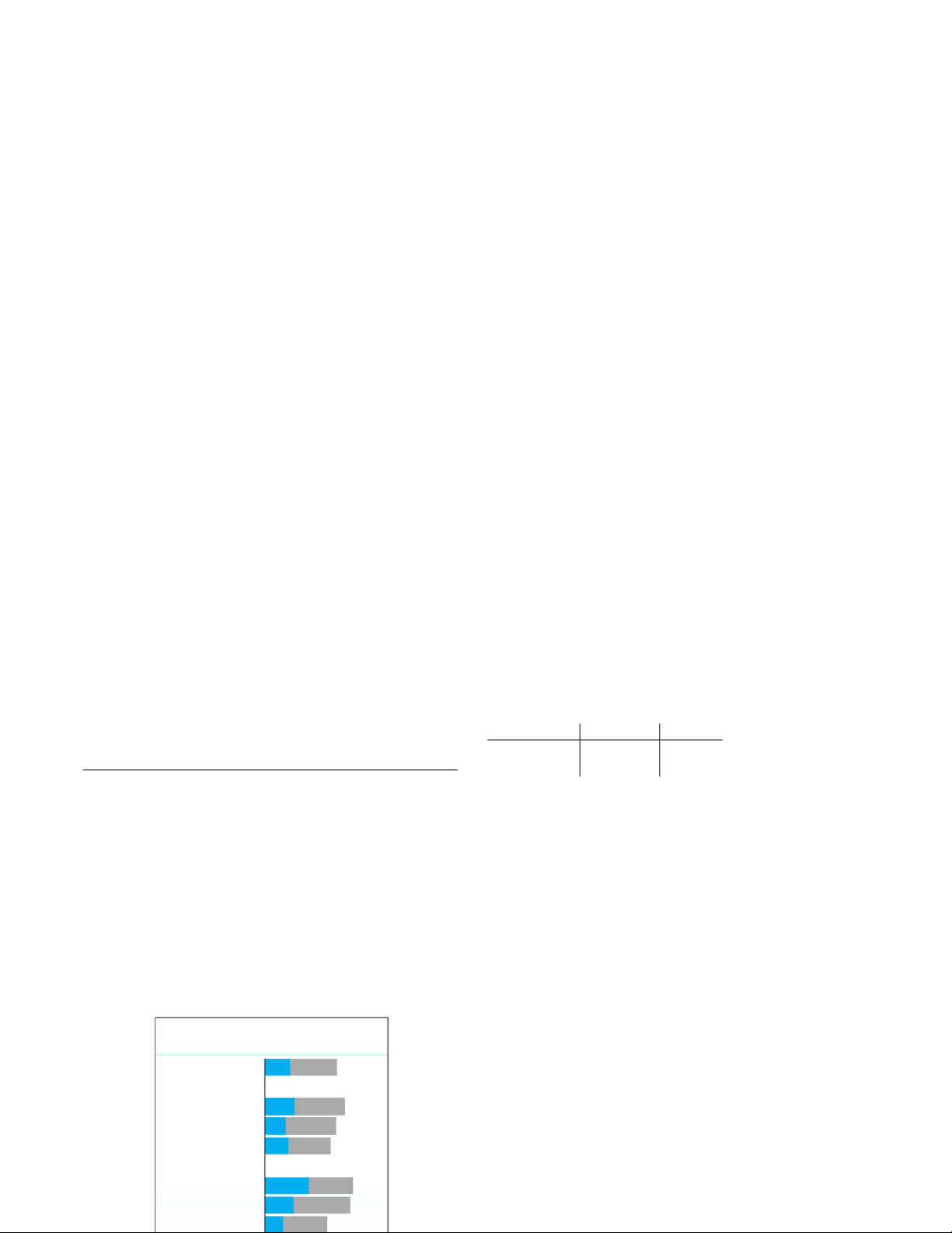
food! A survey conducted by Pew Research Center 19
the road. Can you afford the price of a ticket? The
graphically illustrated our penchant for eating out, and
Web site wiki.answers.com indicates that the low
in particular, eating fast food:
prices are around $10 for the high up seats while the
court-side seats are around $2000 to $5000 per game Percentage of Americans who
ìoften ” or “sometimes” overeat junk food
and that the average price of a ticket is $75.50 a
game.21 Suppose that we test this claim by selecting a All adults 19 36 55
random sample of n#50 ticket purchases from a Di D n i e n e o u o t u .t......
computer database and find that the average ticket 2+ times a week 23 38 61
price is $82.50 with a standard deviation of $75.25. 1 time a week 16 38 54 Less than weekly 18 32 50
a. Do you think that x, the price of an individual reg- or never
ular season ticket, has a mound-shaped distribu- Eat fast food... 2+ times a week 33 34 67
tion? If not, what shape would you expect? 1 time a week 22 43 65
b. If the distribution of the ticket prices is not normal, Less than weekly 14 34 48
you can still use the standard normal distribution to y or never Often Sometimes
construct a confidence interval for m, the average price of a ticket. Why?
Source: Pew Research Center, pewsocialtrends.org SUPPLEMENTARY EXERCISES ❍321
c. Construct a 95% confidence interval for m, the av-
a. Give the formula that you would use to construct a
erage price of a ticket. Does this confidence inter-
95% confidence interval for one of the population
val cause you support or question the claimed
means (e.g., mean time to skate the 6-meter
average price of $75.50? Explain. distance).
8.104 College Costs A dean of men wishes to esti-
b. Construct a 95% confidence interval for the mean
mate the average cost of the freshman year at a partic-
time to skate. Interpret this interval.
ular college correct to within $500, with a probability
8.109 Ice Hockey, continued Exercise 8.108 pre-
of .95. If a random sample of freshmen is to be
sented statistics from a study of fast starts by ice
selected and each asked to keep financial data, how
many must be included in the sample? Assume that the
hockey skaters. The mean and standard deviation of
the 69 individual average acceleration measurements
dean knows only that the range of expenditures will
vary from approximately $14,800 to $23,000.
over the 6-meter distance were 2.962 and .529 meters per second, respectively.
8.105 Quality Control A quality-control engineer
a. Find a 95% confidence interval for this population
wants to estimate the fraction of defectives in a large mean. Interpret the interval.
lot of printer ink cartridges. From previous experience,
b. Suppose you were dissatisfied with the width of
he feels that the actual fraction of defectives should be
this confidence interval and wanted to cut the inter-
somewhere around .05. How large a sample should he
val in half by increasing the sample size. How
take if he wants to estimate the true fraction to within
many skaters (total) would have to be included in
.01, using a 95% confidence interval? the study?
8.106 Circuit Boards Samples of 400 printed circuit
8.110 Ice Hockey, continued The mean and stan-
boards were selected from each of two production
dard deviation of the speeds of the sample of 69 skaters
lines A and B. Line A produced 40 defectives, and line
at the end of the 6-meter distance in Exercise 8.108
B produced 80 defectives. Estimate the difference in
were 5.753 and .892 meters per second, respectively.
the actual fractions of defectives for the two lines with
a. Find a 95% confidence interval for the mean
a confidence coefficient of .90.
velocity at the 6-meter mark. Interpret the interval.
8.107 Circuit Boards II Refer to Exercise 8.106.
b. Suppose you wanted to repeat the experiment and
Suppose 10 samples of n#400 printed circuit boards
you wanted to estimate this mean velocity correct
were tested and a confidence interval was constructed
to within .1 second, with probability .99. How
for pfor each of the 10 samples. What is the probabil-
many skaters would have to be included in your
ity that exactly one of the intervals will not contain the sample?
true value of p? That at least one interval will not con- tain the true value of p?
8.111 School Workers In addition to teachers and
administrative staff, schools also have many other
8.108 Ice Hockey G. Wayne Marino investigated
employees, including bus drivers, custodians, and cafe-
some of the variables related to “fast starts,” the accel-
teria workers. In Auburn, WA, the average hourly
eration and speed of a hockey player from a stopped
wage is $16.92 for bus drivers, $17.65 for custodians,
position.22 Sixty-nine hockey players, varsity and
and $12.86 for cafeteria workers.23 Suppose that a sec-
intramural, from the University of Illinois were
ond school district employs n#36 bus drivers who
included in the experiment. Each player was required
earn an average of $13.45 per hour with a standard
to move as rapidly as possible from a stopped position
deviation of s#$2.84. Find a 95% confidence interval
to cover a distance of 6 meters. The means and stan-
for the average hourly wage of bus drivers in school
dard deviations of some of the variables recorded for
districts similar to this one. Does your confidence
each of the 69 skaters are shown in the table:
interval enclose the Auburn, WA average of $16.92? Mean SD
What can you conclude about the hourly wages for bus Weight (kilograms) 75.270 9.470
drivers in this second school district? Stride Length (meters) 1.110 .205
8.112 Recidivism An experimental rehabilitation Stride Rate (strides/second) 3.310 .390
technique was used on released convicts. It was shown 2
Average Acceleration (meters/second )2.962 .529
that 79 of 121 men subjected to the technique pursued
Instantaneous Velocity (meters/second) 5.753 .892 Time to Skate (seconds) 1.953 .131
useful and crime-free lives for a 3-year period following
322 ❍CHAPTER 8 LARGE-SAMPLE ESTIMATION
prison release. Find a 95% confidence interval for p, the
8.115 Right- or Left-Handed A researcher classi-
probability that a convict subjected to the rehabilitation
fied his subjects as innately right-handed or left-
technique will follow a crime-free existence for at least
handed by comparing thumbnail widths. He took a 3 years after prison release.
sample of 400 men and found that 80 men could be
8.113 Specific Gravity If 36 measurements of the
classified as left-handed according to his criterion.
specific gravity of aluminum had a mean of 2.705 and
Estimate the proportion of all males in the population
a standard deviation of .028, construct a 98% confi-
who would test to be left-handed using a 95% confi-
dence interval for the actual specific gravity of dence interval. aluminum.
8.116 The Citrus Red Mite An entomologist
8.114 Audiology Research In a study to establish
wishes to estimate the average development time of
the absolute threshold of hearing, 70 male college
the citrus red mite correct to within .5 day. From pre-
freshmen were asked to participate. Each subject was
vious experiments it is known that sis approximately
seated in a soundproof room and a 150 H tone was
4 days. How large a sample should the entomologist
presented at a large number of stimulus levels in a
take to be 95% confident of her estimate?
randomized order. The subject was instructed to press
8.117 The Citrus Red Mite, continued A grower
a button if he detected the tone; the experimenter
believes that one in five of his citrus trees are infected
recorded the lowest stimulus level at which the tone
with the citrus red mite mentioned in Exercise 8.116.
was detected. The mean for the group was 21.6 db
How large a sample should be taken if the grower
with s#2.1. Estimate the mean absolute threshold for
wishes to estimate the proportion of his trees that are
all college freshmen and calculate the margin of error.
infected with citrus red mite to within .08? CASE STUDY How Reliable Is That Poll?
CBS News: How and Where America Eats
When Americans eat out at restaurants, most choose American food; however, tastes
for Mexican, Chinese, and Italian food vary from region to region of the United
States. In a recent CBS telephone survey 24 , it was found that 39% of families ate to-
gether 7 nights a week, slightly less than the 46% of families who reported eating
together 7 nights a week in an earlier survey by CBS. Most Americans, both men
and women, do some of the cooking when meals are cooked at home, as reported in
the following table where we compare the number of evening meals personally
cooked per week by men and women. Number of Meals Cooked 3 or Less 4 or More Men 76 24 Women 33 67
How often Americans eat out at restaurants is largely a function of income. “While
most households earning over $50,000 got restaurant food for dinner at least once in
the last week, 75% of those earning under $15,000 did not do so at all.” Income None 1–3 Nights 4 or More Nights All 47 49 4 Under $15,000 75 19 6 $15–$30,000 58 39 3 $30–$50,000 59 38 3 Over $50,000 31 64 5
In spite of all the negative publicity about obesity and high calories associated with p g p y y g
burgers and fries, many Americans continue to eat fast food to save time within busy schedules.
Tài liệu liên quan:
-
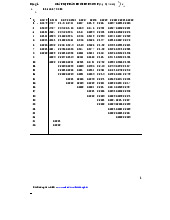
Bảng giá trị phân phối thống kê poisson và student môn Xác suất thống kê| Trường Đại học Ngoại Thương
27 14 -
Bảng giá trị quyết định thống kê wilcoxon rank-sum test môn Xác suất thống kê| Trường Đại học Ngoại Thương
30 15 -
Bài 1 Định nghĩa cổ điển về xác suất môn Xác suất thống kê| Trường Đại học Ngoại Thương
26 13 -
Exercises for probability & statistics môn Xác suất thống kê| Trường Đại học Ngoại Thương
26 13 -
Đề thi cuối kỳ lý thuyết môn Xác suất thống kê| Trường Đại học Ngoại Thương
27 14