Getting to Grips with Aircraft Performance - CRUISE môn Cơ học và tính năng tàu bay | Học viện Hàng Không Việt Nam

Getting to Grips with Aircraft Performance CRUISE
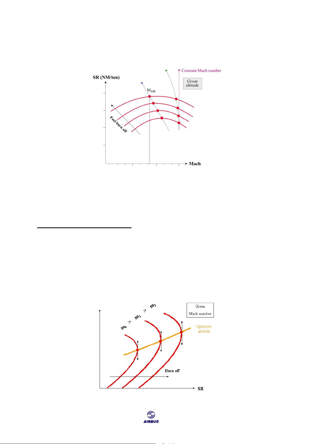
2.1.4. Constant Mach Number
The aircraft is often operated at a constant Mach number. MLRC
Figure F7: Constant Mach Number
Nevertheless, as the aircraft weight decreases, the gap between the selected
Mach and the MMR increases. As a result, fuel consumption increases beyond the optimum.
3. ALTITUDE OPTIMIZATION
3.1. Optimum Cruise Altitude
3.1.1. At a Constant Mach Number
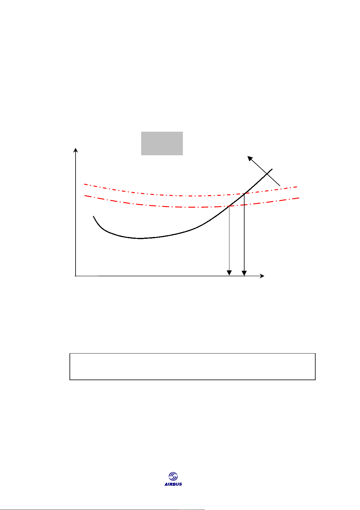
In examining SR changes with the altitude at a constant Mach number, it is
apparent that, for each weight, there is an altitude where SR is maximum. This
altitude is referred to as “optimum altitude” (see Figure F8). PA
Figure F8: Optimum Altitude Determination at Constant Mach Number 133 CRUISE
Getting to Grips with Aircraft Performance
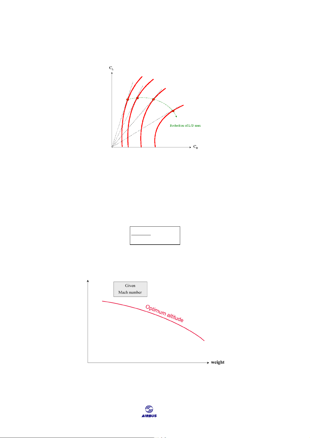
When the aircraft flies at the optimum altitude, it is operated at the maximum
lift to drag ratio corresponding to the selected Mach number (as in Figure F9). M < 0.76 M = 0.82 M = 0.84 M = 0.86
Figure F9: High Speed Polar Curve
When the aircraft flies at high speed, the polar curve depends on the indicated
Mach number, and decreases when Mach increases. So, for each Mach number,
there is a different value of (CL/CD)max, that is lower as the Mach number increases.
When the aircraft is cruising at the optimum altitude for a given Mach, CL is
fixed and corresponds to (CL/CD)max of the selected Mach number. As a result,
variable elements are weight and outside static pressure (Ps) of the optimum altitude.
The formula expressing a cruise at optimum altitude is: Weight = constant Ps
The optimum altitude curve, illustrated in Figure F10, is directly deduced from Figure F8. PA
Figure F10: Optimum Altitude and Weight at Constant Mach Number 134
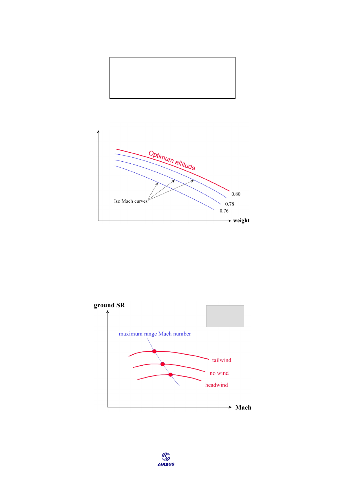
Getting to Grips with Aircraft Performance CRUISE Summary: a For given PA :  altitude optimum Ê  weight Ì ⇒   range specific Ê
ISO Mach number optimum altitude curves are all quasi-parallel (Figure F11). PA
Figure F11: ISO Mach Number Curves 3.1.2. Wind Influence
The MMR (or MLRC or MECON) value varies with headwind or tailwind, due to
changes in the ground SR. Figure F12 shows the Maximum Range Mach number versus wind variations. Given weight, PA
Figure F12: MMR and wind influence 135 CRUISE
Getting to Grips with Aircraft Performance As a result: Ground SR  Ê  tailwind ⇒ M  MR Ì Ground SR  Ì  headwind ⇒ M  Ê MR
The wind force can be different at different altitudes. For a given weight, when
cruise altitude is lower than optimum altitude, the specific range decreases (Figure
F8). Nevertheless, it is possible that, at a lower altitude with a favorable wind, the
ground specific range improves. When the favorable wind difference between the
optimum altitude and a lower one reaches a certain value, the ground-specific range
at lower altitude is higher than the ground-specific range at optimum altitude. As a
result, in such conditions, it is more economical to cruise at the lower altitude.
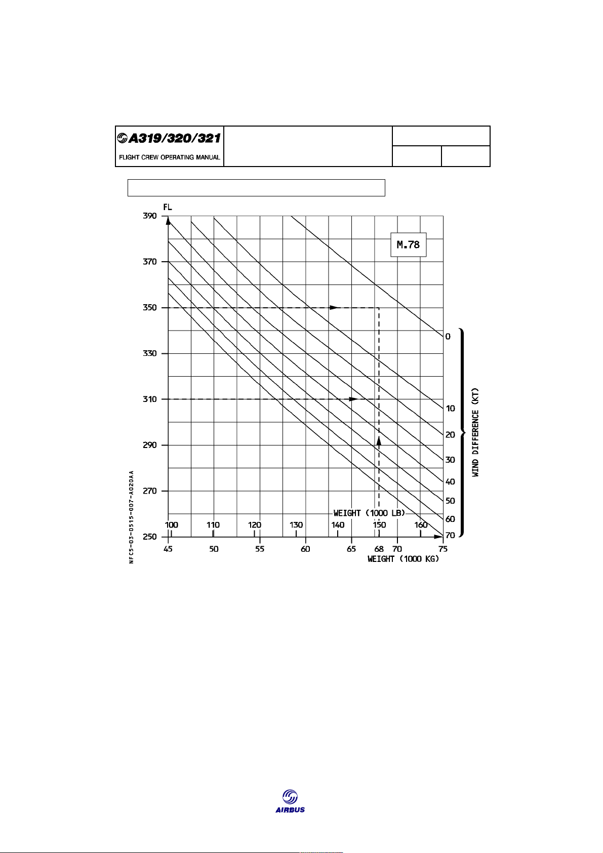
Figure F13 indicates the amount of favorable wind, necessary to obtain the
same ground-specific range at altitudes different from the optimum: 136
Getting to Grips with Aircraft Performance CRUISE IN FLIGHT PERFORMANCE 3.05.15 P 7 CRUISE SEQ 020 REV 24
WIND ALTITUDE TRADE FOR CONSTANT SPECIFIC RANGE GIVEN
: Weight : 68000 kg (150 000 lb) Wind at FL350 : 10 kt head FIND
: Minimum wind difference to descend to FL310 : (26 − 3) = 23 kt RESULTS
: Descent to FL310 may be considered provided the tail wind at this
altitude is more than (23 − 10) = 13 kt.
Figure F13: Optimum Altitude and Favorable Wind Difference 137 CRUISE
Getting to Grips with Aircraft Performance
3.2. Maximum Cruise Altitude
3.2.1. Limit Mach Number at Constant Altitude
Each engine has a limited Max-Cruise rating. This rating depends on the
maximum temperature that the turbines can sustain. As a result, when outside
temperature increases, maximum thrust decreases (see Figure F14). Thrust Given altitude Increasing weight drag m Max cruise thrust limit (ISA) (ISA + 15) Mach Mach2 Mach1
Figure F14: Influence of Temperature on Limit Mach Number at Given Altitude and Weight
Figure F14 illustrates the maximum possible Mach number, as a function of
temperature at a given altitude and weight.
The change in limit Mach number at constant altitude can, therefore, be summed up as:
For a given weight: Temperature Ò ⇒ Limit Mach number Ô
For a given temperature: Weight Ò ⇒ Limit Mach number Ô
3.2.2. Maximum Cruise Altitude
On the other hand, when an aircraft flies at a given Mach number, the higher
the altitude, the more the thrust must be increased. The maximum cruise altitude is
defined for a given weight, as the maximum altitude that an aircraft can maintain at
maximum cruise thrust when the pilot maintains a fixed Mach number. 138
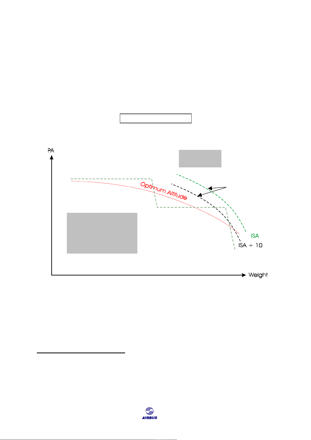
Getting to Grips with Aircraft Performance CRUISE . PA Non available area Given Mach under ISA conditions number PA2 PA1 ≤ ISA + 10 ISA + 20 weight m2 m1
Figure F15: Maximum Altitudes at Maximum Cruise Thrust
From Figure F15, it can be deduced that:
• At m1, the maximum altitude is PA1 for temperatures less than ISA + 10
• At m2, the maximum altitude is PA2 for temperatures less than ISA + 10, but
PA1 for temperatures equal to ISA + 20.
Maximum cruise altitude variations can be summed up as: weight Ê ⇒ Maximum cruise altitude Ì temperature Ê ⇒ maximum cruise altitude Ì Mach number Ê ⇒ maximum cruise altitude Ì
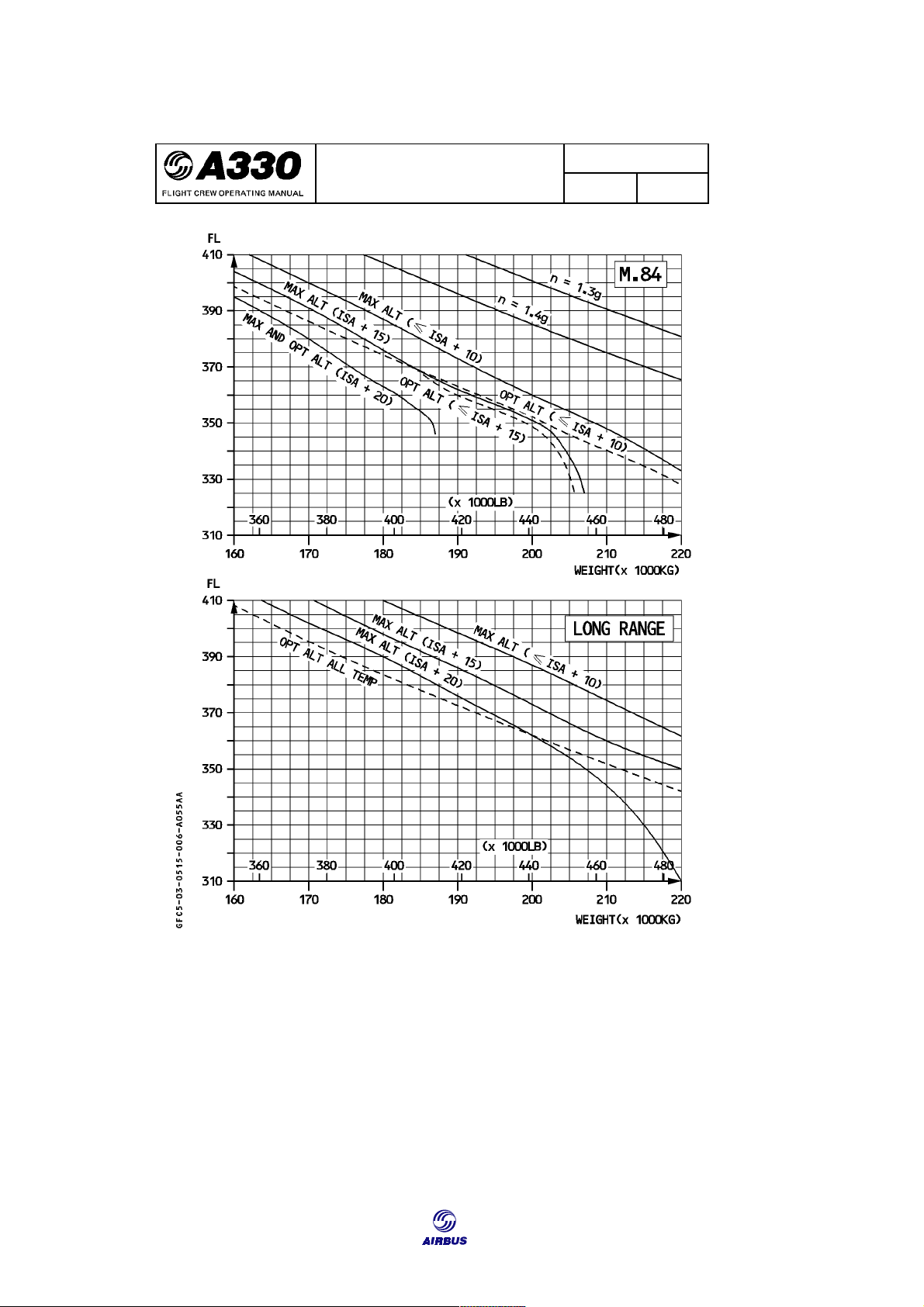
Figure F16 illustrates how maximum and optimum altitudes are shown in an A330 FCOM: 139 CRUISE
Getting to Grips with Aircraft Performance IN FLIGHT PERFORMANCE 3.05.15 P 6 CRUISE SEQ 055 REV 06
Figure F16: Maximum and Optimum Altitude 140
Getting to Grips with Aircraft Performance CRUISE
3.3. En route Maneuver Limits 3.3.1. Lift Range
In level flight, lift balances weight and, when CL equals CLmax, the lift limit is
reached. At this point, if the angle of attack increases, a stall occurs.
Lift limit equation: mg = 0.7 S P C M2 S Lmax CLmax M2 Drop of CLmax due to compressibility effects Flyable area Mach
Figure F17: CLmax M2 Curve versus Mach Number
At a given weight, depending on the lift limit equation, each CLmax.M2 value
corresponds to a static pressure (Ps) value. That is, a pressure altitude (PA).
Therefore, there is a direct relationship between CLmax.M2 and PA.
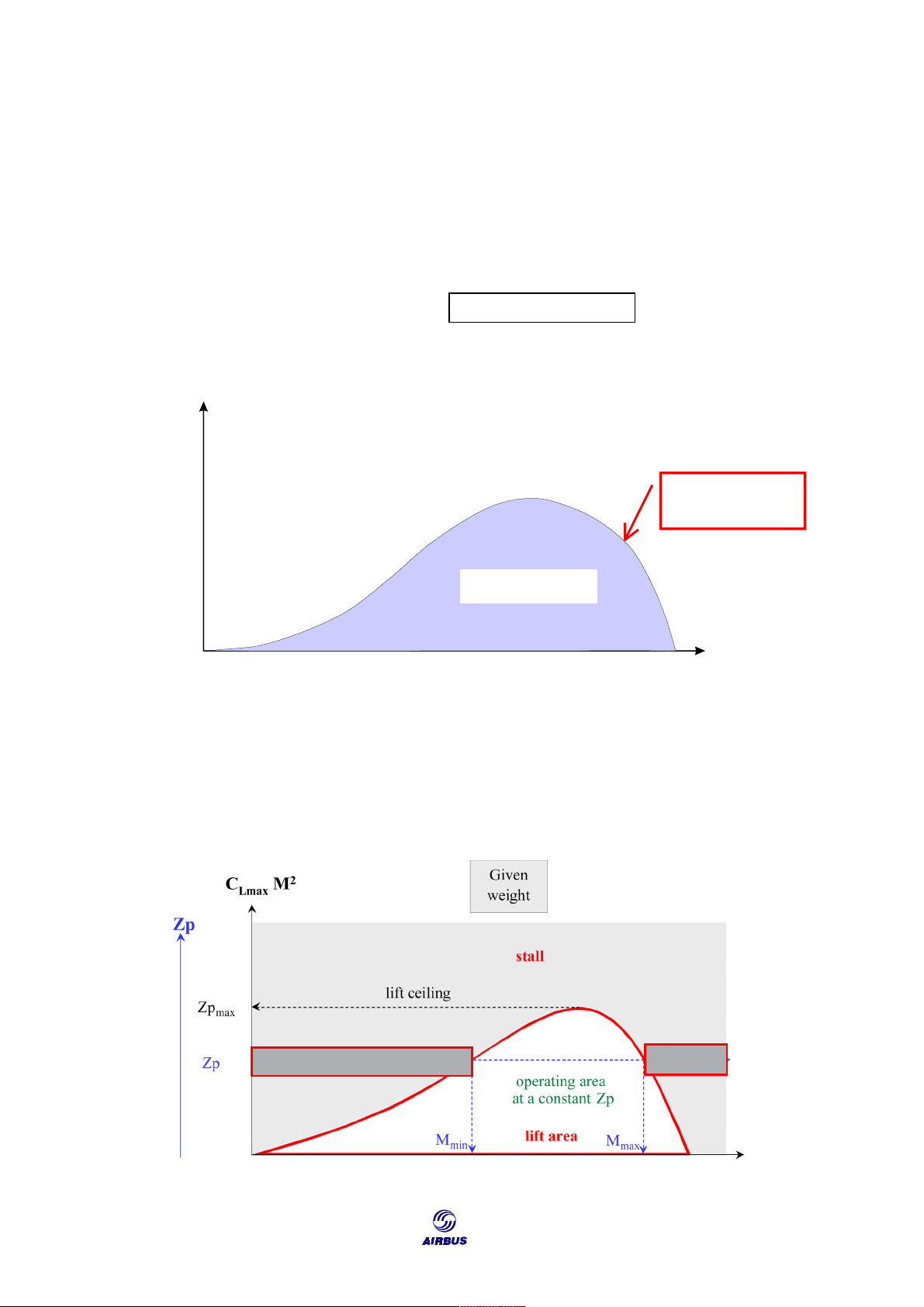
Figure F18 shows that, for a given PA, flight is possible between Mmin and
Mmax. When PA increases, the Mach range decreases until it is reduced to a single
point corresponding to the lift ceiling (PAmax). STALL STALL
Figure F18: Lift Area Definition 141 CRUISE
Getting to Grips with Aircraft Performance
3.3.2. Operating Maneuver Limitations 3.3.2.1. Buffet phenomenon
Concerning the low Mach number limit, when speed decreases, the angle of
attack must be increased in order to increase the lift coefficient, which keeps the forces balanced. Figure F19: Low Speed Stall
In any case, it is not possible to indefinitely increase the angle of attack (AoA).
At a high AoA, the airflow separates from the upper wing surface. If the AoA
continues to increase, the point of airflow separation is unstable and rapidly fluctuates
back and forth. Consequently, the pressure distribution changes constantly and also
changes the lift’s position and magnitude. This effect is cal ed buffeting and is
evidenced by severe vibrations.
When the AoA reaches a maximum value, the separation point moves further
ahead and total flow separation of the upper surface is achieved. This phenomenon
leads to a significant loss of lift, referred to as a stall.
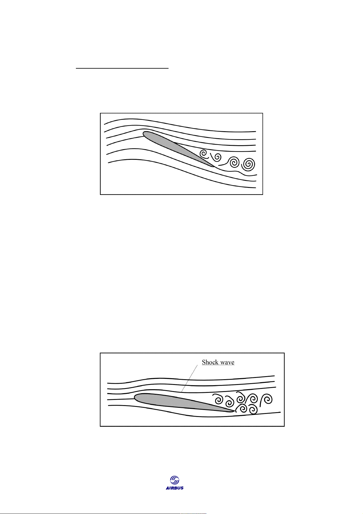
The high Mach number limit phenomenon is quite different. In fact, at high
speed, compressibility effects produce shock waves on the upper wing surface.
When Mach number, and/or AoA increase, the airflow separates from the upper
surface behind the shock wave, which becomes unstable and induces buffeting of the
same type as encountered in the low speed case. Figure F20: High Speed Airflow 142
Getting to Grips with Aircraft Performance CRUISE 3.3.2.2. Buffet limit
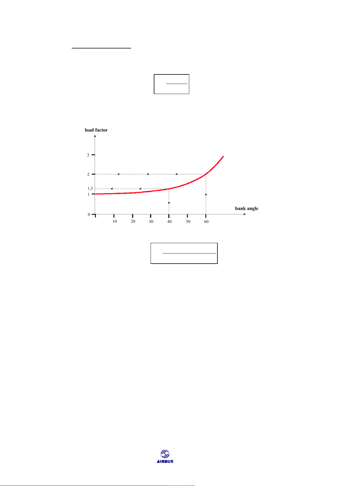
When maneuvering, the aircraft is subject to a load factor expressed as: Lift n = Weight
During turns, the load factor value mainly depends on the bank angle, as
shown in Figure F21. In fact, in level flight, n = 1/cos(bank angle).
Figure F21: Load Factor versus Bank Angle 0.7 S P C M2 At the lift limit, n S Lmax = m g
At a given pressure altitude (Ps) and given weight (mg), one load factor
corresponds to each CL max M2. Therefore, a curve representing load factor versus
Mach number will have the same shape as the one observed in Figure F17.
In fact, the useful limit Mach numbers in operation are the ones for which buffeting occurs.
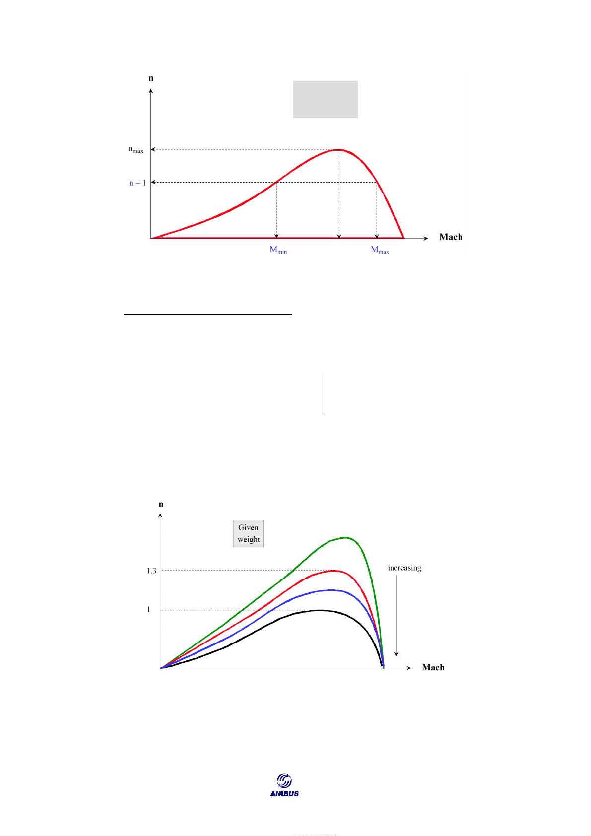
Figure F22 represents the buffet limit, and for n = 1 (level straight flight), a
minimum Mach appears for low speed buffet and a maximum Mach for high speed
buffet. When n increases, the Mach number range decreases, so that when n = n max, Mmin = Mmax.
So, nmax is the maximum admissible load factor at this weight and altitude, and
the corresponding Mach number M allows the highest margin regarding buffet limit. 143 CRUISE
Getting to Grips with Aircraft Performance Given Weight, PA M
Figure F22: Load Factor and Lift Area
3.3.2.3. Pressure altitude effect
Figure F23 illustrates the effects of pressure altitude on the lift area. It appears that, for a given weight: n max Ì Pressure altitude Ê lift range Ì
When nmax = 1, the aircraft has reached the lift ceiling. For example, in Figure
F23, PA3 corresponds to the lift ceiling at a given weight. PA0 PA1 PA PA2 PA3
Figure F23: Influence of Pressure Altitude on the Lift Limit
At pressure altitude PA1 (Figure F23), nmax = 1.3. That is to say, it is possible to
bear a load factor equal to 1.3, or make a 40° bank turn before buffeting occurs. 144
Getting to Grips with Aircraft Performance CRUISE
In order to maintain a minimum margin against buffeting and ensure good
aircraft maneuverability, it is necessary to determine an acceptable load factor limit
below which buffeting shall never occur. This load factor limit is generally fixed to
1.3. This value is an operating limitation, but not a regulatory one. The corresponding
altitude is called the “1.3g buffet limited altitude” or “buffet ceiling”.
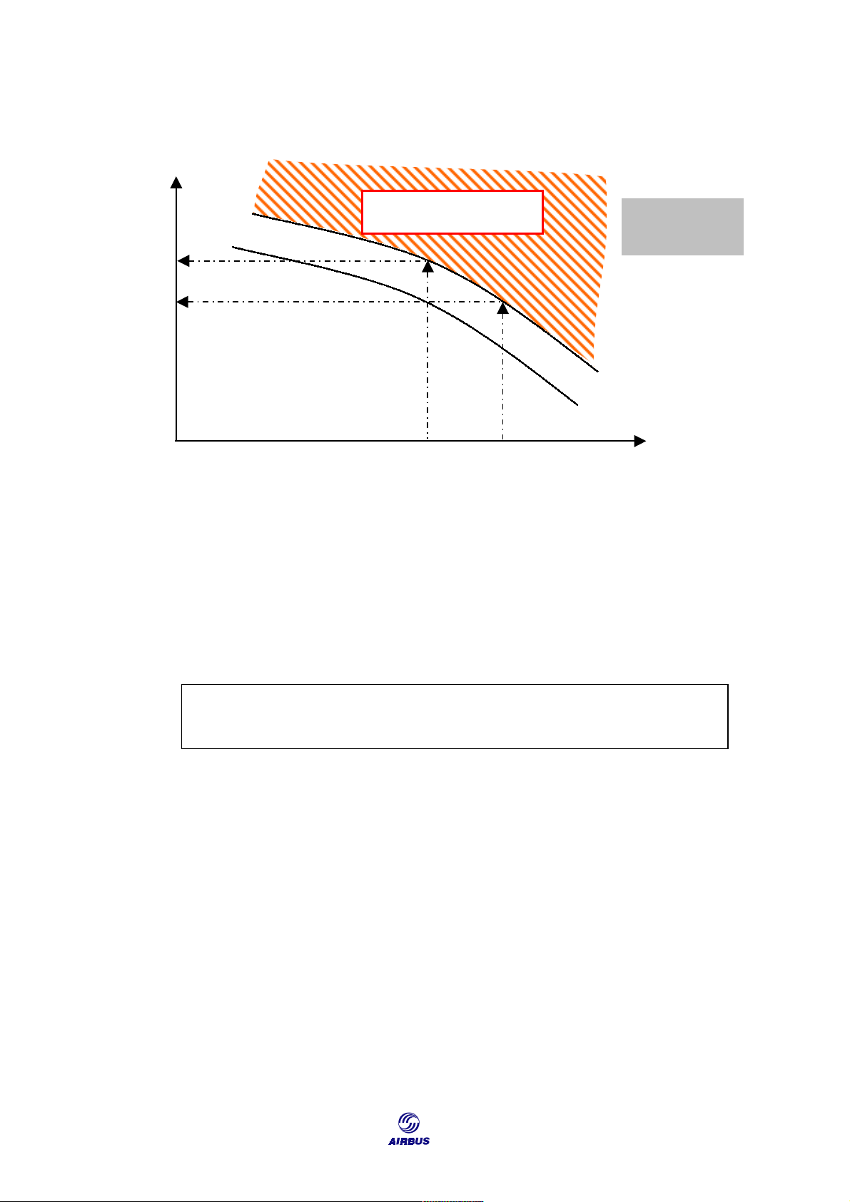
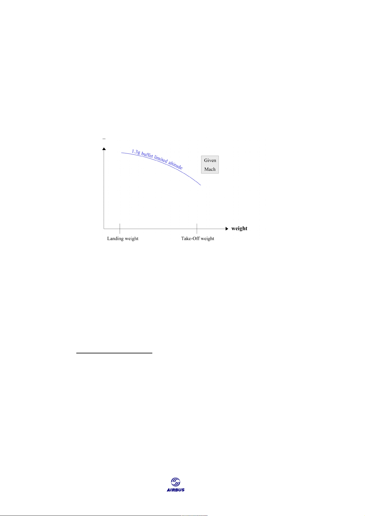
For a given Mach number, Figure F24 represents the 1.3g buffet limited
altitude versus weight. At a given Mach number, when weight Ì Ö the buffet limited altitude Ê. PA
Figure F24: 1.3g Buffet Limited Altitude
As a result, the maximum recommended altitude indicated by the FMGS,
depending on aircraft weight and temperature conditions, is the lowest of the:
• Maximum certified altitude, • Maximum cruise altitude,
• 1.3g buffet limited altitude,
• Climb ceiling (see the “Climb” chapter). 3.3.2.4. A320 example
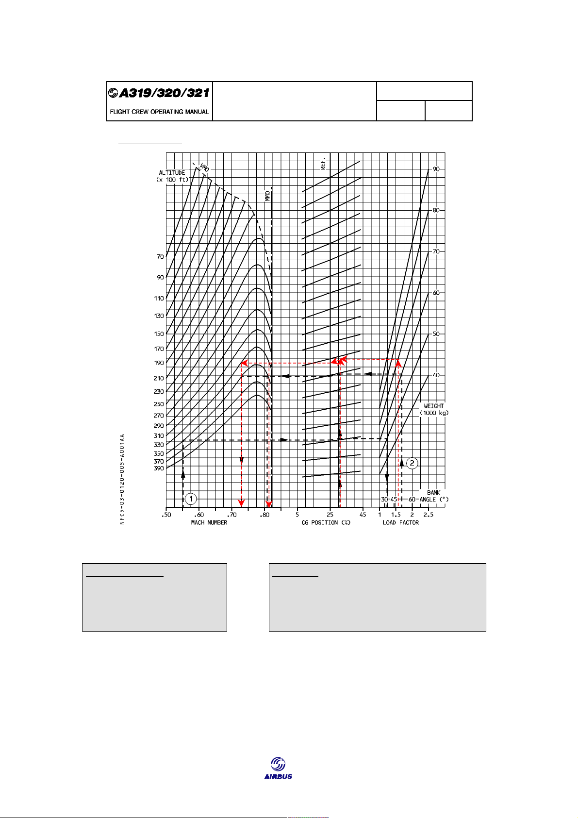
Figure F25 shows how buffet limitations are illustrated in an A320 FCOM. 145 CRUISE
Getting to Grips with Aircraft Performance OPERATING LIMITATIONS 3.01.20 P 5 GENERAL LIMITATIONS SEQ 001 REV 27 BUFFET ONSET R Figure F25: Buffet Onset Assumptions: Results: n = 1.3 Speed range: FL330 Mmin = M0.73 CG position: 31% Mmax = M0.82 Weight: 70 t
In practice, for a given weight, the load factor limitation (1.3g) is taken into account as follows:
• At a fixed FL, the cruise Mach number range is determined for n = 1.3g,
• At a fixed cruise Mach number, the maximum FL (buffet ceiling) is determined for n = 1.3g. 146
Getting to Grips with Aircraft Performance CRUISE
3.4. Cruise Optimization: Step Climb
Ideal cruise should coincide with optimum altitude. As a general rule, this
altitude is not constant, but increases as weight decreases during cruise. On the
other hand, ATC restrictions require level flight cruise. Aircraft must fly by segments
of constant altitude which must be as close as possible to the optimum altitude.
In accordance with the separation of aircraft between flight levels, the level
segments are established at ± 2,000 feet from the optimum altitude. In general, it is
observed that in such conditions: SR ≥ 99% SR max
As a result, the following profile is obtained for a step climb cruise (Figure F26). Given Mach number Maximum thrust limited altitude Step Climb 2,000 ft under FL 290 4,000 ft above FL 290 or 2,000 ft in RVSM area
Figure F26: A Step Climb Cruise Profile
Flight levels are selected in accordance with temperature conditions. Usually,
the first step is such that it starts at the first usable flight level, compatible with
maximum cruise altitude. This is the case with the ISA condition cruise example in Figure F26. 4. FCOM CRUISE TABLE
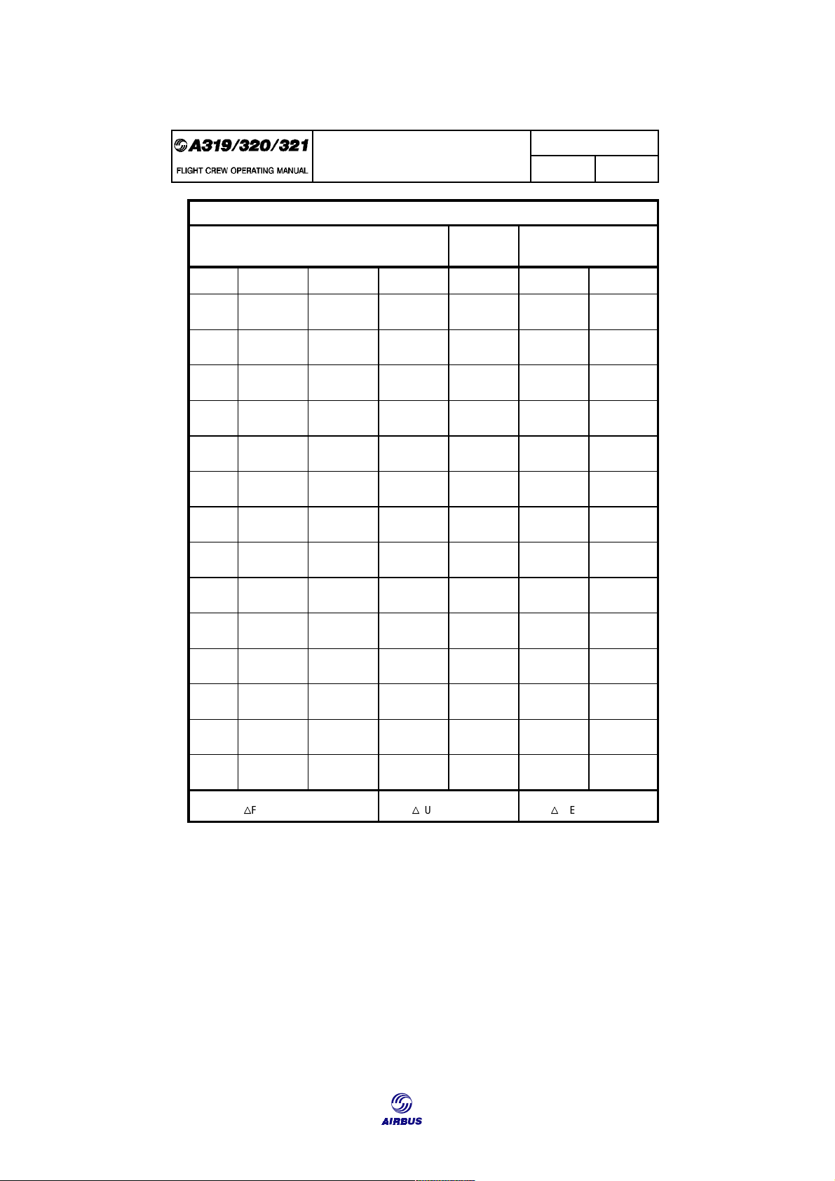
In the FCOM, cruise tables are established for several Mach numbers in
different ISA conditions with normal air conditioning and anti-icing off. Aircraft
performance levels are presented in Figure F27. 147 CRUISE
Getting to Grips with Aircraft Performance IN FLIGHT PERFORMANCE 3.05.15 P 9 CRUISE SEQ 110 REV 31 R CRUISE - M.78 MAX. CRUISE THRUST LIMITS ISA N1 (%) MACH NORMAL AIR CONDITIONING CG=33.0% KG/H/ENG IAS (KT) ANTI-ICING OFF NM/1000KG TAS (KT) WEIGHT FL290 FL310 FL330 FL350 FL370 FL390 (1000KG)
50 84.0 .780 84.0 .780 84.0 .780 84.1 .780 84.7 .780 85.9 .780 1276 302 1189 289 1112 277 1044 264 992 252 955 241 180.9 462 192.5 458 204.0 454 215.4 450 225.6 447 234.1 447
52 84.2 .780 84.2 .780 84.3 .780 84.5 .780 85.1 .780 86.3 .780 1288 302 1202 289 1127 277 1060 264 1011 252 977 241 179.2 462 190.3 458 201.4 454 212.0 450 221.3 447 229.0 447
54 84.4 .780 84.5 .780 84.6 .780 84.8 .780 85.5 .780 86.9 .780 1300 302 1216 289 1142 277 1079 264 1031 252 1003 241 177.5 462 188.1 458 198.6 454 208.4 450 217.0 447 223.1 447
56 84.7 .780 84.8 .780 84.9 .780 85.2 .780 85.9 .780 87.6 .780 1314 302 1231 289 1159 277 1097 264 1052 252 1036 241 175.7 462 185.9 458 195.7 454 204.8 450 212.6 447 216.0 447
58 84.9 .780 85.1 .780 85.2 .780 85.6 .780 86.4 .780 88.3 .780 1328 302 1246 289 1176 277 1117 264 1075 252 1070 241 173.9 462 183.6 458 192.8 454 201.3 450 208.1 447 209.0 447
60 85.2 .780 85.3 .780 85.6 .780 85.9 .780 86.9 .780 89.2 .780 1342 302 1262 289 1195 277 1137 264 1102 252 1110 241 172.0 462 181.3 458 189.8 454 197.6 450 203.0 447 201.5 447
62 85.5 .780 85.6 .780 85.9 .780 86.3 .780 87.6 .780 90.1 .780 1357 302 1279 289 1214 277 1158 264 1135 252 1153 241 170.1 462 178.8 458 186.8 454 194.1 450 197.1 447 194.0 447
64 85.7 .780 85.9 .780 86.2 .780 86.7 .780 88.2 .780 1373 302 1297 289 1234 277 1182 264 1170 252 168.2 462 176.4 458 183.8 454 190.2 450 191.2 447
66 86.0 .780 86.2 .780 86.6 .780 87.2 .780 89.0 .780 1389 302 1316 289 1254 277 1209 264 1209 252 166.2 462 173.9 458 180.9 454 186.0 450 185.0 447
68 86.2 .780 86.5 .780 86.9 .780 87.8 .780 89.8 .780 1406 302 1335 289 1275 277 1242 264 1252 252 164.2 462 171.4 458 177.9 454 181.0 450 178.7 447
70 86.5 .780 86.8 .780 87.3 .780 88.4 .780 90.8 .780 1424 302 1355 289 1299 277 1277 264 1298 252 162.1 462 168.9 458 174.6 454 176.1 450 172.3 447
72 86.8 .780 87.1 .780 87.7 .780 89.0 .780 1442 302 1375 289 1325 277 1314 264 160.0 462 166.4 458 171.2 454 171.1 450
74 87.1 .780 87.5 .780 88.2 .780 89.8 .780 1462 302 1397 289 1357 277 1356 264 157.9 462 163.9 458 167.1 454 165.7 450
76 87.4 .780 87.8 .780 88.8 .780 90.5 .780 1482 302 1419 289 1392 277 1400 264 155.8 462 161.3 458 162.9 454 160.5 450 LOW AIR CONDITIONING ENGINE ANTI ICE ON TOTAL ANTI ICE ON wFUEL = − 0.5 % wFUEL = + 2 % wFUEL = + 5 %
Figure F27: Cruise table example 148