Lecture 6: nonparametric techniques in density estimation môn Công nghệ thông tin| Trường Đại học Công nghệ Giao thông vận tải

CS434a/541a: Pattern Recognition Prof. Olga Veksler Lecture 6 Today
Introduction to nonparametric techniques
Basic Issues in Density Estimation Two Density Estimation Methods 1. Parzen Windows 2. Nearest Neighbors Non-Parametric Methods
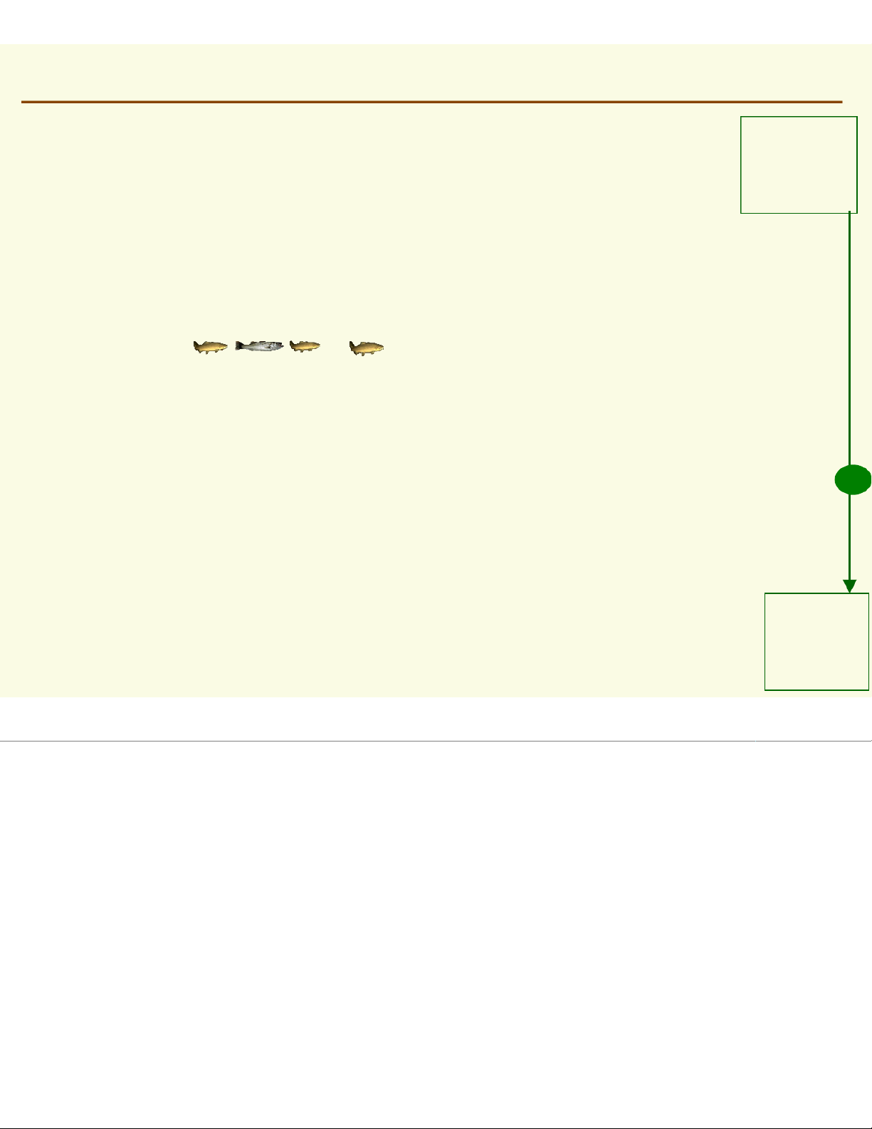
Neither probability distribution nor a lot is discriminant function is known known ”easier” Happens quite often All we have is labeled data salm s o a nlmon salmo b n ass
Estimate the probability distribution from the labeled data little is known “harder”
NonParametric Techniques: Introduction
In previous lectures we assumed that either
1. someone gives us the density p(x)
In pattern recognition applications this never happens 2. someone gives us p(x| θ) Does happen sometimes, but
we are likely to suspect whether the given p(x| θ) models the data well
Most parametric densities are unimodal (have a
single local maximum), whereas many practical
problems involve multi-modal densities
NonParametric Techniques: Introduction
Nonparametric procedures can be used with
arbitrary distributions and without any
assumption about the forms of the underlying densities
There are two types of nonparametric methods: Parzen windows Estimate likelihood p(x|cj) Nearest Neighbors
Bypass likelihood and go directly to posterior estimation P(cj| x)
NonParametric Techniques: Introduction
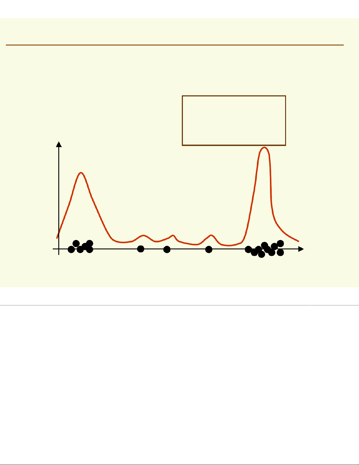
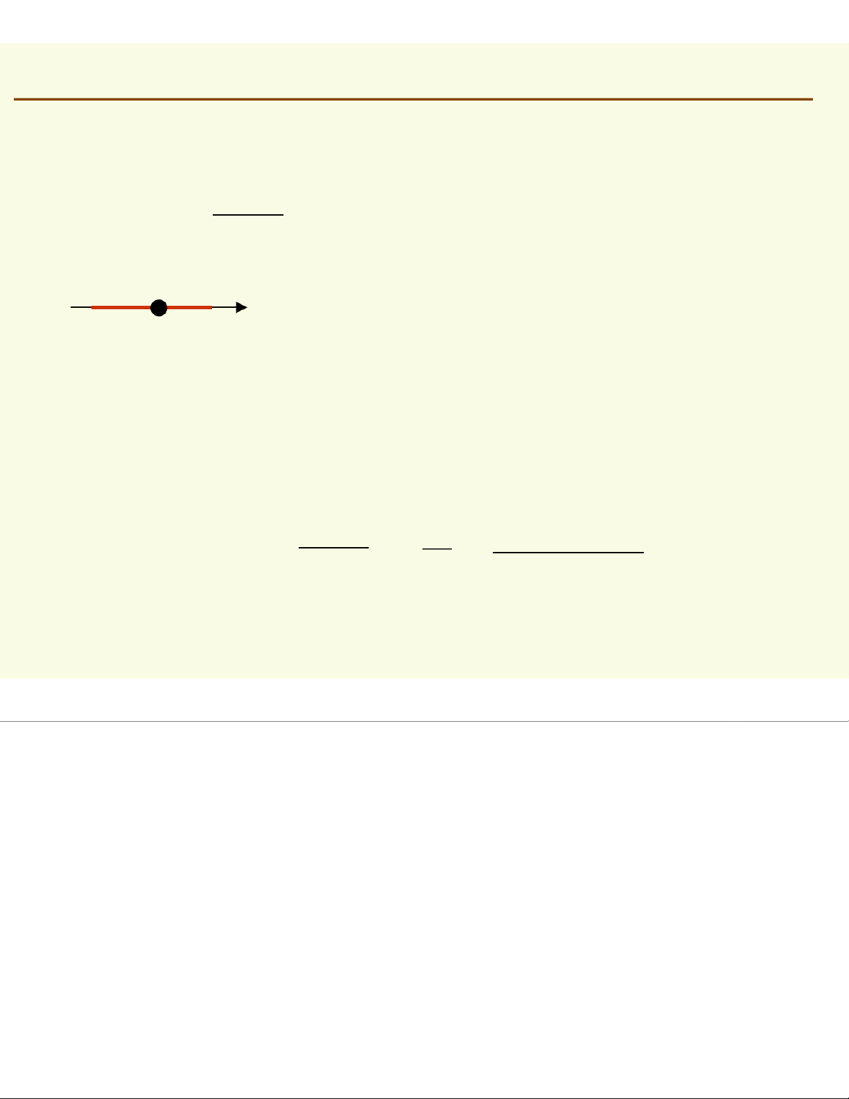
Nonparametric techniques attempt to estimate the
underlying density functions from the training data
Idea: the more data in a region, the larger is the density function Pr X [f x∈ ∈dx] ℜ = ( ) ℜ average of f(x) over p(x) salmon length x
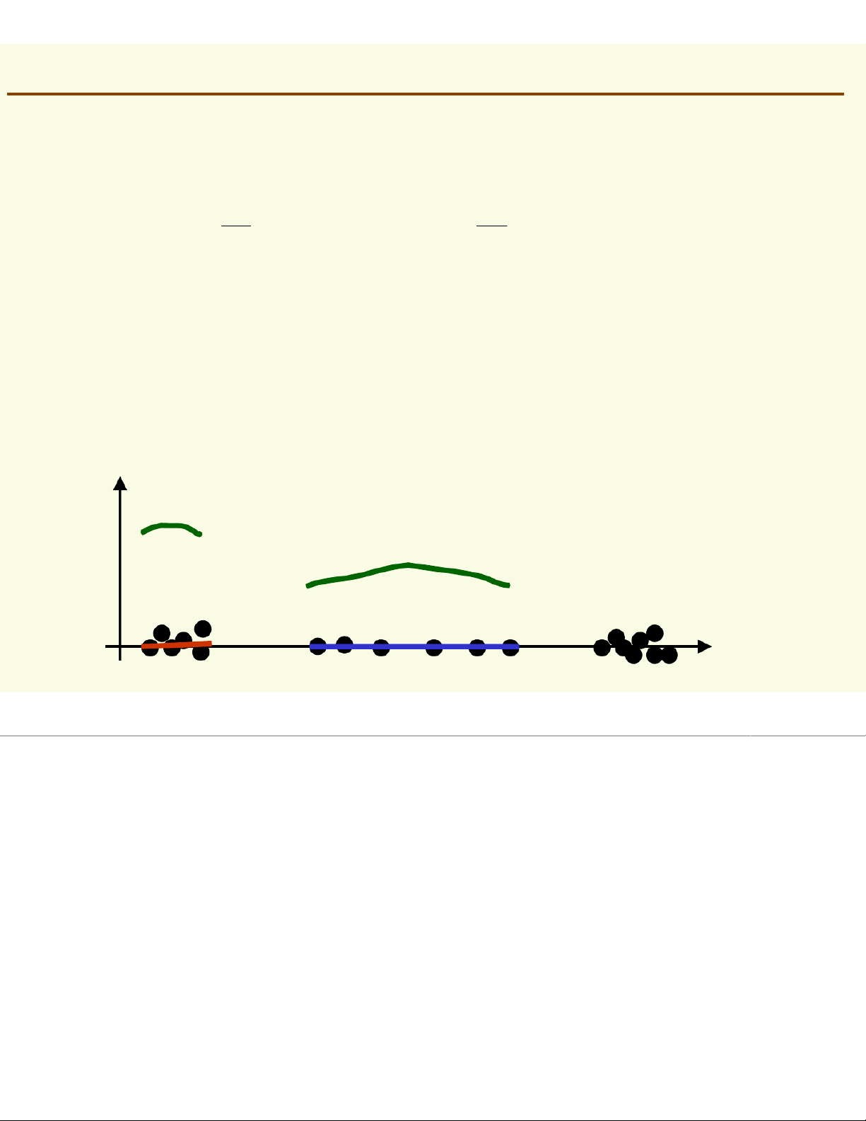
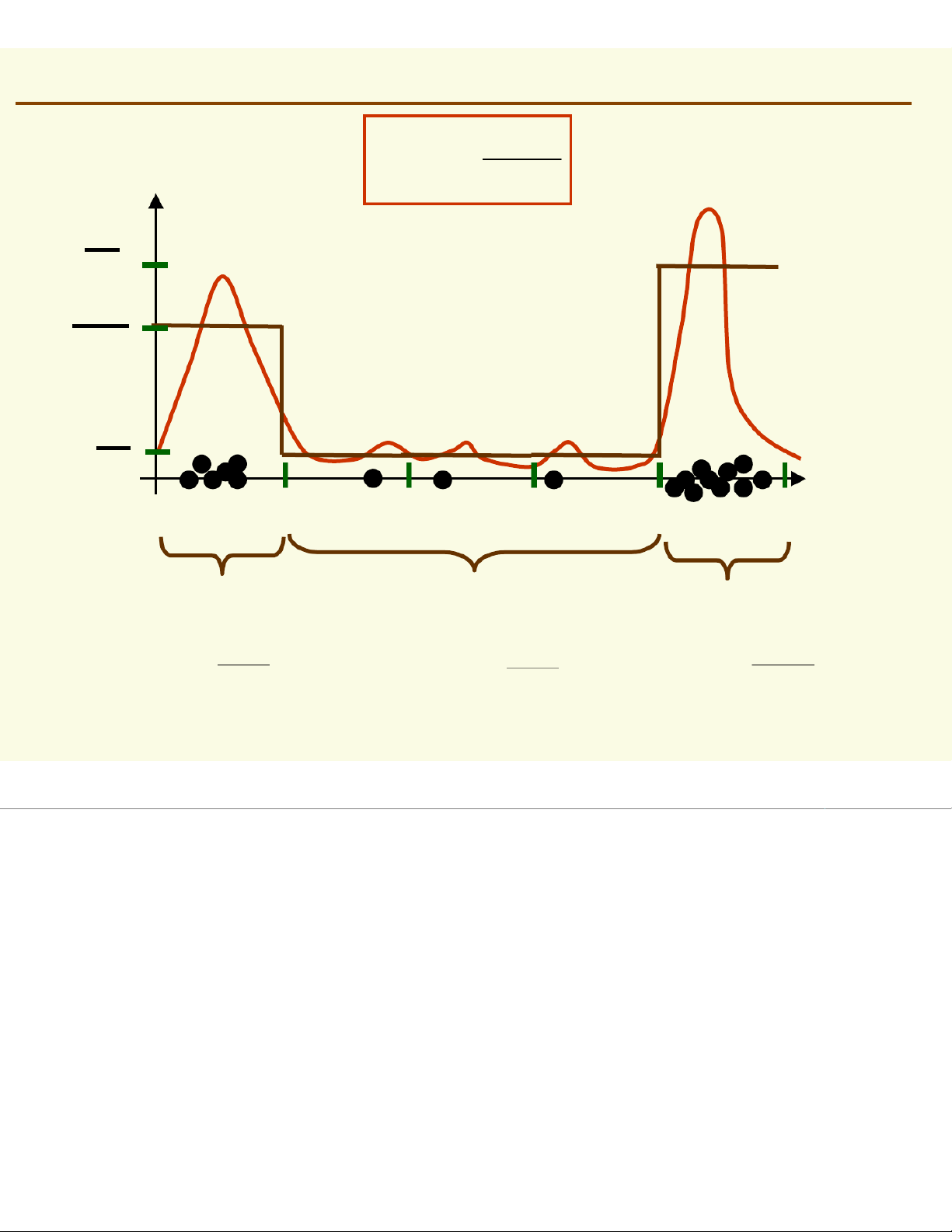
NonParametric Techniques: Introduction Pr X [f x∈dx] ℜ = ( ) ℜ How can we approximate P r [ X ∈ an ℜ d ] Pr [X ∈ ℜ ] 1 ? 2 6 6 and Pr [1 ] X ≈ ∈ ∈ ℜ ]≈ Pr [2 ] X ≈ ∈ ∈ ℜ ]≈ 20 20
Should the density curves above 1and 2be equally high? No, since is 1smaller than 2 f x dx f x [ dx P ∈ ∈ r 1 ℜ ]X= ( ) ≈ ( ) = [ ∈ ∈ 2 ℜ ] ℜ ℜ 1 2 ℜ
To get density, normalize by region size p(x) ℜ1 ℜ2 salmon length x
NonParametric Techniques: Introduction
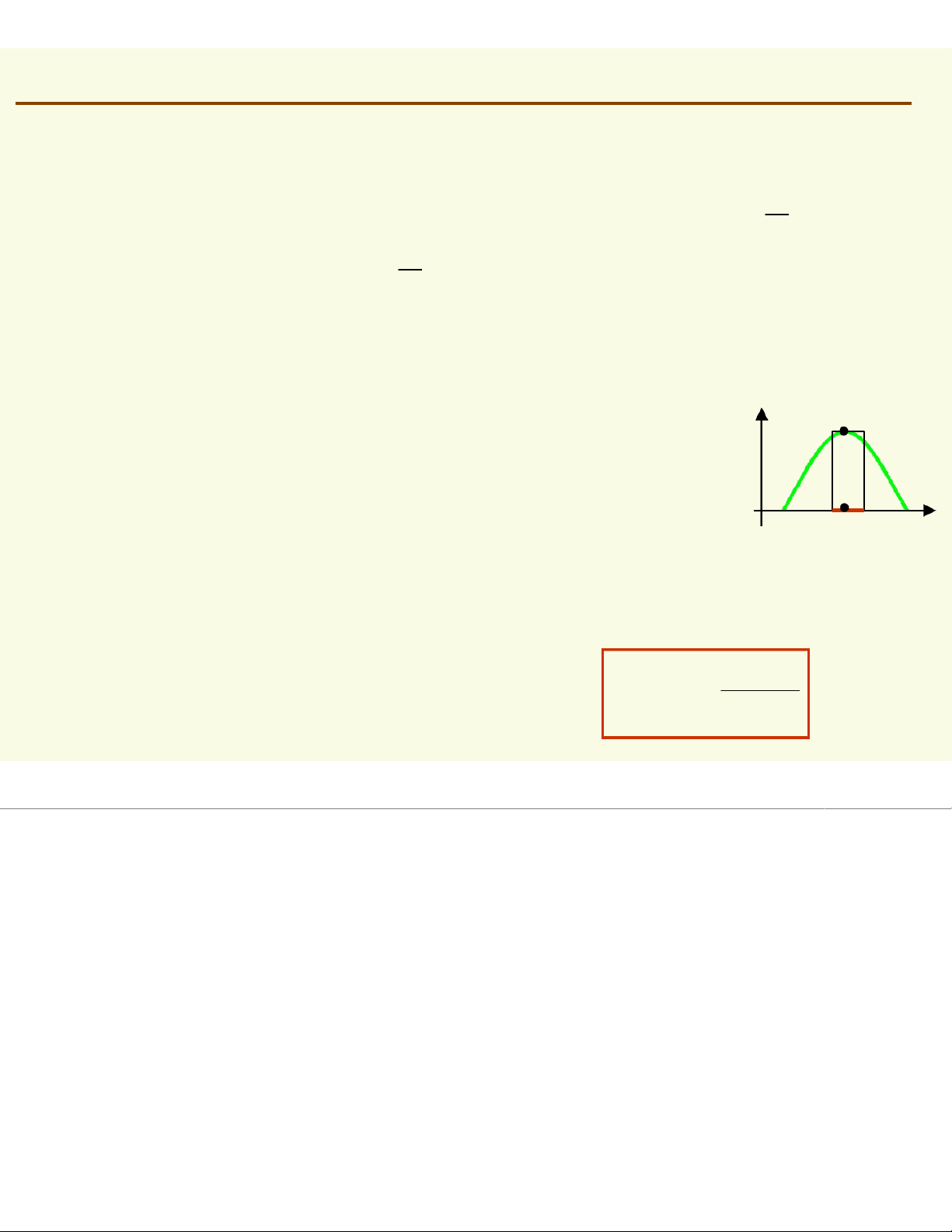
Assuming f(x) is basically flat inside # of samples in ℜ Pr X ≈ [f y∈ ∈dy] ℜ = ( ) ≈f (x )∗Volume ( ) ℜ total # of samples ℜ
Thus, density at a point xinside can be approximated f ( ) x (# of samples in ℜ 1 ≈Volume total # of samples ( )) ℜ
Now let’s derive this formula more formally Binomial Random Variable
Let us flip a coin ntimes (each one is called “trial”)
Probability of head ρ, probability of tail is 1- ρ
Binomial random variable Kcounts the number of heads in ntrials P (− ) K = k = ) ( n k = ρ ( ) 1 − ρ)n −k k n n! where k = k !(n)− k )! Mean is E (K )= nρ
Variance is Kvar (n )= ρ (1 − ρ )
Density Estimation: Basic Issues
From the definition of a density function, probability
ρ that a vector xwill fall in region is: p ( x' ) d ρ = x ' [ ∈ ] ℜ = ℜ
Suppose we have samples x1, x2,…, xn drawn from
the distribution p(x). The probability that kpoints fall
in is then given by binomial distribution: Pr [ ] K −= ] n k = − k ρ (1 − ρ)n k k Suppose that kpoints fall in , we can use MLE to
estimate the value of ρ . The likelihood function is p (− ) x ,..., x | ρρ ) n = k ρ (1 − ρ)n−k 1 nk
Density Estimation: Basic Issues p (− ) x ,..., x | ρρ ) n = k ρ (1 − ρ)n−k 1 nk k
This likelihood function is maximized at ρ ρ = n Thus the MLE is k ˆρn=
Assume that p(x)is continuous and that the region
is so small that p(x)is approximately constant in p(x) ( ' ) ' p ( x ) dx p ≅≅ ≅ x V ℜ x xis in and Vis the volume of Recall from the previous sli p de: x ( d' ) xρ =' ℜ Thus p(x)can be approximated: p (≈ ) x ) k / n ≈ V
Density Estimation: Basic Issues
This is exactly what we had before: p (≈ ) x ) k / n ≈≈x is inside some region V k = number of samples inside
n=total number of samples inside x V = volume of
Our estimate will always be the average of true density over p (x ' )dx ' ρˆ p (≈ ) x ) k / n ≈V =V ℜ ≈ V
Ideally, p(x) should be constant inside Density Estimation: Histogram p (≈ ) x ) k / n ≈ V p(l) 10 190 6 190 1 190 010 20 30 40 50 1 2 3 10/ 19 p(=) x 6 / 19 = p(=) x 3 / 19 = p(=) x = 10 30 10
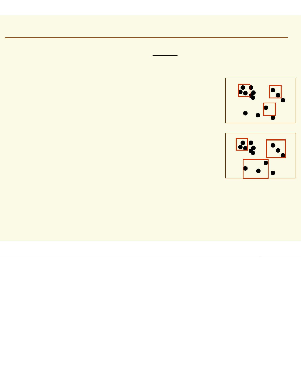
If regions i‘s do not overlap, we have a histogram Density Estimation: Accuracy
How accurate is density approximation p (≈ ) x ) k / n ≈ ?V
We have made two approximations k 1. ˆn ρ =
as n increases, this estimate becomes more accurate p (2. x ) dx p ≅≅ ≅ x V ℜas
grows smaller, the estimate becomes more accurate As we shrink we have to make sure
it contains samples, otherwise our estimated p( ) = 0 for all x xin
Thus in theory, if we have an unlimited number of
samples, to we get convergence as we
simultaneously increase the number of samples n, and shrink region , but not too much so that still contains a lot of samples Density Estimation: Accuracy p (≈ ) x ) k / n ≈ V
In practice, the number of samples is always fixed
Thus the only available option to increase the
accuracy is by decreasing the size of (Vgets smaller)
If Vis too small, p(x)=0 for most x, because most regions will have no samples
Thus have to find a compromise for V
not too small so that it has enough samples
but also not too large so that p(x) is
approximately constant inside V
Density Estimation: Two Approaches p (≈ ) x ) k / n ≈ V 1. Parzen Windows:
Choose a fixed value for volume V
and determine the corresponding k from the data 2. k-Nearest Neighbors Choose a fixed value for kand determine the corresponding volume Vfrom the data
Under appropriate conditions and as number
of samples goes to infinity, both methods can
be shown to converge to the true p(x) Parzen Windows
In Parzen-window approach to estimate densities we
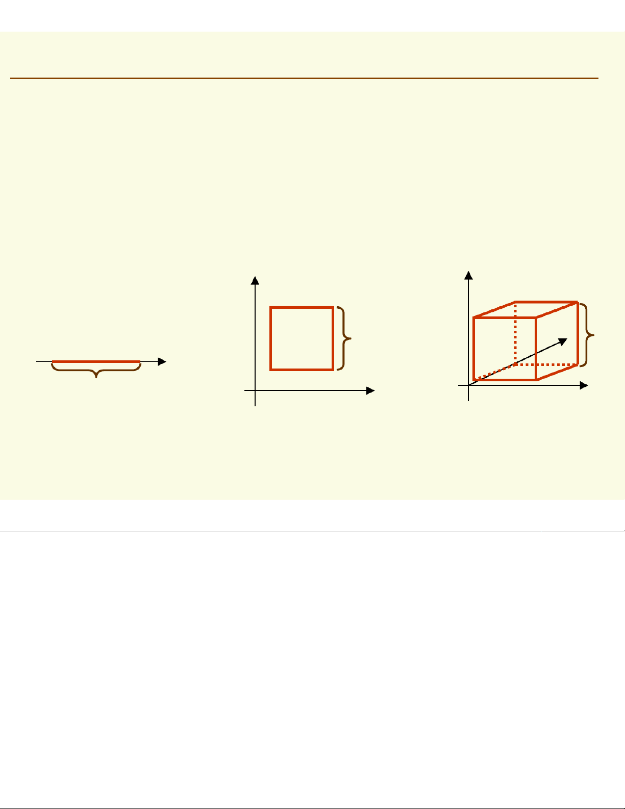
fix the size and shape of region Let us assume that the region is a d-dimensional
hypercube with side length h thus it’s volume is hd h h h 1 dimension 2 dimensions 3 dimensions Parzen Windows
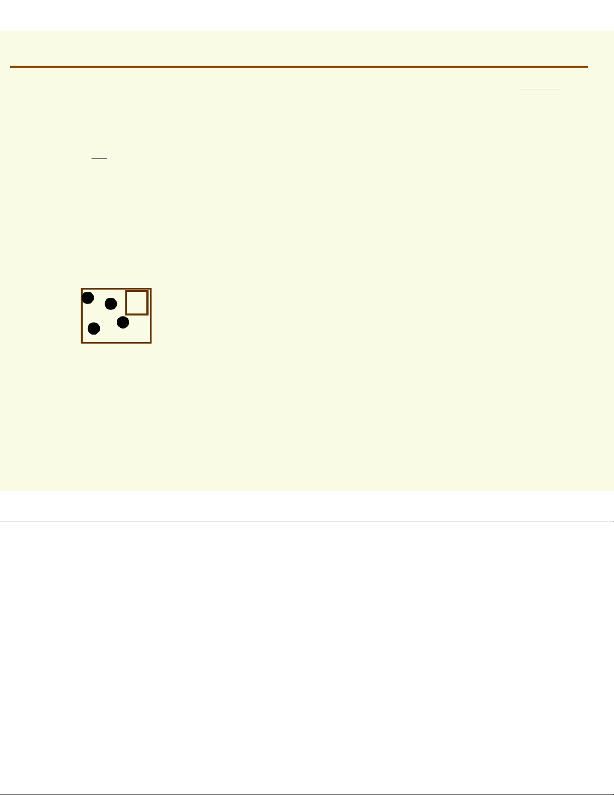
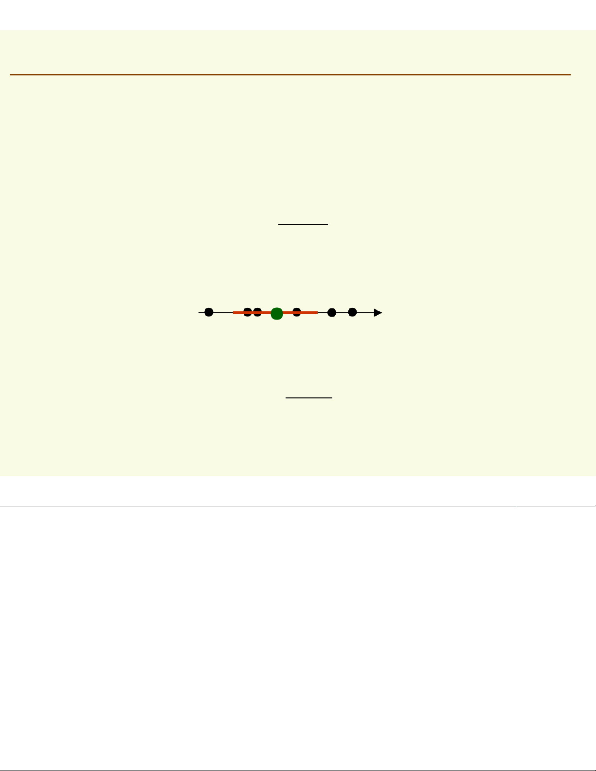
To estimate the density at point x, simply center the region
at x, count the number of samples in ,
and substitute everything in our formula p (≈ ) x ) k / n ≈ V x p (≈ ) x ) 3 / 6 ≈ 10 Parzen Windows
We wish to have an analytic expression for our approximate density
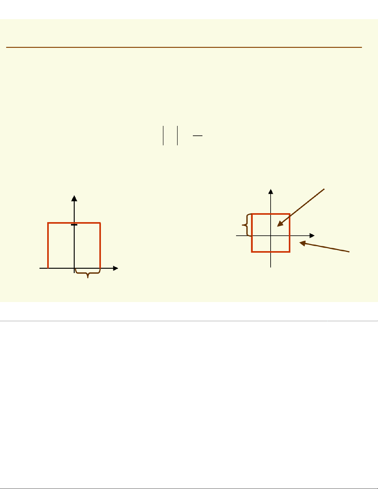
Let us define a window function = 1 1 u ≤ j =1,... ,d ϕ(u) = j2 0 otherwise ϕ is 1 inside 1 dimension u2 ϕ(u) 1 1/2 u1 u ϕ is 0 outside 1/2 2 dimensions Parzen Windows
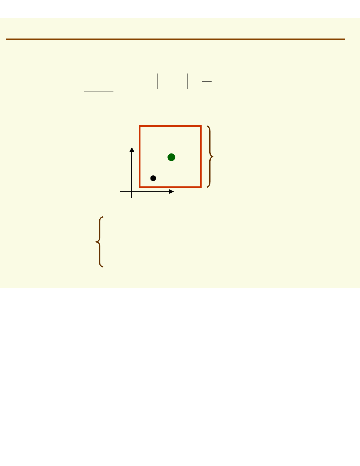
Recall we have samples x1, x2,…, xn . Then = h x - x 1 x - x ≤ j =1,... ,d ϕ(i i ) 2 = h 0 otherwise x h xi 1
if xiis inside the hypercube with x - x ϕ(i ) = width h and centered at x h 0 otherwise