


Preview text:
logistics Article
Use of Smart Glasses for Boosting Warehouse Efficiency:
Implications for Change Management
Markus Epe 1 , Muhammad Azmat 2,3,* , Dewan Md Zahurul Islam 4 and Rameez Khalid 5 1
Business School, University of Plymouth, Cookworthy Building, Plymouth PL4 8AA, UK; markusepe@outlook.de 2
Department of Engineering Systems and Supply Chain Management, Aston University, Birmingham B4 7ET, UK 3
Cluster of Supply Chain Management, Karachi School of Business and Leadership (KSBL), Karachi 74800, Pakistan 4
Newcastle Business School, Northumbria University, Newcastle upon Tyne NE1 8ST, UK; dewan.islam@northumbria.ac.uk 5
Management Department, School of Business Studies, Institute of Business Administration (IBA),
University Road, Karachi 75270, Pakistan; rameezkhalid@iba.edu.pk *
Correspondence: m.azmat@aston.ac.uk
Abstract: Background: Warehousing operations, crucial to logistics and supply chain management,
often seek innovative technologies to boost efficiency and reduce costs. For instance, AR devices
have shown the potential to significantly reduce operational costs by up to 20% in similar industries.
Therefore, this paper delves into the pivotal role of smart glasses in revolutionising warehouse
effectiveness and efficiency, recognising their transformative potential. However, challenges such
as employee resistance and health concerns highlight the need for a balanced trade-off between
operational effectiveness and human acceptance. Methods: This study uses scenario and regression
analyses to examine data from a German logistics service provider (LSP). Additionally, structured
interviews with employees from various LSPs provide valuable insights into human acceptance.
Results: The findings reveal that smart glasses convert dead time into value-added time, significantly
enhancing the efficiency of order picking processes. Despite the economic benefits, including higher
Citation: Epe, M.; Azmat, M.; Islam,
profits and competitive advantages, the lack of employee acceptance due to health concerns still needs
D.M.Z.; Khalid, R. Use of Smart
to be addressed. Conclusions: After weighing the financial advantages against health impairments, the Glasses for Boosting Warehouse
study recommends implementing smart glass technology in picking processes, given the current state
Efficiency: Implications for Change
of technical development. This study’s practical implications include guiding LSPs in technology
Management. Logistics 2024, 8, 106.
adoption strategies, while theoretically, it adds to the body of knowledge on the human-technology https://doi.org/10.3390/ interface in logistics. logistics8040106
Academic Editors: Mladen Krsti´c,
Keywords: order picking; smart glasses; smart warehouse; digitalisation; warehouse operations;
Željko Stevi´c and Snežana Tadi´c
logistics performance; warehouse performance; smart logistics; innovation Received: 23 July 2024 Revised: 15 September 2024 Accepted: 30 September 2024 1. Introduction Published: 17 October 2024
In today’s global supply chains, the demand for speed and agility in logistical processes
is imperative, particularly within warehouse operations, where efficiency is a crucial
determinant of success [1]. Order picking is a part of the warehousing logistical processes
Copyright: © 2024 by the authors.
in a company that has a vital impact on performance in terms of efficiency, quality, cost,
Licensee MDPI, Basel, Switzerland.
and time [2]. Order picking as an essential part of the material flow is a value-intensive
This article is an open access article
activity with great potential for optimisation [3]. Recognising this potential for optimisation,
distributed under the terms and
pursuing efficiency in this process becomes crucial to reduce operational costs and enhance
conditions of the Creative Commons
picking speed [4]. To do so, new methods, products, and services are required to meet the
Attribution (CC BY) license (https://
demands of highly dynamic logistics markets and the increasing complexity of logistics
creativecommons.org/licenses/by/
networks. Flexibility, adaptability, and proactivity are becoming increasingly important 4.0/).
Logistics 2024, 8, 106. https://doi.org/10.3390/logistics8040106
https://www.mdpi.com/journal/logistics Logistics 2024, 8, 106 2 of 25
and can be achieved by incorporating new technologies [5]. While problem-orientated
approaches lead to incremental improvements, technology-orientated approaches can bring
more significant changes [6]. Employees still manually carry out many logistics processes
according to the receipt-based pick-by-paper or the receipt-less variant pick-by-scan [7].
Securing competitive advantages by improving order picking performance is crucial
for a warehouse operation’s competitive positioning. Innovative technologies such as
augmented reality (AR) are proving particularly promising for logistics in warehousing.
AR can reduce warehouse operations costs while significantly increasing efficiency and productivity [8].
Employees must perform information-intensive activities within order picking while
keeping their hands free to carry out picking activities. In the form of smart glasses, AR
can display context-sensitive information in the user’s field of vision and guide them
through work steps [9]. Smart glasses thus extend current picking scenarios through so-
called pick-by-vision systems [10]. As a result, the employees engaged in transport and
logistics operations, equipped with smart glasses, are provided with real-time operational
information, such as delivery orders and picking status, without interrupting the actual
work process to improve performance [9,11]. The glasses offer a novel aspect of current
picking situations, providing employees with instant operational information without
unduly interrupting their work process.
In an experiment, DHL tested two commercial smart glasses, Google Glass and Vuzix®
M100, at a warehouse and discovered a 25% boost in efficiency [12]. Similarly, Boeing
investigated using Google Glass to help in wire bundle assembly; they observed a 30%
boost in productivity and a favourable response from employees [13]. In another case study,
a head-worn display (HWD) was implemented in two warehouses in Belgium, where one
was successful while the other was not. The prime reason was the employees’ involvement
in improving the device’s functionality and usage conditions [14]. Another study reported
four cases of implementing AR-enabled vision-picking at DHL, Samsung, Coca-Cola, and
Intel. At DHL, productivity and speed increased by 15% and 25%, respectively, while
at Samsung, productivity increased by 12–22%. Similarly, at Coca-Cola, performance
increased by 6–8%, while at Intel, speed increased by 29% [15].
Although the literature focusses on the potential of smart glasses in warehousing,
scientific case studies still need to be developed, leading to a gap in understanding their
efficiency and effectiveness [16–18]. Despite its maturity, the use of AR systems in ware-
housing, especially in the order picking process, is still an active area of research [19]. The
authors of [20] emphasised that there is a need to share selected use cases to resolve any
uncertainties in logistics regarding the use of AR-enabled smart glasses. The literature
further stressed assessing the impact of smart glasses via well-documented case studies
experimenting with various digital technologies and software and rigorous comparisons
with existing solutions [20,21]. Comfort and cleanliness in reusing these glasses across
multiple shifts require further testing, posing significant barriers to user acceptance and adoption [22].
The gap that this study plans to fill is to determine the productivity benefits of smart
glasses over traditional picking methods along with their human acceptance. To fill this
identified gap, a research question is posed: Can smart glasses be more effective, efficient, and
acceptable than conventional order picking methods for logistics processes? In answering this
question, the paper aims to investigate the effects of smart glasses in terms of effectiveness
and efficiency increase and acceptance compared to conventional picking methods in
a case study in cooperation with a German 3PL service provider, as well as to evaluate the
employee acceptance of smart glasses.
The study seeks to understand smart glasses’ potential for transformative capabilities
by applying scenario analysis, regression analyses, and structured interviews of employees.
The research question is further explained by creating the research objectives, which will
be presented in the next section. Logistics 2024, 8, 106 3 of 25 2. Literature Review
Picking is one of the core activities of a warehousing operation. As per [23], it is the
most time-consuming and error-prone activity among all the warehousing tasks. Today,
there are multiple ways in which orders are picked in warehouses, namely: pick-by-paper,
pick-by-vision, pick-by-light, pick-by-voice, pick-by-gesture, cart-mounted display, and
pick-by-scan [21]. Most warehouses still use paper-based picking approaches. However,
any paper-based approach could be faster and more accurate. In addition, picking is often
performed by temporary workers, who usually require costly training to ensure efficient
and error-free picking [23]. In this section, we will first discuss the key performance indica-
tors (KPIs) involved in assessing the performance of a picking operation in a warehouse.
Subsequently, the role of human touch and smart glasses in pick-by-vision will be discussed.
This section will conclude with a discussion of the benefits of AR-enabled picking and the
research objectives of this study. 2.1. KPIs in Picking Operation
Efficiency is the improved ratio of (minimum) input to (maximum) output. Logistics’
primary and most important purpose is to connect supply and demand in a demand-
orientated and cost-efficient way [24]. To improve competitiveness, the efficiency of logistics
facilities (quantity, speed, and quality with the same resource input) must be increased [24].
To improve performance, reducing the amount of redundant resources is necessary [25].
The key performance indicators (KPI) are throughput times, picking performance, and the
associated error rates [26,27].
Throughput Time: Picking time can be defined as the throughput time of the picking
process [28,29]. The throughput time of an order is defined as the sum of the processing,
transport, and waiting times at all production stages [30], therefore, the sum of dead
times, picking times, and travel times across all items [31,32]. An order picking system’s
KPI “picking performance” is relevant to reflect its efficiency [33]. Usually, the picking
performance refers to the number of items regardless of the removal quantity per item [29].
The performance is always related to a time unit, which is always one hour. Following
Equation (1) is formulated to calculate the order picking performance. Pos Order picking per f ormance = (1) h
Picking Performance: Other variables influencing performance are the availability and
utilisation of order pickers. There are empirical values for the availability of human order
pickers [33] based on the working conditions and the load. In performance comparisons of
picking techniques, the number of positions “Pos” is kept constant so that the picking time
is multiplied by the same factor each time. The performance is thus directly proportional
to the picking time [30]. Depending on the throughput time and the number of positions,
the order picking performance can be determined with Equation (2) below, which is
increasingly applied in further processes. Pos Number o f positions Order picking per f ormance = ∗ 60 min/h (2) h throughout time [min]
Error Rate: One of the most critical factors in picking is avoiding or reducing errors.
Pick errors can directly impact customer relationships and satisfaction, as picking errors
are often noticed after delivery. Errors, therefore, result in a negative customer experience,
which can affect the customer-supplier relationship and result in financial damage [34].
According to [23,33], one error per 1000 items (0.1%) is desirable. The goal of zero error Logistics 2024, 8, 106 4 of 25
picking is currently not achievable due to human error susceptibility in a non-autonomous
picking system. The following Equation (3) is used to calculate the error rate: Number o f errored positions Error rate [%] = ∗ 100% (3) Number o f positions
Out of the four methods (pick-by-scan, pick-by-voice, pick-by-light, and pick-by-
vision), only one picking method is below the desirable error rate of 0.1% (see Table 1),
and that is the pick-by-vision method having an average error rate of 0.08%. Although the
error rate in order picking today is meagre even with a pick-by-paper approach—experts
estimate the rate at 0.35% to 0.45%—every error must be avoided as it usually results in
high follow-up costs [35]. Table 1 establishes pick-by-vision as a candidate to be explored
further for wider application due to its potential to reduce error. In a lab test, an optimal
set of parameters were extracted for the best performance: the battery is to be positioned
on the side of the weight, the storage level of the racks should be high, discrete order mode
of picking should be used, a scanner should be used as the confirmation equipment, and
there should be a lower number of lines per order.
Table 1. Overview of Error Rates, compiled from various sources [1,29,36–39]. Method Error Rate Source Average Error Rate 0.36% (Günthner, et al., 2009) Pick-by-Scan 0.46% (ten Hompel and Schmidt, 2010) 0.39% 0.36% (Lolling, 2003) 0.25% (Reif, 2009) Pick-by-Voice 0.08% (ten Hompel and Schmidt, 2010) 0.14% 0.10% (Lolling, 2003) 0.25% (Reif, 2009) Pick-by-Light 0.08% (ten Hompel and Schmidt, 2010) 0.24% 0.40% (Lolling, 2003) 0.0075% (Guo, et al., 2014) Pick-by-Vision 0.125% (Göpfert and Kersting, 2017) 0.08% 0.12% (Günthner, et al., 2009) 2.2. Human Touch in Picking
Human flexibility in order picking is almost impossible to replace, despite many
automation concepts. Regardless of increasing requirements such as variable article ranges,
decreasing order sizes, and increased flexibility, rationalisation potentials can be tapped
if the order picker is optimally supported in their core task, considering both ergonomic
and informational aspects, and is relieved of time-consuming and distracting secondary
activities [29]. AR can improve information visualisation if employees in picking systems
are equipped with data glasses [40]. Ref. [14] identified a need to document cases where
companies have successfully maintained and extended employee interest and participation
while implementing smart glasses in picking operations.
2.3. Smart Glasses for Pick-by-Vision
‘Smart glasses’ refers to peripheral devices with integrated small computers worn
on or at the head. Things, plants, animals, people, situations, and processes are regis-
tered, analysed, and enriched with virtual information [41]. Mobile devices attached to
the user’s body are called wearables [42]. A wearer of smart glasses, or more broadly,
an augmented reality head-worn display HWD (AR HWD), can access various informa-
tional types, such as text, graphics, and video. Information can be overlayed onto the
real world (augmented vision) or perceptually placed next to real-world objects of interest
(conformal augmented reality) so that users do not have to look down to access it, unlike
when they access manuals, hand-held devices, or other reference materials [12]. Typically,
the aim is to support real-world action by offering data, assessments, and directions [43,44]. Logistics 2024, 8, 106 5 of 25
AR-enabled smart glasses can merge the actual world with virtual data in the user’s field of
vision. These AR devices must be distinguished from their virtual reality (VR) equivalents,
which have an opaque screen. They do not support the overlay of virtual and physical
reality but rather conceal the user’s perspective within the device and protect them from
any exterior visual input [45].
AR offers the possibility of actively supporting work processes in logistics, such as the
warehouse picking process, thereby increasing employee efficiency, effectiveness, and satisfac-
tion [8,46]. Various cases and experiments have been reported in the literature [12–15,22,47].
The integrated scanning technology, usually in the form of a camera on the frame of the
glasses, meets the demand for integrating digitisation measures, such as optimising ware-
house management systems [29]. Different smart glasses and scanners are reported in
the literature for pick-by-vision, to name a few: Google Glass, Vuzix® M100 and M300XL,
RealWear HMT-1, Samsung Gear S2, and Intel Recon Jet Pro.
Picking is a skill-, rule-, and information-intensive activity, so this technical support for
using AR and smart glasses in the pick-by-vision process is one of the most critical success
factors [36]. Using a tracking system to recognise the position and direction of gaze, static
data such as text information can be displayed and data that is dynamically positioned
in space [29]. These 3D spatial geometries attractively highlight the picking or storage
location or show the optimal path throughout the warehouse [29]. This always gives the
user direct access to information and eliminates the need for disruptive activities to retrieve
information that interrupts the work process. Furthermore, when using smart glasses, the
user has both hands free through voice-based control [8,23]. Increased picking performance
in the work process is expected through the expansion of the natural environment. This is
because of the process guidance along the picking process, which promises cognitive relief
for the smart glasses user [48].
2.4. Benefits of Paperless Picking
The strict visual guidance of order pickers lets them complete their daily picking tasks
in a warehouse environment faster and more error-free than they would be able to do
without the support of data glasses [49]. According to [49], smart glasses make it possible to
use an ergonomic product that can be worn by the order picker and the cognitive superiority
of humans to design logistical processes efficiently. Previous studies in paperless picking
suggest that data glasses have great potential as a user-friendly and task-supporting tool
with good information display and design quality [50]. It was also found that the error
rate is significantly lower when using pick-by-vision compared to voice-controlled picking
support. This is due to the technically determined low error tolerance of data glasses [51].
Refs. [52,53] suggest that paperless picking methods have tremendous advantages.
Pick-by-vision leads to reduced search times, clean documentation, increased performance,
and reduced errors in the picking process. The use of smart glasses offers the opportunity to
actively support work processes in logistics, such as the picking process in the warehouse,
thereby increasing efficiency, effectiveness, and employee satisfaction [8,46]. Especially in
throughput time, pick-by-vision can achieve a competitive advantage. The authors of [20]
have defined the potential of AR smart glasses in logistics and supply chain management
around four facets: visualisation, interaction, user convenience, and navigation.
A faster process goes hand in hand with higher productivity, increasing profitability.
The faster an order is picked up, the cheaper the product delivery. Other goals are route
optimisation, increased picking performance based on short throughput times, and process
reliability in the form of little to no error susceptibility. The processing of the order volume
should require as little effort as possible and must accordingly be designed as efficiently as
possible [7,52]. In this context, the employee’s movement time plays a significant role at
50%, and the search time is 20% within the picking process (Figure 1) [54]. Logistics 2024 Logistics , 20248 , , 8106 , x FOR PEER REVIEW 6 of 6 of 25 27 % of Order-Picker's Time Other Setup Pick Search Travel 0% 10% 20% 30% 40% 50% 60%
Figure 1. Order picking time overview [48].
Figure 1. Order picking time overview [48]. 2.5. 2.5. Derivation
Derivation of the Resear of the Resear ch Objec ch tives Objectives Order pick Order ing take picking s sev takes eral several items fro items fr m om the w the areh war ouse to serv ehouse to e serve and and fulfi fulfill several several independent independent customer ord customer or ers ders accord accor ing to cu ding to stomer requirements. customer requirements. The aim is The aim is to to make make this this process process as as pr practical actica (e.g., l (e.g., higher higher speed of speed of p picking) ic and king ef ) and ficient effi (e.g., cient ( r e educed .g., reduced operational operat cost) ion as al cost possible. ) as pos This sib meansle. Thi that s me the ans t basic hat the operational basic costs operat shouldional c be r osts educed, should be but at the reduced, b same time, ut a the t the or sa der me time, the order picking speed pi should cki be ng spe incr ed eased sho [4]. uld be increas Minimising ed time[4]. M for inimis the ing picking time f pr o ocess r the p is icking process
necessary for any is necessary f picking o system r [ any 48, pic 55]. king system By extending [48,55]. B the y natural extending envir the onment, natur incr al envir eased onment, incr picking eased pic performance in kin the g per work formanc process e in is the wor
expected. k process is expected. Pick-by-vision can be Pick-by-v used ef ision can be ficiently, use primarily d e for fficiently, primar inexperienced ily for inexperience employees or high d employ temporary ees or high worker rates te in m a porary w company o . rker r The r ates in eason a com for this pany is, . The reason among other for t things, his i the s, among ot guidance her t along h theings, the picking gui pr dance ocess, along t which h pr e pickin omises g process cognitive ,r which promis elief for the es cognit smart ive re glasses lief fo user [48 r t ]. he sm These art glasse should s be user pr [48] ovided. Th to ese the shou e ld be mployee provided intuitively to th and e emplo er yee int gonomically uitive while ly and er aiming gonomic for an ef ally wh fective ile and aim ef ing for ficient an eff picking ectiv pr e and ocess, i effi .e., cient picking maximising process, i.e., performance maximising perf while ormanc minimising the e while potential minimising
for errors [ the potential for errors [46]. The st
46]. The strict visual guidance of or rict der visual pickers guidanc lets e them of order p complete ickers their lets daily them compl picking e tasks te thei in a r dai war ly pi ehouse cking ta envir sks i onment n a w faster areh and ouse env more err iron or-fr m ee ent faster than they and more would be error-f able to ree than they woul do without the d be a support b ofle to do data without the support of glasses [49]. data glasses [49]. The fo The llowing following re r sear esear ch obj ch ective i objective s is derived derived to m to ake the theory ta make the theory ngible a tangible nd crea and cr te a eate a possibility of verification. possibility of verification.
RO1: To assess the impact of smart glasses in increasing the effectiveness and efficiency of the
RO1: To assess the impact of smart glasses in increasing the effectiveness and efficiency of the
picking processes compared to conventional picking methods.
picking processes compared to conventional picking methods.
It emphasises exploring the improvement in logistics processes with the use of smart
It emphasises exploring the improvement in logistics processes with the use of smart
glasses and eventually offers the possibility of a competitive advantage.
glasses and eventually offers the possibility of a competitive advantage.
Humans will continue to play a crucial role in production and logistics operations due
Humans will continue to play a crucial role in production and logistics operations
to their adaptability and sensorimotor abilities in an increasingly digitalised world. Thus,
due to their adaptability and sensorimotor abilities in an increasingly digitalised world.
ergonomics, flexibility, and occupational safety should be improved [56]. The goal is to
Thus, ergonomics, flexibility, and occupational safety should be improved [56]. The goal
design logistics operations processes so people and machines can operate, interact, and
is to design logistics operations processes so people and machines can operate, interact, integrate easily [57]. and integrate easily [57].
Several strategies aim to increase user friendliness and acceptance by deliberately
Several strategies aim to increase user friendliness and acceptance by deliberately
minimising the number of necessary contacts between humans and the system. This
minimising the number of necessary contacts between humans and the system. This
allows the user to concentrate more on their task, increasing productivity and reducing
allows the user to concentrate more on their task, increasing productivity and reducing
the susceptibility to workplace errors. Intelligent devices are designed to be as invisible as
the susceptibility to workplace errors. Intelligent devices are designed to be as invisible as
possible to the user and to support him in his activity by providing him with the appropriate
possible to the user and to support him in his activity by providing him with the contextual information [57].
appropriate contextual information [57].
For pick-by-vision and the associated process optimisations to result in actual human-
For pick-by-vision and the associated process optimisations to result in actual
added value, it is crucial to consider factors influencing the acceptance and usability of the
human-added value, it is crucial to consider factors influencing the acceptance and information system [23,58,59].
usability of the information system [23,58,59].
To increase user acceptance, it is essential to consider both the physical and psycho-
To increase user acceptance, it is essential to consider both the physical and
logical strain on the employee [57]. Ergonomics and mental stress are the most crucial psycholog requir ica ements l strain for on the employ accepting smart ee [57]. devices [58].Ergonomics and Employees must ment be al stress are aware of the the most advantages
crucial requirements for accepting smart devices [58]. Employees must be aware of the Logistics 2024, 8, 106 7 of 25
of wearable technology and incorporate it into their everyday work activities. Wearables
should offer quantifiable value, for instance, regarding mobility or weight. Ideally, they
should not be noticeable to the employee in the work process but should integrate natu-
rally [60]. However, ergonomics is not limited to the wearability of smart glasses but also
to the ergonomics of the user interface. It is possible that extended use of smart glasses in
workplaces can cause visual fatigue and impair attention [61]. Although AR helps lessen
head and neck motions while operating, workers may become distracted or confused by the information [62].
In addition to ergonomics, an essential aspect of acceptance is privacy and the associ-
ated protection of that privacy [59]. The challenge is that indoor localisation and task and
error tracking are critical to the performance of such a system [63]. This exposes users to
increased surveillance by supervisors [59].
The following research objective is derived to make the theory tangible and to create
a possibility of assessing acceptability based on various criteria:
RO2: To assess the employees’ acceptance level of using smart glasses in the picking process without concerns. 3. Methodology
As mentioned in previous sections, this study has one research question and two
objectives. A mixed-method study was conducted to achieve the objectives, and the
following steps were implemented. 3.1. Research Objective 1 a.
The following methods were performed to assess the increase in efficiency of smart glasses in picking operations. i.
Two test series (one was in a test environment while the other was in live
business operation) were conducted in the year 2022 in the warehousing
facilities of the case company, i.e., the German 3PL logistics service provider
(LSP). The data on the same picking process with and without using smart
glasses was collected for comparison. The process flow within the two tests
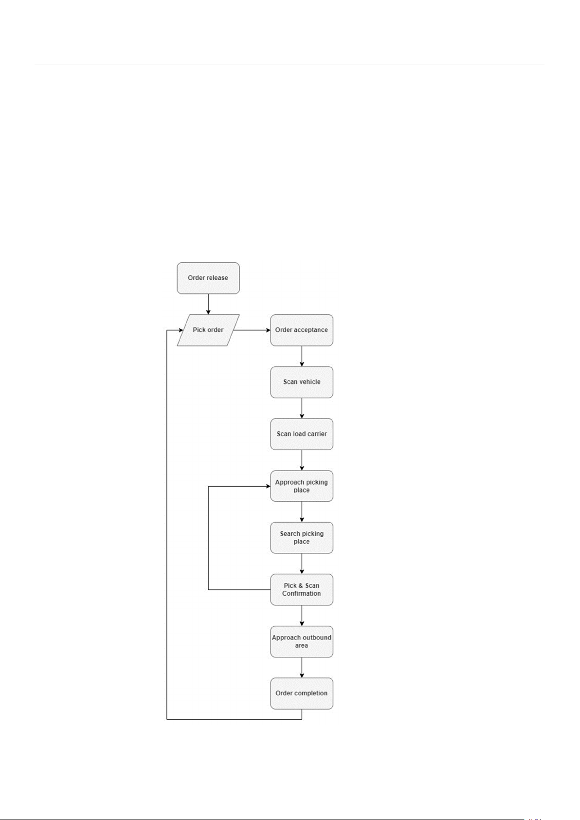
was defined in advance (Appendix A). During the data collection phase, the
employee is accompanied over one week to collect all the data. The same
selector performed the picking operation in both test series to reduce external
and human influences, such as picking and moving speeds. ii.
Based on the collected data, a regression analysis was conducted to deter-
mine the relationship strength between the dependent variable (throughput
time) and the independent variables (setup time, search time, and pick time).
Waiting time and travel time were kept constant. iii.
Ten scenarios were created using the collected data and historical data on
order picking from the case company for 2021. These scenarios were thor-
oughly evaluated to generalise the possible increase in efficiency considering
the number of picking locations and the number of picks per picking location. b.
The following method was performed to assess the increase in the effectiveness of smart glasses. i.
A cost–benefit analysis (CBA) was performed to identify the savings the pick-
by-vision approach can achieve. This analysis used the data collected in the
test series and developed scenarios. 3.2. Research Objective 2 a.
This objective was achieved using a structured interview-based survey, the details of
which are presented as follows: Logistics 2024, 8, 106 8 of 25 i.
An interview guide was prepared with 13 questions (10 closed-ended state-
ments and one open-ended question). These questions were divided into
the three essential attributes around human acceptance: ‘ergonomics’ (four
statements), ‘mental’ (three statements), and ‘privacy & social’ (three state-
ments). The ten closed-ended statements followed a seven-point Likert-type
scale from ‘not true at all’ to ‘true exactly’, with a ‘neutral’ in the centre,
and were considered quantitative data [64]. The answer that reflected 100%
acceptance is assigned a seven, while all the answers are then assigned values in descending order. ii.
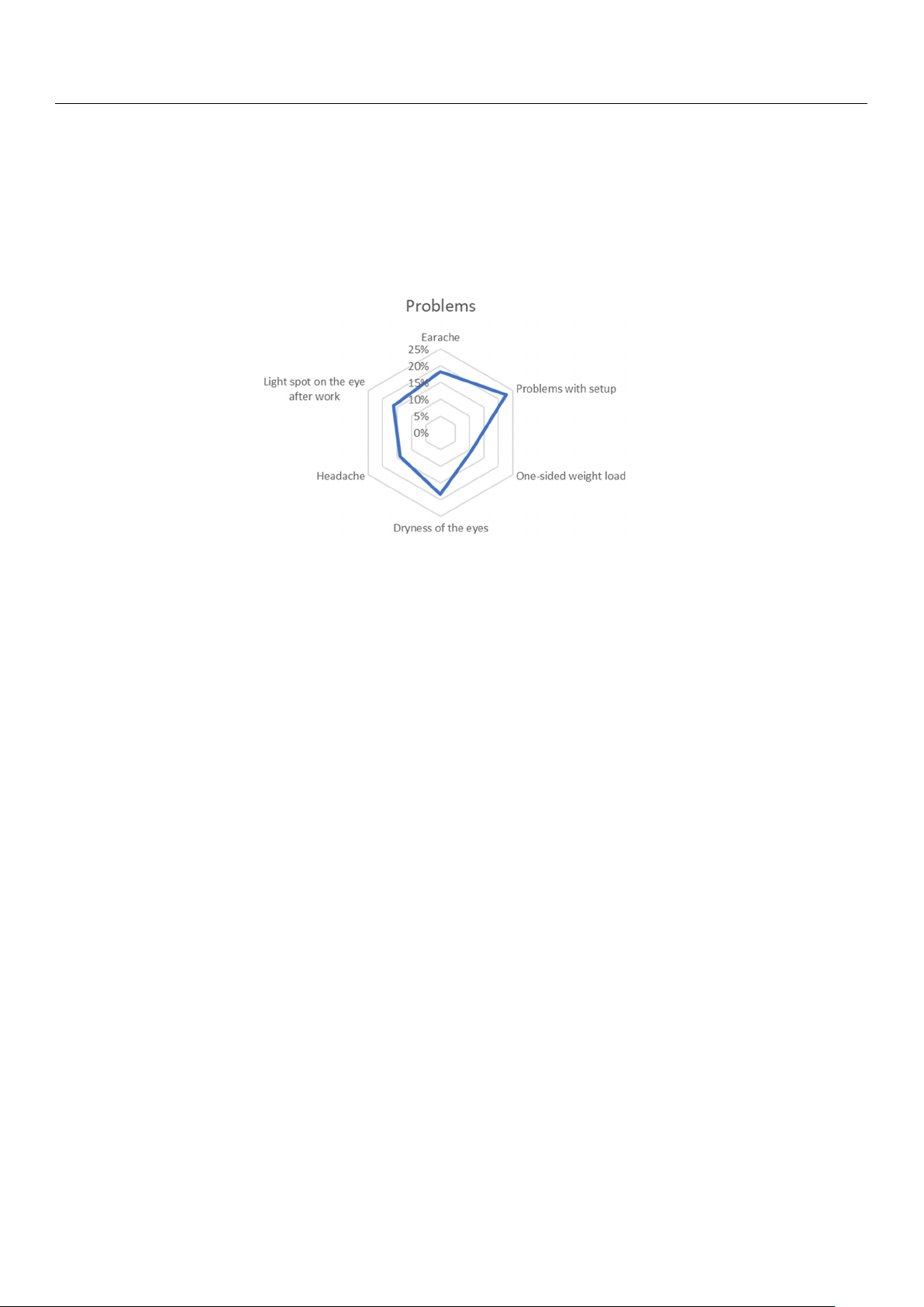
The only open-ended question was about possible concerns regarding the
technology. To analyse this question, the first-order codes were developed us-
ing direct responses, and similar responses were categorised into six concerns as the second-order code. iii.
The interview questions were tested and validated as part of a pilot test
where ten employees of the case company were interviewed, and each gave
individual feedback. The interviews took 10–15 min per interviewee. The
phrasing was improved as an outcome of the pilot. iv.
The inclusion criteria required that the respondents be those who use smart
glasses technology daily or have worked with them in the last year. v.
To assess the broader acceptance of smart glasses, 86 respondents were in-
cluded. They were employees from different companies in the LSP sector.
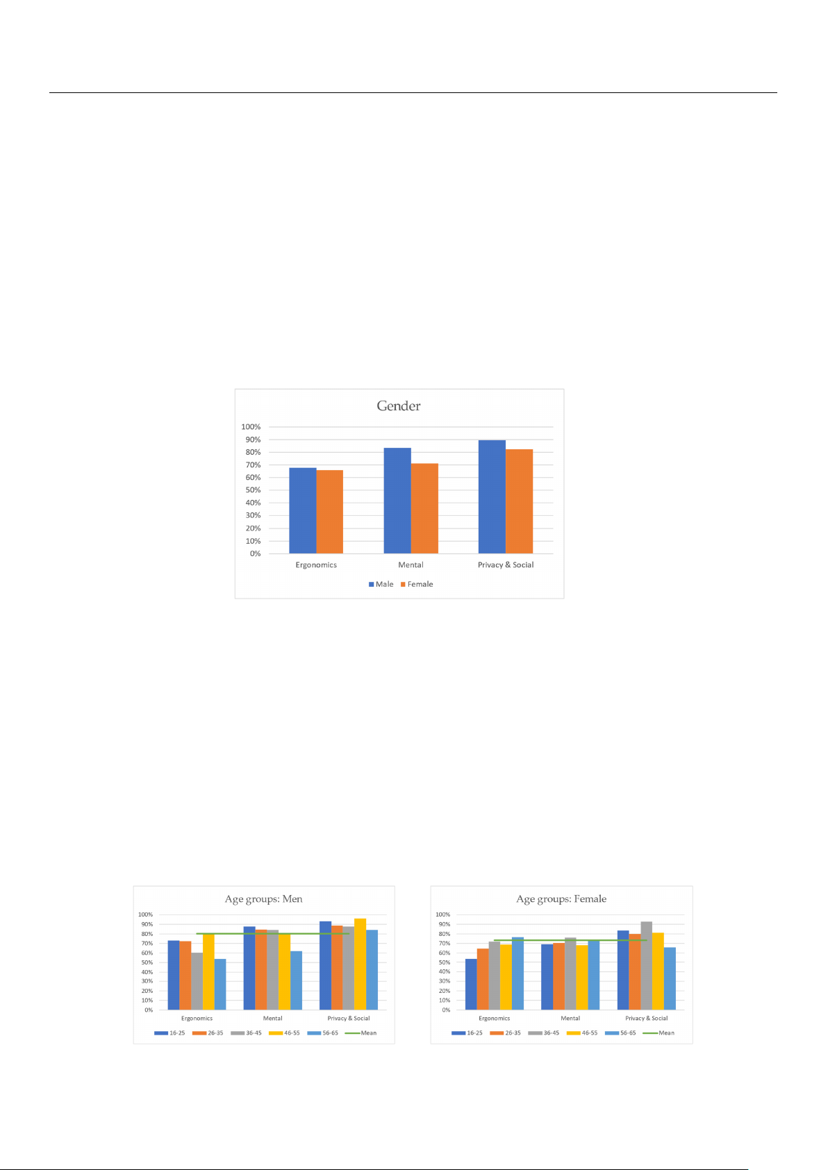
The sample data were divided into 37% women and 63% men. The interviews were conducted face-to-face.
The diversity of the mixed-method approach allowed for rich data collection, which
had the advantage of building a comprehensive view through enhanced triangulation.
These data collection and analysis methods were chosen to achieve the research objectives effectively and objectively.
4. Findings and Discussion
The aim is to achieve the two research objectives in two steps: RO1 is achieved using
the tests performed, regression analysis, scenario analysis, and cost–benefit analysis (CBA),
while RO2 is realised by analysing the data collected through structured interviews.
4.1. RO1: To Assess the Impact of Smart Glasses in Increasing the Effectiveness and Efficiency of
the Picking Processes Compared to Conventional Picking Methods
RO1 is achieved in two parts: (a) first, the ‘efficiency’ part by two test series, regression
analysis, and scenario analysis, and (b) second, the ‘effectiveness’ part via CBA.
4.1.1. Assessing the ‘Efficiency’ of Smart Glasses
To make a scientifically relevant statement about achieving RO1, two different series
of tests were carried out. The first series of tests are based on a test environment outside
the daily business, while the second one is conducted during the live daily business. The
average pick quantity per day based on historical data for the period January–July 2022 is
10,754 picks per day. The average order size based on the total of all orders in 2021 is five
pick positions with three picks each. According to this, a picking activity must be carried out 15 times per order.
Within the pick-by-vision method, the company does not use the option of visual
guidance in route optimisation through the warehouse but a direct location display in the
employee’s field of vision. The smart glasses provide visual information about the storage
location of the material to be picked, the order size, and the respective pick quantity of the
item. To reduce a possible source of error, the order picker confirms the location in advance.
Afterwards, the order picker is provided with the order’s picking information. The scan
confirmation is performed via a scanner integrated into the system, which maintains
Logistics 2024, 8, x FOR PEER REVIEW 9 of 27 Logistics 2024, 8, 106 9 of 25
The scan confirmation is performed via a scanner integrated into the system, which the ma advantage intains th of “hands-fr e advantage ee” or of “h der ands- picking free” or compar der pic ed k to the pick-by-scan ing compar method ed to the pick with -by-scan a hand-held scanner method with a ha . nd-held scanner. T T est est series series 1—pick-by-scan 1—pick-by-sc vs. an vs. pick-by-vision pick-by-vision in in the the test environment: test environm Five ent: Five picking picking processes wer processes wee carried re carr out using ied ou the t usin conventional g the conven pick-by-scan
tional pick-b and pick-by-vision y-scan and pi methods. ck-by-vision Accordingly methods. , the Acco exact rdingl picking y, the locations exact pick wer ing e loc s a tored in tions we the order re stored for in each test the order run for and then each test picked run using and th the pick-by-scan
en picked usin and pick-by-vision g the pick-by-sc methods. an and pi The ck measur -by-visionement period for methods. The the throughput measurement time of a complete period for th order with the respective e throughput time of a
predefined pick quantity starts
complete order with the respective with the predefi order ned pi acceptance ck quantity . It sta ends rts wiwith providing th the order ac the wholly ceptan picked or ce. It ends wi der in the th providi goods ng the issue zone. wholly pi This cked trial series order in thaims to obtain
e goods issu a basic comparison e zone. This trial of seri the es aitechnologies ms to obta based on in a basic throughput comparis time. on of Due to the the technolo standar gies ba disation, it sed on thro is then ughput tpossible ime. to Due make to th a e st statement andardis about ation, it a is potential incr then possibl ease (or e to ma decr ke a ease) stat in ef ement aficiency bout a .
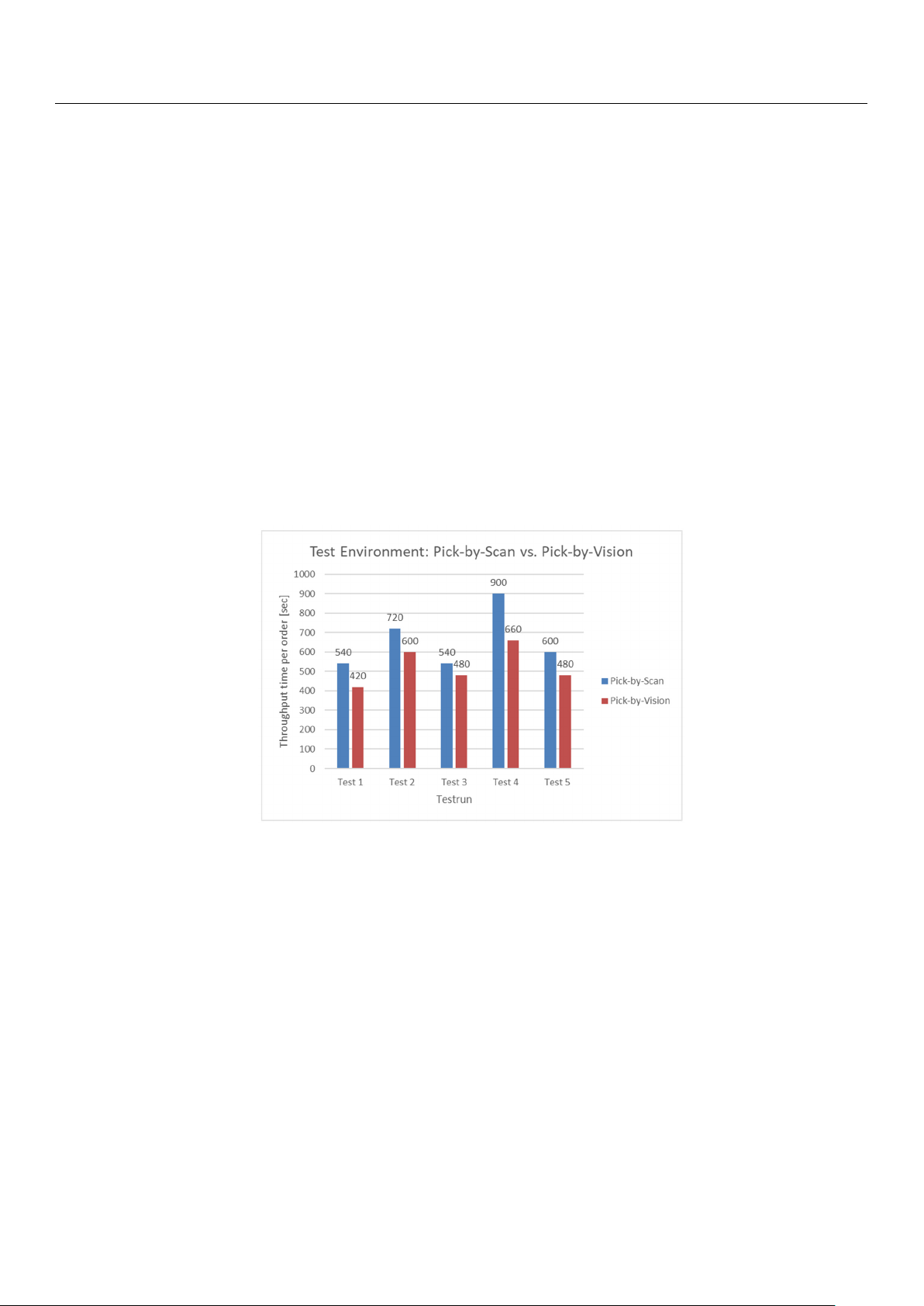
potential increase (or decrease) in efficiency. Figur Figu e re 2 visualises 2 visualises the th thr e th oughput roughput times time of pick-by-scan s of pick-by-sc and an an pick-by-vision d pick-by-visi for on for the the respective respective test series. test seri It can be seen that es. It can be seen th the pick-by-vision at the pick-by-visi method has on method ha a significantly s a significantly shorter throughput time
shorter throughput time in each in ea test series ch test seri compar
es compar ed to the conventional
ed to the conventional pick-by-scan pick-by-scan method. The average method. The av time erage ti per me pick, including per pick, includinsear g sech ar times, ch ti picking mes, picki times, ng ti travel mes, tratimes, vel ti etc., mes, amounts etc., am to 39.76 s with
ounts to 39.76 the conventional s with the conv pick-by-scan entional pi method. ck-by-scan The pick-by-vision method. The pi method ck-by-vision can be quant method ca ified n be her quan e ti with fied an average here with of an av31.81 s per erage of pick. On 31.81 s pe average, r pick. the On av pick-by-vision erage, the pick- method by-vis is ion 7.95 met s h faster od is per 7.95 pick s fa than ster the per conventional pick than pick-by-scan the conventionalmethod, pick-b corr y-sca esponding n method, to a 25% incr correspondi ease in ef ng to a 25 ficiency % in . crease in efficiency. Figure 2. Figure 2.Te T st estenvironm envir ent: co onment: mparison of pi comparison of ck-by-scan and pick-by-scan pick and -by-vision. pick-by-vision. The Thesystem’s performanc system’s e can performance canbe ev be aluated evaluatedbased on based onthe throughp the thr ut ti oughput mes obt times ained obtained in the test en in the test vironment an environment d the respect and the r ive espective pick quantity (F pick quantity igure (Figure 3). The 3). The average orde average or r der picking perf picking ormance wi performance thin the test en within the test vi envir ronment of the pi onment of the ck-by-sca pick-by-scan n method i method is s 95 95.42 .42 picks picks pe per hourr h perour per em employee. ploy The ee. The pick
pick-by-vision -by-vision method method achieves an achieve average s an averag performance e of performa 117.92 nce of picks 11 per 7.92 hour picks per per hour pe employee. r employ The differ ee. T ence in he d the ifference in the performance of perfor the mance o two f systems the two syst amounts toems amo 23.58%. unts t Basedo 23 on .5 a 8%. Based on population of a po 7.48pu h lati per on of shift, 7.48 h p 713.75 er sh picksift, 71 per 3.75 shift pick can s be per shift can achieved be achieved mathematically mathematic per order ally per o picker withrder the picker with the conventional conventional pick pick-by-scan -by- method. The
scan method. The pick-by-vision
pick-by-vision method achieves method a 882.04 chi picks eves per 882.0 shift. 4 picks per shift.
Test series 2—pick-by-scan vs. pick-by-vision in day-to-day operations: The study is
conducted on a sample basis and is intended to represent the population of all orders in the
case company. A sample’s reliability, size, and representativeness play a significant role in
meaningful results [65,66]. The measurement basis of the trial series is based on a total of
10 orders with a total of 105 items and 256 picks of the pick-by-scan method and 12 orders
with 108 items and 367 picks of the pick-by-vision method. One position is equivalent to one picking location. Logistics 2024 Logistics , 20248 , , 8106 , x FOR PEER REVIEW 10 of 10 of 25 27
Figure 3. Order-picking performance per employee (test environment).
Figure 3. Order-picking performance per employee (test environment). Test The ser twoies 2 test —pick series -by-s assistcan in vs. pick-b achieving y-vision RO1 by in day-to-day oper concluding that a ations: The st smart glasses-e udy is nabled conducted on pick-by-vision a samp appr le b oach asis incr and eases is inte the ef nded to repre fectiveness s and ent the population efficiency of the of all o picking r pr ders in ocesses the case compar com ed to pany. A sam conventional ple’s reli picking ability, s
methods.ize, and representativeness play a significant role in R mean egressio in n gfu Ana l re ysi su s: lt T s he [6 c 5, oll6 e6 c ]. Th ted de atmeas a are urement examine basi d for s of nor t m h a e t lit r y ia u l se singrie th s e is K b ol ased mog on orov a – tota Smi l r of 10 nov orders wi test before th a tota further l of 105 analysis. items a The testnd 256 pi assumes cks of in its the pick- null by-sca hypothesis n m that ethod a the nd tested 12 orders wi variable is th 108 i normally tems and 36 distributed. 7 picks of th
The test is e pick-by-vision me
suitable for smaller thod. One po samples (n < sition 30) [ is 67]. equiv The alent to critical one pick value for ing the location.
maximum difference for a sample size (n = 22) at a significance level The two test series of alpha 0.05 [68, assist in 69]. The achiev values ing in T RO1 able by conc 2 show lud thating that a the null smart glasse hypothesis, s-en “a abled normal pick-by-vision distribution appro exists”, ach in cannot creases the e
be rejected. ffectiveness and efficiency of the picking processes
compared to conventional picking methods.
Table Regression Analysis: 2. Kolmogor The
ov-Smirnov test. collected data are examined for normality using the
Kolmogorov–Smirnov test before further analysis. The test assumes in its null hypothesis Kolmogorov-Smirnov Test
that the tested variable is normally distributed. The test is suitable for smaller samples (n
Test Statistics (p-Value)
Critical Value (Quantile K)
< 30) [67]. The critical value for the maximum difference for a sample size (n = 22) at a Throughput Time 0.2016 0.2809
significance level of alpha 0.05 [68,69]. The values in Table 2 show that the null hypothesis, Setup Time 0.0977 0.2809
“a normal distribution exists”, cannot be rejected. Travel Time 0.1002 0.2809 Search Time 0.1743 0.2809
Table 2. Kolmogorov-Smirnov test Pick Time . 0.1664 0.2809
Kolmogorov-Smirnov Test
The next step is identifying the relationship between the dependent and independent
Test statistics (p-value)
Critical Value (Quantile K)
variables through a regression analysis [70]. The dependent variable is the throughput Throughput Time 0.2016 0.2809
time of the picking process. The independent variables directly influencing the throughput time Se ar tup Ti e me setup, travel, search, 0. and 0977 picking times. Table 3 0.2809 illustrates the results from the r Tra egr vel Ti essionme analysis. Multiple 0 R .1002 is 0.9873, indicating a robust 0.2809 linear relationship [71]
between the predictor (independent variables) and the response (dependent: throughput Search Time 0.1743 0.2809
time) variables. The quality of the relationships can be inferred from the R-square of 0.9747, Pick Time 0.1664 0.2809
meaning that the variations in the dependent variable almost wholly explain the variation
in the throughput time. According to [71], 0.05 is a reliable F-value significance level, and the r The egr next ession step is identify table confirms ing the its relation value at sh
0.025.ip between the dependent and independent variables t Regar hrough ding a the regre coef ssion ficients, ana if lys all is [7 other 0]. The pr de edictor pendent v variables a r riable emain is the throughp constant, each ut co- time of the efficient is pick viewed ing as pr the ocess. The average independent increase in the r variab esponse les dir variable ectly for infl each uen unit cing incr the ease throughput time are in a particular pr setup, edictor v travel ariable , sea [72, rch, a 73]. nd pickin Looking at g ti the mes. coef Table 3 ficients, ill it ustrates t becomes he res clear ults that from t the he reg travel ression time (1.160ana 5) lys has is. M the u gr ltiple eatest R is 0.98 positive 73, in corr dicati elation ng a rob with u the st thrlinear rela oughput tionshi time p and [71] betw influences een it the predictor (ind significantly. e However pen , dent v because ar the iables) value isand the above response 1, a certain (dependent: inaccuracy is th pr roughput esent due time) v to ariables. The multicollinearity. qua Thelity of the rel dependent ationships variables can of be travel inferred time (p f = rom the R- 0.0000206), squar sear e ch of 0. time (9 p74 = 7, meaning 0.04511), th and at the v picking ariat time ions (p = in the dependent 0.000000137) corr vari elate able with alm the ost wholly dependent explain the v variable of a thr riation in oughput the throughput time and are time. Accordi statistically ng to [ significant 71] as , 0.0 the 5 p is a reli -values a arb e le F- less value than sign 0.05 i[fic 74 a ].nce lev The el, and variable the regression “setup-time” ( table p = confi 0.8878 rm > s its v 0.05) alue seems at 0. to 025 have. no significant influ-
ence on the throughput time of the process, and this is due to its smaller percentage of time
in the overall picking process.
Logistics 2024, 8, x FOR PEER REVIEW
Logistics 2024, 8, x FOR PEER REVIEW 11 of 27 11 of 27
Logistics 2024, 8, x FOR PEER REVIEW
Logistics 2024, 8, x FOR PEER REVIEW 11 of 27 11 of 27
Logistics 2024, 8, x FOR PEER REVIEW
Logistics 2024, 8, x FOR PEER REVIEW 11 of 27 11 of 27
Logistics 2024, 8, x FOR PEER REVIEW
Logistics 2024, 8, x FOR PEER REVIEW 11 of 27 11 of 27
Table 3. Results of the regression analy sis.
Table 3. Results of the regression analysis.
Logistics 2024, 8, x FOR PEER REVIEW
Logistics 2024, 8, x FOR PEER REVIEW 11 of 27 11 of 27
Table 3. Results of the regression analy sis.
Table 3. Results of the regression analysis.
Logistics 2024, 8, x FOR PEER REVIEW
Logistics 2024, 8, x FOR PEER REVIEW 11 of 27 11 of 27 Regression
Table 3. Results of the regression analy sis. Regr ANOVA ession
Table 3. Results of the regression analysis. ANOVA Regression
Table 3. Results of the regression analysis. Regr ANOVA ession Table 3. Result Sign s of ific the regr anc essi e on analysis. ANOVA Significance Statistic Va Regression lues Item df Statis SS tic Va
Table 3. Results of the regression analysis. Regr ANOVA ession MS lues F Item df SS
Table 3. Results of the regression analysis. ANOVA MS F Sign F ificance Sign F ificance Statistic Va Regression lues Item df Statis SS tic Va
Table 3. Results of the regression analysis. Regr ANOVA ession MS lues F Item df SS
Table 3. Results of the regression analysis. ANOVA MS F Significance Significance Multi Sta pl tis e R tic 0.9872 Va 553 Regression lues 2 Regression 4 1 Sta , Multi2 Item df 9 pl tis 3 e ,37 R tic 0.64 0.9 32 SS Va 3 872 ,34 Regression lues 2.66 5532 ANOVA MS 1 63. 55553 Re 2. gressi5 F 0 × 10 F −13 on F 4 1,2 Item df 93,370.64 32 SS 3,342.66 ANOVA MS 163. 55553 2.5 F 0 × 10−13 Sign F ificance Sign F ificance R-Squa Multi Sta pl tis re 0 e R tic 0 Regr .9 .9 ession 746 872 Va 730 553 lues 6 2 R Reesidual 1 gression 7 4 R- 1 Sta 3 , Multi Item df 3 2p tis ,608 Squa 9l3 e , R tic Regr .3 37 1 re 0 0.64 0.9 .9 3 ession 1 2 SS Va 976 7463 872 , lues ANOVA .9 730 34 553 MS 6 2.66 2 1 63. 55553 Re 2. gressi5 F 0 on 6 Residual 1 × 10⁻¹³ 7 4 1 3, Item df 3 2 ,608 93, .3 37 1 0.64 3 12 SS 976 3, ANOVA .9 34 MS 6 2.66 163. 55553 2.5 F 0 × 10−13 Sign F ificance Sign F ificance Adjus R- Sta t Multi ed Squa pl tis R- re 0 e R tic 0.9 .9746 872 Va 730 553 lues 6 2 R Reesidual 1 gression 7 4 Adjus R- 1 Sta t, Multi ed 3 Item df 3 Squa 29 pl tis R- ,608 3 e , R tic .3 37 1 re 0 0.64 0.9 .9 3 12 SS Va 976 7463 872 , lues.9 730 34 553 MS 6 2.66 2 1 63. 55553 Re 2. gressi5 F 0 on 6 Residual 1 × 10⁻¹³ 7 4 1 3, Item df 3 2 ,608 93, .3 37 1 0.64 3 12 SS 976 3, .9 34 MS 6 2.66 163. 55553 2.5 F 0 × 10−13 Sign F ificance Sign F ificance R-Squa Multi Sta pl tis e R tic 0 re 0.9 . 687 746 872 Va 137 730 553 lues 8 6 2 R Re Tota esi l 21 dual 1 gression 7 4 R- 1, 1 Sta , Multi32 3 Item df 3 29 pl tis 6, Squa3 e 9 , tic 7 ,608 37 R 8. .3 96 0 re 0 0.64 .9 . 687 746 32 872 SS Va 137 1 1976 730 3,34 553 lues 8 .9 MS 6 2.66 2 1 63. 6 55 R Re Tota esi 553 l 2 21 . gressi5 F 0 on dual 1 × 10⁻¹³ 7 4 1, 1,32 3 Item df 3 296, 3 9 , 7 ,608 378. .3 96 0.64 32 SS 3,342.66 MS 163. 55553 2.5 F 0 × 10−13 Square Adjusted R- Square Adjusted R- 1 1976.96 F F R-Squa Multiple R 0 re 0.9 . 687 746 872137 730 5538 6 2 R Re Tota esi l 21 dual 1 gression 7 4 R- 1, 1, Multi32 33 29 pl 6, Squa3 e 9 , 7 ,608 37 R 8. .3 96 0 re 0 0.64 .9 . 687 746 32 872137 1 1976 730 3,34 5538 .96 2.66 2 163. 6 55 R Re Tota esi 553 l 2 21 . gressi50 on dual 1 × 10⁻¹³ 7 4 1, 1,32 33 296, 3 9 , 7 ,608 378. .3 96 1 0.64 3 12976 3, .9 34 6 2.66 163. 55553 2.50 × 10⁻¹³ Standa Sq rd Err uare Adjusted Multiple o R- R r Adjusted R- R-Squa 0 re 0.9 . 687 746 872137 730 5538 6 2 R Re Tota esi l 21 gression 4 Standa Sq rd Err uare dual 17 R- 1, 1, Multi32 33 29 pl 6, Squa3 e 9 , o 7 37 R r ,608 8. .3 96 0 re 0 0.64 .9 . 687 746 32 872137 1 1976 730 3,34 5538 .96 2.66 2 163. 6 55 R Re Tota esi 553 l 2 21 . gressi50 on dual 1 × 10⁻¹³ 7 4 1, 1,32 33 296, 3 9 , 7 ,608 378. .3 96 0.64 323,342.66 163. 55553 2.50 × 10⁻¹³ Square Adjusted R- 44.681535 Square Adjusted R- 44.681535 1 1 976.96 R- (SE Standa ) rd Error Squa 0 re 0.9 . 687 746137 7308 6 R Tota esi l 21 dual 17 R- (SE Standa 1, 3 ) rd Err 32 3 6, Squa 9o 7r ,608 8. .3 96 0 re 0.9 . 687 746137 1 1976 7308 .96 6 R Tota esi l 21 dual 17 1, 32 33 6,97 ,608 8. .3 96 Square Adjusted R- 44.681535 1 1976.96 Square Adjusted R- 44.681535 Observation (SE Standa ) rd Err Adjusted s o R- 22 r 0.96871378 Total 21 (SE Standa 1, ) 326, rd Err 9o 7r 8.960.9687 1378 Total 21 1,326,978.96 Square 44.681535 Observation Adjusted s R- 22 Square 44.681535 Logistics 2024 Standa , 8, 106 (SE) rd Error 0.96871378 Total 21 (SE Standa 1, ) 326, rd Err 9o 7r 8.960.9687 1378 Total 11 of 25 Observations 22 21 1,326,978.96 Square 44.681535 Observations 22 Square 44.681535 Lower Lower Ite Standa m (SE) Co Observation rd Err sor efficients 22 SE t-Sta
t p-value Lower Ite Standa m (SE) rd Error 44.681535 Observation95% Co s Upper effici 95% ents 22 SE Upper 95.0% t-Sta t
p-value Lower 95% Upper 95% Upper 95.0% 44.681535 (SE Standa ) rd Error (SE Standa ) rd Error 95.0 % Lower 95.0 % Lower Item Co Observations efficients
22 SE t-Stat p-value Lower Item 44.681535 Observation95% Co s Upper effici 95% ents 22 SE Upper 95.0%
t-Stat p-value Lower 95% Upper 95% Upper 95.0% 44.681535 Intercept 4 Lower Lower Item (SE) 4 Co .384566 Observations effici 2 ents 132.17 7 0. 22 SE 3357 t-S 97 tat 0.7 p411 3271 Int− e234 Item (SE) .4840 -value Lower 95 3 rcept 4 4 Co 2 Observation95% 3 .384 s effic .i25 566 323 Upper ents − 2 132. 234 17 95 95% .4 .0 841 3 7 0 %. 22 SE 3357 t-Sta 2 t 3.25 322 97 0.7 p 7 411 Upper 95.0% 3271 −234.4840 -value Lower 95 3 2 95% 3.25 323 Upper −234 95 95% .4 .0 841 3 % 23.25 3227
Table 3. Results of the regression analysis. Upper 95.0% Lower Lower Setup Time Inte Item Observation s − rcept 40.642 4 Co .384231 566 effici 6 4 ents . 22 4830 2 132.17 6 −0.143 7 0. SE 3 t-S 257 357 tat 4 0.8 97 0.7 p877 411 712 3276 Int−e10 1 − Ite .10 234 m .4066 Setup Time -value Lower Observation 840 s 24 8 − 95 3 rcept 44 Co . 95% 8 0.642 2 .384161 231 3 effic .i25 566 991 6 4 Upper ents . 22 4 − 323 − 2 132. 10 830 17 95% .10 6 234 95 .4 .0 066 8 −0.143 841 3 7 0 %. SE 3357 t-Sta .t8 2 161 2573.25 991 4 0.8 322 97 0.7 p 4 877 411 Upper 95.0% 712 7 3276 −10 1 − .10 234.4066 840 -value Lower 24 8 95 3 . 95% 8 2 161 3.25 991 Upper − 323 −10 95% .10 234 95 .4 .0 066 8 841 3 % .8 2 161 3.25 991 3224 7 Upper 95.0% 95.0% Lower 95.0% Lower Tra Intercept 4 Item 4 Co .384566 effici 2 ents 132.17 7 0. SE 3357 t-S 97 tat 0.7 p4113271 Int− e234 Item .4840 -value Lower 95 3 rcept 4 4 Co 2 95% 3 .384 effic .i25 566323 Upper ents − 2 132. 234 17 95% .4841 3 7 0. SE 3357 t-Sta 2 t 3.25322 97 0.7 p 7 411 Upper 95.0% 3271 −234.4840 -value Lower 95 3 2 95% 3.25323 Upper −234 95% .4841 323.253227 Upper 95.0% Regression vel Time Setup Time 1−.1605 0.642016 2315 0 6 4.1 .4994 8309 6 5 − .8173 0.143 349 257 2 4 0 ..0 8 6 × 10 877 − 7125 0 Trav 6 − .7 el Ti 10 ANOV 396 me .10066 Setup Time A 14 1−.1 1 24 8.5 605 .8 0.642818 016 161 231391 5 0 6 4.1 991 .4 0 − .7 994 10 830 396 9 .10 6 14 5 − .8 Lower 173 0.143 1 066 8..5 8 257 818 349 161 391 2 4 0 ..0 8 6 991 × 10 4 877 − 7125 0 6 − .7 10 396 .10 14 066 1 24 8.5 .8818 161391 991 0 − .7 10396 .10 14 Lower 1 066 8..5 8 818 161 391 9914 Intercept 4 Item 4 Co .384566 effici 2 ents 132.17 7 0. SE 3357 t-S 97 tat 0.7 p4113271 Int− e234 Item .4840 -value Lower 95 3 rcept 4 4 Co 2 95% 3 .384 effic .i25 566323 Upper ents − 2 132. 234 17 95 95% .4 .0 841 3 7 0 %. SE 3357 t-Sta 2 t 3.25322 97 0.7 p 7 411 Upper 95.0% 3271 −234.4840 -value Lower 95 3 2 95% 3.25323 Upper −234 95 95% .4 .0 841 3 % 23.253227 Upper 95.0% Statistic Search Ti Travel Ti Setup Time V me me alues 0. 1− 5 . 368 1 0.642488 6052317 0165 0 6 4.06..4959 18309 9949 Item 6 05−.7.8713 173 0.143 474 349 257 df 42 4 0 ..5.081 × 10 6 8777126 −10.10066 Setup Time 24 8 − .8 0.642161 231991 6 4.4 −10 830 .10 6 066 8 −0.143 .8161 257 991 4 0.8 4
8777126 −10.1006624 8.8161991 −10.10066 8.81619914 − × 10 2 − 5 Tra SS − v 0.931 Search Ti 0.7 el Ti 558 me 396 me MS 42 2 0. 1 5 14 .1 1.0 368 .5 605052 4887 818 0165 0. 0 6 .1F 562 −0.931 959 391 0. 9 7 9949 95.0 0 3965.. Significance 558 2 %78 713 173 . 14 0 1. 052 474 5 349 4 8182..F 561 505 1 × 10 391 6 − × 10 2 − 5 −0.931 0.7 558 396 42 2 14 1.0 .5052 818562 −0.931 391 0.7 95.0 558 2 396% . 14 0 1. 052 5 561 818 5 391 Trav Int el Ti e me Setup Time 1− rcept 4.14605 0.642 .384016 231 5665 0 6 4.1 .4994 830 2 132.179 6 5−.8173 0.143 7 0.3 349 257 357 2 4 0 .. 97 0. 0876877 411712 3276 Int−e10 1 − .10 234.4066 Setup Time 84024 8 − 95 3 rcept 44 .8 0.642 2 .384161 231 3.25 566991 6 4.4 − 323 − 2 132. 10 830 17 .10 6 234.4066 8 −0.143 841 3 7 0.3357 .8 2 161 2573.25991 4 0.8 322 97 0.7 4 877 411712 7 3276 −10 1 − .10 234.4066 84024 8 95 3.8 2 161 3.25991 − 323 −10.10 234.4066 8 841 3.8 2 161 3.25991 3224 7 − × 10 2 −5 0 Trav .7 el Ti39614 me 1.1 1.5 605818 016391 5 0.1 0.7 994 396 9 14 5.8173 1.5818 349 391 2.06 − × 10 2 −5 0.739614 1.5818391 0.739614 1.5818391 Multiple Pi Inte R ck Ti Search Ti 0.98725532 me me 1 0 rcept 4..0 5 4 777 368 .384119 488 5663 7 00..16 2 132. Regr 068 959 179 9 ession 1 00..082 7713 7 0.3 293 474 357 41 4. 97 0. 3 .5 7 71 411 1,293,370.64 × 10− × 10 8 327 0 Pi − Inte .8 1 − 521 ck Time 0.931 Search Time 234.4 323,342.66 904 558 840 8 1 0 rcept 4..0 5 4 1 42 2 95 3.3 777 .0 368 2 .384032 119 488 3. 5663 0527 25 163.55553 334 0 0..16 0 562 − 323 − 2 132. .8521 068 959 179 0.931 9 234.41 00.7 7 0.3 2.50 905 1 .082 558 2 713 841 3 357 × .3 .0 23 10 474 − 052 13 032 293 .25333 14. 97 0. 3 561 .5 322 7 8 71 × 10 5 − × 10 8 7 411327 0 − .8 1 − 521 0.931 234.4 904 558 840 8 1 42 2 95 3.3 .0 2 032 052 3.25334 0 562 − 323 −.8521 0.931 234.4905 1 558 2 841 3.3 .0 2 032 052 3.25333 561 3228 5 Travel Time Setup Time 1−.1605 0.642016 2315 0 6 4.1 .4994 8309 6 5 − .8173 0.143 349 257 2 4 0 ..0 8 6 × 10 877 7 − 7125 0 Trav 6 − .7 el Ti 10 396 .10 Setup Time 14 me 066 1−.1 1 24 8.5 605 .8 0.642818 016 161 231391 5 0 6 4.1 991 .4 0 − .7 994 10 830 396 9 .10 6 14 5 − .8173 0.143 1 066 8..5 8 257 818 349 161 391 2 4 0 ..0 8 6 9914
8777126 −10.1006624 8.8161991 −10.10066 8.81619914 − × 10 2 −5 0.739614 1.5818391 0.739614 1.5818391 R-Squar Pi e ck Ti Search Ti 0.97467306 me me 1 0..05777 368119 4883 7 00..16 Residual 068 9599 9 100..082 7713293 474 1714.3 .571 × 10− × 10−233,608.31 8 0 Pi − .8521 ck Ti 0.931 Search Ti 904 me 558 me 1976.96 8 1 0..05 1 42 2.3 777 .0 368032 119 052 488334 3 7 00..16 0 562 −.8521 068 9599 0.931 9 905 1 00.7 1 .082 558 2 713 .3 .0032 293 052 474 333 14.3 561 .58 71 × 10 5 − × 10 8 0 − .8521 0.931 904 558 8 1 42 2.3 .0032 052334 0 562 −.8521 0.931905 1 558 2.3 .0032 052333 5618 5 Travel Time Setup Time 1−.1605 0.642016 2315 0 6 4.1 .4994 8309 6 5 − .8173 0.143 349 257 2 4 0 ..0 8 6 8777126 −10.10066 Setup Time 24 8 − .8 0.642161 231991 6 4.4 −10 830 .10 6 066 8 −0.143 .8161 257 991 4 0.8 4
8777126 −10.1006624 8.8161991 −10.10066 8.81619914 − × 10 2 −5 0 Trav .7 el Ti39614 me 1.1 1.5 605818 016391 5 0.1 0.7 994 396 9 14 5.8173 1.5818 349 391 2.06 − × 10 2 −5 0.739614 1.5818391 0.739614 1.5818391 Adjusted Pick Time Search Time 1 0..05777 368119 4883 7 00..16068 9599 9 100..082 7713293 474 14.3 .571 × 10− × 10 8 0 Pi − .8521 ck Ti 0.931 Search Ti 904 me 558 me 8 1 0..05 1 42 2.3 777 .0 368032 119 052 488334 3 7 00..16 0 562 −.8521 068 9599 0.931 9 905 1 00.7 1 .082 558 2 713 .3 .0032 293 052 474 333 14.3 561 .58 71 × 10 5 − × 10 8 0 − .8521 0.931 904 558 8 1 42 2.3 .0032 052334 0 562 −.8521 0.931905 1 558 2.3 .0032 052333 5618 5 Travel Ti 0.96871378 me 1.16050165 0.1Reg 994 T a 9 otal rding th 5.8173349 21 e coeffi 2. ci 0 ent 6 s 1,326,978.96 , if a − × 10 2 −5 Tra ll ot 0 v . her 7 el Ti396 me predict 14 1.1 o 1. r v 5 605 a 818 016 ri 5 abl 0. e 1 s rem Reg 391 0.7 994 a 9 a 396 i rd5 n . const ing th 14 8173 1. a 5 349 nt, e e coeffi 8182. a 0 ch cient 6 s, 391 if a − × 10 2 −5 ll ot 0. her 7396 predict 14 o 1. r v 5 a 818 riables rem 391 0.7 a 396 in const 14 1. a 5 nt, e 818 ach 391 R-Squar Pi e ck Time Search Time 1 0..05777 368119 4883 7 00..16068 9599 9 100..082 7713293 474 14.3 .571 × 10− × 10 8 0 Pi − .8521 ck Ti 0.931 Search Ti 904 me 558 me 8 1 0..05 1 42 2.3 777 .0 368032 119 052 488334 3 7 00..16 0 562 −.8521 068 9599 0.931 9 905 1 00.7 1 .082 558 2 713 .3 .0032 293 052 474 333 14.3 561 .58 71 × 10 5 − × 10 8 0 − .8521 0.931 904 558 8 1 42 2.3 .0032 052334 0 562 −.8521 0.931905 1 558 2.3 .0032 052333 5618 5 coefficient is Regard viewed ing th as the e coeffi av ci er ent ag s,− e 2 incre if a ase ll ot in her the response v predictor vari ar coei ablab ffi e le fo Rega r e cient is s remai rd a nch un view ing th it incre ed const as the ant, e e coeffi a cise aver ch ent ag s,− e 2 incre if a ase ll ot in her the response v predictor vari ari ablab e le for e s remai a nch unit incre constant, e ase ch Standar Pi d ck Time Search Time 1 0..05777 368119 4883 7 00..16068 9599 9 100..082 7713293 474 14.3 .571 × 10− × 10 8 0 Pi − .8521 ck Ti 0.931 Search Ti 904 me 558 me 8 1 0..05 1 42 2.3 777 .0 368032 119 052 488334 3 7 00..16 0 562 −.8521 068 9599 0.931 9 905 1 00.7 1 .082 558 2 713 .3 .0032 293 052 474 333 14.3 561 .58 71 × 10 5 − × 10 8 0 − .8521 0.931 904 558 8 1 42 2.3 .0032 052334 0 562 −.8521 0.931905 1 558 2.3 .0032 052333 5618 5 44.681535 in a coe part ffi ic Rega ul rda cient is r predict viewed ing th or e coe va as the ffi riab av cientle ers, [7 ag 2, e 7 if a 3]. incre Lookin ase ll ot in her g at the t predicthoe coe r varffi response v i c a i in a r coe ablent iab ffi e s, it become partic Rega ul le fo s rema rda r e cient is i ra nch view ing th s un constclear that predict ed a or nt e coe va it incre as the , e ffi riab a cise av ch entle ers, [7 ag 2, e 7 if a 3]. incre Lookin ase ll ot in her g at the t predicthoe coe r varffi response v i c a i r ablent iab e s, it become le for e s remai a nch s un constclear that it incre ant, e ase ch Error Pi (SE) ck Time 1.07771193 0.10689 10.082293 1.37 × 10⁻⁸ 0 Pi .8521 ck Ti 904 me 8 1.0 1.3 777032 119334 3 0.1 0.8521 0689 905 10 1 .082 .3032 293 333 1.38
7 × 10⁻⁸ 0.85219048 1.3032334 0.8521905 1.30323338 in a coe part ffi ic Rega ul rda cient is r predict viewed ing th or e coe va as the ffi riab av cientle ers, [7 ag 2, e 7 if a 3]. incre Lookin ase ll ot in her g at the t predicthoe coe r varffi response v i c a i in a r coe ablent iab ffi e s, it become partic Rega ul le fo s rema rda r e cient is i ra nch view ing th s un constclear that predict ed a or nt e coe va it incre as the , e ffi riab a cise av ch entle ers, [7 ag 2, e 7 if a 3]. incre Lookin ase ll ot in her g at the t predicthoe coe r varffi response v i c a i r ablent iab e s, it become le for e s remai a nch s un constclear that it incre ant, e ase ch Observations 22
the travel time (1.1605) has the greatest positive correlation with the throughp the travel time (1 ut ti .1605 me ) haan s d
the greatest positive correlation with the throughput time and coefficient is Regard viewed ing th as the e coeffi av ci er ent ag s, e incre if a ase ll ot in her the response v predictor vari ar coei ablab ffi e le fo Rega r e cient is s remai rd a nch un view ing th it incre ed const as the ant, e e coeffi a cise aver ch ent ag s, e incre if a ase ll ot in her the response v predictor vari ari ablab e le for e s remai a nch unit incre constant, e ase ch influences it the tra in a vel ti particul signi m aer (1 ficant .1605 predict)oly r . ha How s variab ev le er, the grea [72,b7e3ca test p ]. u o s si e ti tvh e e Lookin val g at u t e correla h is ti ab e coe ov in on wi ffi e 1, fl the tra ci in a a v ents part ce ic rt uences it el ti ul ain m aer inac signi (1 fi th the throughp .16 , it becomes curac cant ut ti 05 predict)oly r . me hav y a s is How nd clear that riab ev le er, the grea [72,b7e3ca test p ]. u o s si e ti tvh e e Lookin val g at u t e correla h is ti ab e coe ov on wi ffi e 1, ci a ents certain inac th the throughp , it becomes curac ut time y a is nd clear that Item Coefficients SE coeffiReg t-Stat cient is ard viewed ing th p-value as the e coeffi av ci er ents Lower ag , e if a 95% increase ll ot Upper in her the 95% predictor vaLower response v ri ar coeiffi able 95.0% able fo Rega r e cient is s remai rd a n Upper ch un viewed const ing th 95.0% it incre as the ant, e e coeffi a cise aver ch ent ag s, e incre if a ase ll ot in her the response v predictor vari ari ablab e le for e s remai a nch unit incre constant, e ase ch influences it the tra in a vel ti particul signi m aer (1 ficant .1605 predict)oly r . ha How s variab ev le er, the grea [72,b7e3ca test p ]. u o s si e ti tvh e e Lookin val g at u t e correla h is ti ab e coe ov in on wi ffi e 1, fl the tra ci in a a v ents part ce ic rt uences it el ti ul ain m aer inac signi (1 fi th the throughp .16 , it becomes curac cant ut ti 05 predict)oly r . me hav y a s is How nd clear that riab ev le er, the grea [72,b7e3ca test p ]. u o s si e ti tvh e e Lookin val g at u t e correla h is ti ab e coe ov on wi ffi e 1, ci a ents certain inac th the throughp , it becomes curac ut time y a is nd clear that Intercept 44.3845662 132.177 coeffi 0.335797 present due to cient is view 0.74113271 multicollineari ed as the aver − ag234.484095 ty. The de e increase in 323.25323 pendent vari the − response v 234.4841 ables of travel time present due t ( o ar coeiab ffi le for e cient is a 323.253227 p = 0. mult 0000206 icollin ),
earity. The dependent variables of travel time (p = 0.0000206), ch un view it incre ed as thease
average increase in the response variable for each unit increase influences it the tra in a vel ti particul signi m aer (1 ficant .1605 predict)oly r . ha How s variab ev le er, the grea [72,b7e3ca test p ]. u o s si e ti tvh e e Lookin val g at u t e correla h is ti ab e coe ov in on wi ffi e 1, fl the tra ci in a a v ents part ce ic rt uences it el ti ul ain m aer inac signi (1 fi th the throughp .16 , it becomes curac cant ut ti 05 predict)oly r . me hav y a s is How nd clear that riab ev le er, the grea [72,b7e3ca test p ]. u o s si e ti tvh e e Lookin val g at u t e correla h is ti ab e coe ov on wi ffi e 1, ci a ents certain inac th the throughp , it becomes curac ut time y a is nd clear that Setup Time −0.6422316 4.48306 search −0.1432574 time present du (p e t = o 0.0 0.88777126 451 mult 1), a icollinnd pi eari −10.1006624 cking ti ty. The m de e (p 8.8161991 = 0.0000 pendent var 00 i 137 −10.10066 ) correla search ables of trav te wi time present du (p el time e t ( o 8.81619914 th the dependent = 0 p .0 = 451 0. mult 0 1), 000 a icollinn 206 ear d pi ), i cking ti ty. The m de e (p = 0.0000 pendent var 00 i 137) correla
ables of trav te with the dependent el time (p = 0.0000206 ), influences it the tra in a vel ti particul signi m aer (1 ficant .1605 predict)oly r . ha How s variab ev le er, the grea [72,b7e3ca test p ]. u o s si e ti tvh e e Lookin val g at u t e correla h is ti ab e coe ov in on wi ffi e 1, fl the tra ci in a a v ents part ce ic rt uences it el ti ul ain m aer inac signi (1 fi th the throughp .16 , it becomes curac cant ut ti 05 predict)oly r . me hav y a s is How nd clear that riab ev le er, the grea [72,b7e3ca test p ]. u o s si e ti tvh e e Lookin val g at u t e correla h is ti ab e coe ov on wi ffi e 1, ci a ents certain inac th the throughp , it becomes curac ut time y a is nd clear that Travel Time 1.16050165 0.19949 variab search 5.8173349 le of t time present du h (p e t = o 0.02.06 roughp 451 mult × ut t 1) i10 icollin − , an 5 med pi eari 0.739614 and a ckire st n ty. The at g ti de ist me i ( ca p 1.5818391 ll = y s 0.0 i pendent v gn 000 ari ifi 00137 v0.739614 cant as the ariab ) correla search ables of trav p-v present dualue le of t time h te wi (p el time e t = ( o 1.5818391 s ar 0 p .0 = e less tha roughp 0. mult ut 451 0 t 1) i 000m , a icollin e n 206n th the dependent ear and a d pi ), i ckire st n ty. The at g ti de ist me i ( ca p ll = y s 0.0 i pendent v gn 000 ari ifi 00cant as the 137) correla ables of trav p-value te wi el time ( s ar p = e less tha 0.0000206n th the dependent ), present d infl the trav ue t uences it el timoe mult signi (1 fi .16 icollin cant 05) ly. ha ear s ity. The However, the grea d beecpendent v a test p u o s si e ti tvh e e varliables of trav ue correla is ti abov infl on wi the trael time present d e 1, a v ue t cert uences it el tim ( o e p ain (1= signi 0 fi th the throughp .16 . mult 0 inac0 000 cant ut ti 5) l 206 icollin curac y. me ha y an s ), earity. The is How d ever, the grea d beecpendent v a test p u o s si e ti tvh e e varliables of trav ue correla is ti abov on wi el time e 1, a cert (p ain = 0 th the throughp .0 inac 000 ut ti 206 curac me y an), is d Search Time 0.53684887 0.69599 0. v 05 ari [7 ab search 0.7713474 4]. Th le of t time ( e v hp = a 0.04.51 roughp 451 × riable ut t 1) i10− , an 2 med pi − “setup-t 0.93155842 im and a cki e” rn ( e st g tip atist me i ( ca p 2.0052562 ll = y s 0.0 ign 000 ifi 00137 − = 0.8878 > 0.05 0. v 0.931558 ) seem 05 ari s to ha [7 ab search 4] cant as the ) correlap-v le of t time v . Th te wi ( e alue hp 2.00525615 no si e v = a0ri s ar .0 gni ab roughp le ut 451 fi t 1) i, cant “s aet me n up e less than th the dependent -t d pi im and a cki e” rn ( e st g tip at m = 0.887 ist e i ( ca p ll = 0.8 y s 0 > i 0.05 gn 000 ifi 00 ) seem 137 s to ha cant as the ) correlap-v v te wi e no si alues ar gnificant e less than th the dependent present d infl ue t uences it o mult signifi icollin cantly. earity. The However, d beecpendent v ause the varliables of trav ue is abov infl el time present d e 1, a ue t cert uences it ( o p ain = signi 0 fi . mult 0 inac 000 cantl 206 icollin curac y. y ), earity. The is However, d beecpendent v ause the varliables of trav ue is abov el time e 1, a cert (p ain = 0.0 inac 000206 curacy ), is Pick Time 1.07771193 0.10689 0. v 05 ari [7 ab search 10.082293 4]. Th le of t time ( e v hp = a 0.01.37 riab roughp 451 × le ut t 1) i10 , a − n 8 “set meup-t d pi 0.85219048 im and a cki e” rn ( e st g tip atist me i ( ca p 1.3032334 = 0.887 ll = 0.8 y s 0 > i 0.05 gn 000 ifi 00137 0.8521905 ) seem 0. v 05 ari s to ha [7 ab search 4] cant as the ) correlap-v le of t time v . Th te wi ( e alue hp 1.30323338 th the dependent = 0.04511), an
d picking time (p = 0.000000137) correlate with the dependent
influence on the throughput time of the process, and this is d inu fle to its smaller uence on th e va per no si ri s arab roughp c utentage e throughput time of the gni le fi ti cant “set meup e less than -tim and a e” r ( e st process, p at = 0.887 isticall and t 8 y s > i gn h i is is d 0.05 fi ue to its smaller ) seems to ha cant as the p-v ve alue per no si s ar centage gnificant e less than variable of t search time present du h ( e troughp p = o 0.0 mult ut 451 t 1) im , a icollin e n and a d pi eari ckire st n ty. The at g ti de ist me i ( ca p ll = y s 0.0 i pendent v gn 000 ari ifi 00cant as the 137 variab ) correla search ables of trav p-v present dualue le of t time h te wi (p el time e t ( o s ar = 0 p .0 = e less tha roughp 0. mult ut 451 0 t 1) i 000m , a icollin e n 206n th the dependent ear and a d pi ), i ckire st n ty. The at g ti de ist me i ( ca p ll = y s 0.0 i pendent v gn 000 ari ifi 00cant as the 137) correla ables of trav p-value te wi el time ( s ar p = e less tha 0.0000206n th the dependent ), of time in 0. fl 05 [7 in the uence on t 4]. Th ov h erall pic e variable k in “s g process. e throughput time of the etup-time” ( process, p = 0.887 and t 8 > h 0.05 of time is is d in 0. u fl ) seem 05 [7 in the uence on t s to ha 4] v . Th ov h e erall pic e to its smaller e va per no si riab c gni le kfi in “s g process. entage e throughput time of the cant etup-time” ( process, p = 0.887 and t 8 > his is d 0.05 ue to its smaller ) seems to have per no si centage gnificant variable of t search time h ( roughp p = 0.0 ut 451 t 1) im , a e n and a d pickire st n at g ti ist me i ( ca p ll = y s 0.0 ign 000 ifi 00cant as the 137 variab ) correla search p-value le of t time h te wi (p s ar = 0.0e less tha roughput 451 t 1) im , a e n n th the dependent and a d pickire st n at g ti ist me i ( ca p ll = y s 0.0 ign 000 ifi 00cant as the 137) correlap-value te wi s are less than th the dependent of time in 0. fl 05 [7 in the uence on t 4]. Th ov h erall pic e variable k in “s g process. e throughput time of the etup-time” ( process, p = 0.887 and t 8 > h 0.05 of time is is d in 0. u fl ) seem 05 [7 in the uence on t s to ha 4] v . Th ov h e erall pic e to its smaller e va per no si riab c gni le kfi in “s g process. entage e throughput time of the cant etup-time” ( process, p = 0.887 and t 8 > his is d 0.05 ue to its smaller ) seems to have per no si centage gnificant 0. varThe 05i [7 ab r 4]egression The regressio . Th le of t e v h a analysi n analy riab roughp le ut ti ss “s m further eteup-tim and ar helps e” ( e stp at explain is further helps expl = 0.887 isticall RO1, ain RO 8 y s > i gnifi concluding 1, concludi 0.05) seem 0. v 05 ari [7 cant as the ab that ng th s to ha 4]. Th p-v le of t optimising at opti The regressio m n isi ve h no si e v alue ari s ar gni ab roughp le ut t the ng t analys he
is further helps explain RO1, concluding that optimising the infl fiicant “set meup e less than -tim and a e” r ( e stp at = 0.887 isticall 8 y s > i 0.05 gnifi ) seems to ha
cant as the p-v ve no si alues ar gnificant e less than The regressio of time in the uence on tov h n analy erall pick sis further helps e ing process. e throughput time of the xplain process, RO and t 1, c h onclud is is d inu fl ing t of time hat in the uence on t op ov h t e to its smalleri The regressio m n is per icng erall pick t analys h in e is further helps e g process. entage e throughput time of the xplain process, RO and t 1, c h onclud is is du ing that opt e to its smallerimis per icng the entage independent in 0. fl 05 [74] variables independent vari uence on t . Th h e vari can able change ables ca “setup the -tim thr e” oug e throughput time of the (p hput time process, = 0.8878 > and and t h 0.05incr 0.ease is is d inu fl ) seem 05 [ ef 7 fi 4] ciency independent v uence on t s to hav . Th h e .a e vIn
n change the throughput time and increase eri e to its smaller aricontinua- fficiency. In
ables can change the throughput time and increase efficiency. In per no si ab centage e throughput time of the gni le fi cant “setup-time” ( process, p = 0.887 and t 8 > his is d 0.05 ue to its smaller ) seems to have per no si centage gnificant independent of time v in the a ovriables c The regression erall pic a analy
k n change the throughput time and increase e sis further helps e ing process. xplain RO1, c independent oncluding t of time h v at in the a ovrffi i opti The regressio c n i mency. In ables c isi erall pic a ng analy
k n change the throughput time and increase e t s h in e is further helps e g process. xplain RO1, concluding that ffi opti ci mency. In ising the tion, infl these continua of time same in the uence on th variables tion, these sa overall pic wer kin e me va influenced riables we g process.
e throughput time of the heavily re infl process, by the and th pick-by-vision uenced heavily b contin y ua of time is is d inu fl app in the uence on tov h roach, the pick-b tion, these sa e to its smaller perc thus y-vision me v
ariables were influenced heavily by the pick-by-vision erall picking process. entage
e throughput time of the process, and this is due to its smaller percentage continuation, these sa independent vari The regression me v ables ca analys ariables were is further helps e in x fl pl uenced heavily b ain RO1, c conti o n ncludi y ua the pick-b
n change the throughput time and increase e independent ng th v at arffi i opti The regressio c n i m y-visio tion, these sa ables c isi a ng t analys n me v h aria ency. In e bles were is further helps e in x fl pl uenced heavily b ain RO1, concludi y the pick-b
n change the throughput time and increase e ng that ffi opti ci m y-visio ising t n h ency. In e achieving of time higher approach, th in the ef ov ficiency erall pic .
us achieving higher efficiency.
approach, thus achieving higher efficiency. king process.
of time in the overall picking process. continuation, these sa independent vari The regression me v ables ca analys ariables were is further helps e in x fl pl uenced heavily b ain RO1, c conti o n ncludi y ua the pick-b
n change the throughput time and increase e independent ng th v at arffi i opti The regressio c n i m y-visio tion, these sa ables c isi a ng t analys n me v h aria ency. In e bles were is further helps e in x fl pl uenced heavily b ain RO1, concludi y the pick-b
n change the throughput time and increase e ng that ffi opti ci m y-visio ising t n h ency. In e Scenario Scenari approach, th Analysis: o Analysis The regression The us achieving analys data sets : The data higher effici aggr ency egated sets aggrega . t is further helps expl to ain a ROmean ed to a me 1, co value, an va ncludi and lue, Scenari approach, o th ng th the at op r ti The regressio espective and the respe Analysis c us achieving tive : The data sets aggrega higher efficiency.
ted to a mean value, and the respective m n ising t analys he
is further helps explain RO1, concluding that optimising the approach continua , thus achieving tion, these sa independent vari higher e me v ables ca aria ffi b cienc les w y e . re infl approach uenced heavily b contin y ua , thus achieving the pick-b tion, these sa
n change the throughput time and increase e independent varffi i ci higher e y-visio ables ca n me v aria ency. In ffi b cienc les w y e .
re influenced heavily by the pick-b
n change the throughput time and increase effici y-vision ency. In standar stand d a deviation rd dev Scenari i o independent var of ation Anal i the of ysis test the ables ca series test se : The datacan ries cbe an seen in sets aggrega T be seent able in T 4 a . This ble 4. ed to a me data stand an vaset This da ard serves ta s lue, e Scenarit se devi o independent v as rv
n change the throughput time and increase e ari a ation Anal ffi basis es as of the and the respe ysis ci ables cfor a bcasi tivs test se e rie : The data s can be seen sets aggrega in t Table 4. ed to a m This d ean va ata s lue, et serves as a b and the respecasi tivs e ency. In
an change the throughput time and increase efficiency. In Scenari approach continua , o th Analysis: The data us achieving
tion, these same varia sets aggrega higher effi b cienc les w y e . re in ted to a m fl ean va conti lue, approach uenced heavily b n y ua , and the respe Scenario th Analysi the pick-b s tion, these sa c us achieving tiv y-visio en me v : The data aria sets aggrega higher effi b cienc les w y e . re in ted to a m fl ean value,
uenced heavily by and the respe the pick-b ctiv y-visio en further for stand conti analyses. further ard devi nua Based analys ation of on es. tion, these sa the Base the collected d on test series c me variab data the co an les we and re i determined llected dat be seen in a Table nfl time 4. for elements and determ stand in further This da a ta s rd e dev uenced heavily b contin y ua in t se i combination ed time e analy rv l s ation e es m of ents i es. Base as a b the as n i d on s the co test series canllected dat be seen in a T and determ able 4. in This da ed time ta set se e rv le es ments i as a bas n i s the pick-by-visio tion, these sa n me v
ariables were influenced heavily by the pick-by-vision standard dev Scenari approach, th i o ation Anal of the ysis us achieving test serie : The data higher e s c ffi a ci n en be seen sets aggrega cy. in t Table 4. ed to a m This d stand ean va a a ta s rd lue, approach, e Scenarit se dev th i o rves ation Anal as of ysisa b the and the respec us achieving asi tivs test se e rie : The data higher e s c ffi a ci n en be seen sets aggrega cy. in t Table 4. ed to a m This d ean va ata s lue, et serves as a b and the respecasi tivs e with the for historical combination further wit approach, th data h analy t s h r es. ecor e hist us achieving ds Base fr orica om l d d on a higher e 2021, ta re the co fficien scenarios cords llected cy. wer from 2 dat 0 a e 2 cr 1, eated scenarin and determ for which ios w in e combinat further approach, th dif ion f re cre ed timeer a wit t h analy ent e esd th le or m es. ders in wh e hist ich orica ents i Base n l d d on ata records the co from llected 2 dat 0 a 2 1, scenarios and determ w in ere crea ed time te ed l in wh em ich ents in
us achieving higher efficiency. for further standard Scenarianaly devi o ses. ation Anal of ysi Base the s d on the co test serie : The data s canllected sets aggrega dat be seen in t a T and determ able 4. ed to a m for stand ean va in This da a ed time further ta s rd lue, e Scenarit se devi o e analy rv l s ation Anal e es m of ysi ents i es. Base as sa b the and the respecas n i tive d on s the co test serie : The data s canllected sets aggrega dat be seen in t a T and determ able 4. ed to a mean va in This da ed time ta s lue, et se e rv le es ments i as a b and the respecas n i tive s with di dif ff ferent combinat Scenari picking erent orders wi ion with t o Anal positions th di h ff e hist ysis wer orical e erent pi da : The data estimated. cki t n a g re positi cords In sets aggregateach ons w from e 2 case, 021, the re estidi scen ed to a me pick maff arios an va quantity ted. In ea we combinat re cre ion lue, Scenario is a wit t hmultiplied ch case, the pi erent orders wi e tth di dh ff in wh e hist ck erent pi ich orical dcki at n a g re positi cords ons w from e 2 re esti 021, ma scen ted. In ea arios we ch ca re creat se, the pi ed in wh ck ich and the respe Analysis ctive
: The data sets aggregated to a mean value, and the respective combinat for standard ion further wit devi h analy t s ationhe hist es. of the orica Base l d d on test se at rie a s re ca cords the co n from llected be seen in 2 dat 0 a T 2 a 1, scen ble 4. arios and determ for This d standa w in ard e combinat re cre ion further ta set se devi a wit ed time t rve h e analysd tl ation in wh h e es e hist m es. as of a b the ich orica ents i Baseas n is l d d on test se at rie a s re ca cords the co n from llected be seen in 2 dat 0 a T 2 a 1, scen ble 4. arios and determ This d w in a ere cre ta set se a ed time t rve ed l in wh e es m as a b ich ents i as n i s by q the u di a ff n pick ti standard position ty is multip devi by li erent orders wi ation of a factor ed by t th diff h the of e pi test se 3 erent pi (average cking ries can pick positi be seen quantity ons we in Table per
ck position by a factor of 3 (a re esti v q 4. pick e u di ra a maff nti This d standaposition ge pick ty is m ted. In ea ul ata s rd e devi in quatn ip t serv 2021). t ch ca ili erent orders with di es ation as of The ty per pic ed by t ff h se, the pi k e pi
ck ck position by a factor of 3 erent picking positions we (a re esti vera ma ge pick qua ted. In ea nt ch ca ity per pic se, the pi k ck a b the asis
test series can be seen in Table 4. This data set serves as a basis different orders wi combinat for ion further with analy t s th di h es. fferent pi e historica Base l d d on cki at n a g re posi the co ti cords ons w from llected dat e 2a re esti 02 1, ma di scen ted. In ea ff arios and determ for w in e combinat further ch ca re cre ion a wit ed time th analyse, the pi erent orders wi e t es th di dh lem es. ff in wh e hist Base ck erent pi ich orica ents in l d d on cki at n a g re posi the co ti cords ons w from llected dat e 2a re esti 02 1, ma scen ted. In ea arios and determ w in e ch ca re crea ed time tse, the pi e ed l in wh em ck ich ents in data qu sets anti of position the in ty is m scenarios 2021). ulti The pli can data ed by t be h found sets o e pi f in the Appendix scenarios c B a . n The be specific found
ck position by a factor of 3 (aq in ve ua scenario position ranti in ge pick ty is m for Appendix qua ultifive B. 2021).nt p ili picking The speci dat ty per a ed by t fi pic h c sets o k
e pi f the scenarios can be found
ck position by a factor of 3 (a in ve Appendix rage pick B. qua The nti speci ty per fi pic c k different orders wi combinat for ion further with analy t s th di h es. fferent pi e historica Base l d d on cki at n a g re posi the co ti cords ons w from llected dat e 2a re esti 02 1, ma di scen ted. In ea ff arios and determ for w in e combinat further ch ca re cre ion a wit ed time th analyse, the pi erent orders wi e t es th di dh lem es. ff in wh e hist Base ck erent pi ich orica ents in l d d on cki at n a g re posi the co ti cords ons w from llected dat e 2a re esti 02 1, ma scen ted. In ea arios and determ w in e ch ca re crea ed time tse, the pi e ed l in wh em ck ich ents in positions scenar quanti with io for position in thr fi ty is m v u eltee pi 2021). ip picks cki li n The each g posi data ed by t h can ti sets o e pi be f taken ons wi the sce fr n om th three pi ario Table cks ea s can 5, be wher ch can
ck position by a factor of 3 (aqe foundve u the be scenar in ra antief ioficiency taken from for position in fi ge pick ty is m v u e Appendix qua lt is Ta pi B. 2021).n i t p impr ble cki ili n The oved 5, whe speci dat ty per a ed by t h r pice g posi fik ti ons wi c sets o e pi f th three pi the scenario cks ea s can ch can be
ck position by a factor of 3 be found (ave taken from in rage pick T Appendix quaa B.nble ti 5, whe The speci ty per r pice fik c qu di a ff ntity is m combinat u ion lti witphli erent orders wi ted by t th di h ff e histhe pi
oricack position by a factor of 3 erent pi l dcki at n a g re positi cords ons w from e 2021, (a re esti v q e u di scen ra a maff ar ge pick nti ios we combinat qua ty is m ted. In ea u ion lt re cre n ia wit t p ch cat h iety per li erent orders wi tth di dh pic ed by t ff e histh se, the pi in wh k e pi ck ich
oricack position by a factor of 3 erent pi l dcki at n a g re positi cords ons w from e 2021, (a re esti ve scen ra ma ar ge pick ios we qua ted. In ea re cre n a t ch cat iety per d pic se, the pi in wh k ck ich by 10% the e for ffi scenar ci io position the for in pick-by-vision ency is improv five pi 2021). ckin The ed dat b a method. y g posi 1 ti 0% for ons wi sets of the the pick-by th three pi scenarios c-vis an i cks eaon be met ch can h found od. the e be in ffi scenar ci io ency is improv taken from for position in fi T ve Appendix a B. 2021). ble pickin The ed dat b speci a y 5, wher g posi fi 1 e ti c 0% for ons wi sets of the the pick-by th three pi scenarios c-vis an i cks eaon be met ch can h found od. be in taken from T Appendix a B. ble 5, whe The speci re fi c qu di a ff ntity is multipli erent orders wied by t
th diff he pick position by a factor of 3 erent picking positions we (a re esti v q e u di ra a maff ge pick nti qua ty is m ted. In ea ult n i t p ch ca ity per li erent orders with di pic ed by t ff h se, the pi k e pi
ck ck position by a factor of 3 erent picking positions we (a re esti vera ma ge pick qua ted. In ea nt ch ca ity per pic se, the pi k ck the effi scenar ci io ency is improv for position in five pi 2021). ckin The ed dat b a y g posi 1 ti 0% for ons wi sets of the the pick-by th three pi scenarios c-vis an i cks eaon be met ch can h found od. the e be in ffi scenar ci io ency is improv taken from for position in fi T ve Appendix a B. 2021). ble pickin The ed dat b speci a y 5, wher g posi fi 1 e ti c 0% for ons wi sets of the the pick-by th three pi scenarios c-vis an i cks eaon be met ch can h found od. be in taken from T Appendix a B. ble 5, whe The speci re fi c scenar quan io ti for position in fi ty is m v u elt pi 2021). ip cki li n The g posi data ed by t h tions wi sets o e pi f th three pi the scenario cks ea s can ch can be
ck position by a factor of 3 be found (av q e u taken from scenar in ra an io ti for position in fi ge pick ty is mu T ve Appendix qua lt a B. 2021).n i ble pit p ili 5, whe ckin The speci dat ty per a ed by t h r pice g posi fik ti ons wi c sets o e pi f th three pi the scenario cks ea s can ch can be
ck position by a factor of 3 be found (ave taken from in rage pick T Appendix quaa B.nble ti 5, whe The speci ty per r pice fik c Table Ta 4. the e Results ble 4. ffici of Result the s of quantitative the quantit ency is improved a by data tive 10 collection. data co % for lle th ction. e pick-by-vision T met able 4. hod. the e ffi Result ci s of the quantit ency is improved a b tiv y e 1 data 0 co % for lle th ction. e pick-by-vision method.
position in 2021). The data sets of the scenarios can be found in Appendix position in B. 2021). The speci data fic
sets of the scenarios can be found in Appendix B. The specific Table 4. the effi scenar Result ci io for s of five the quantit ency is improv pickin ed abtiv y g posi tie 1 data 0 co % for ons wi lle th ction. e pick-by th three pi -visi cks eaon T met ch can able 4. hod. the e be ffi scenar Result ci io for s of taken from five the quantit ency is improv Table pickin ed ab 5, whetiv yr g posi e tie 1 data 0 co % for ons wi lle th ction. e pick-by th three pi -visi cks eaon met ch can hod. be taken from Table 5, where Pick-by-Scan Ta ble 4. the effi scenar Result ci io for s of five the quantit ency is improv pickin ed aby g posi ti tive 1 data 0 co % for ons wi lle th ction. e pick-by th three pi -visi cks ea Pick Pick o-by n --by T met ch can ah - be Vis Scan od. the e ffi scenar i ble 4. con i io Result for s of taken from five the quantit ency is improv Table pickin ed aby 5, wher g posi eti tiv e 1 data 0 co % for ons wi lle th ction. e pick-by th three pi -visi cks ea Pick on -by met ch can h - be Vis od. ion taken from Table 5, where Pick-by-Scan Pick-by-Vision ∑ Orders Pick-by-Scan Table 4. the effi Result ci 10 s of the quantit ency is improved a by ∑ tive 1 Or 0 ∑ data Orders ders co % for lle th ction. e pick-by-visi Pick Pick o-by n --by T met ah -Vis Scan od. the e ffi i ble 4. con Result i 10 s of 12 the quantit ency is improved a by tive 10 ∑ data Orders co % for lle th ction. e pick-by-visi Pick on -by meth -Vis od. ion 12 ∑ Orders Pick-by-Scan 10 ∑ Orders Ta
ble 4. Results of the quantita tive data collection. Pick Pick-by--by Ta -Vis Scan i ble 4. on 12 ∑ Orders 10 ∑ Or ∑ Orders ders Result 10 s of 12 the quantita tive ∑ data Orders collection. Pick-by-Vision 12 ∑ ∑ Pick Pic Orders k Orders Pick-by-Scan 105 105 ∑ ∑ Pick Pick Or ∑ ders Pi Or ck Orders ders Ta
ble 4. Results of the quantita tive data collection. Pick Pick-by--by Ta -Vis Scan i ble 4. on 108 105 108 ∑ Pick Orders 108 ∑ Orders 10 ∑ Or ∑ Orders ders Result 10 s of 12 the quantita tive ∑ data Orders collection. Pick-by-Vision 12 ∑ ∑ ∑ Picks Picks Pick Orders Pick-by-Scan 256 256 105 ∑ ∑ ∑ Picks Pic ∑ k Pi Picks ∑ Pi Or cks ck Orders ders Pick Pick-by--by-Vis Scan ion 367 256 105 3167 08 ∑ Pi ∑ Picks ck Orders 3167 08 Pick-by-Vision ∑ Picks ∑ P ∑ ic Or k Or ders ders 256 105 10 ∑ ∑ P ∑ ic Or ∑ k Pi Picks ∑ Pi Or ∑ ders cks ders Orders ck Orders 256 105 10 3167 08 12 ∑ Pi ∑ Pi ∑ cks ck Orders Orders 3167 08 12 ∑ Orders Pick-by-Scan [sec] [sec] [ 10 [ σσ ] ] ∑ Or ∑ Orders ders Pick Pick-by--by-Vis Scan i [sec] on[sec] [ 10 [ σσ [sec] ] ] [σ] Pick-by-Vision [sec] [σ] ∑ Pick Orders 105 ∑ Pic ∑ k Pi Or ck Orders ders 105 108 12 ∑ Pi ∑ ck Orders Orders 108 12 ᴓ∑ Picks 256 ∑ ∑ Pi Picks cks 256 367 ∑ Picks 367 Set ∑ u Or p Setup Tim T dersime e pe per r Order Order 30.5 30.50 0 [sec] 10 3. [ 07 σ 3.07 ] ᴓ Set ∑ Or ᴓ u Set p Setup ∑ T ders up Tim ime Tim e pe per Orders e Or pe der r Order r Order 30.5 28.42 0 [sec] 28 [ 10 .4 3.σ 2 07 [sec] ] 2.02 2. [ 12 02 σ ] ᴓ Set ∑ up Tim Orders e per Order 28.42 [sec] 2. [ 12 02 σ ] ∑ Pick Orders 105 ∑ Pic ∑ k Pi Or ck Orders ders 105 108 ∑ Pick Orders 108 ᴓ∑ Picks 256 ∑ ∑ Pi Picks cks 256 367 ∑ Picks 367 Set T up ravel Tim T e ime pe per r Order Pick Location 30.5 23.05 0 [sec] 3. [ 07 σ 11.24 ] ᴓ Set T ᴓ u Set p ravel T up Tim ime Tim e pe per e p Pick er Order r Order Location 30.5 23.05 0 [sec] 28 [.4 3.σ 2 07 [sec] ] 2. 11.24 [ 02 σ ] ᴓ Setup Time per Order 28.42 [sec] 2. [ 02 σ ] ∑ Pick Orders 105 ∑ Pic ∑ k Pi Or ck Orders ders 105 108 ∑ Pick Orders 108 ᴓ∑ Picks 256 ∑ ∑ Pi Picks cks 256 367 ∑ Picks 367 Setu Sear p Tim ch T e ime per Order per Pick Location 30 5.75.50 [sec] 3. [ 07 σ 1.87 ] ᴓ Set ᴓ u Sear Set p ch T up Tim ime Tim e pe per e p Picker Order r Order Location 30 3.05.50 [sec] 28 [.4 3.σ 2 07 [sec] ] 1.19 2. [ 02 σ ] ᴓ Setup Time per Order 28.42 [sec] 2. [ 02 σ ] ᴓ∑ Picks 256 ∑ ∑ Pi Picks cks 256 367 ∑ Picks 367 Setup Tim Picking T e ime per Order per Pick 30 7.68.50 [sec] 3. [ 07 σ 2.45 ] ᴓ Set ᴓ u Set p Picking Tup Tim Tim e ime pe per e pe Pick r Order r Order 30 6.52.50 [sec] 28 [.4 3.σ 2 07 [sec] ] 2.06 2. [ 02 σ ] ᴓ Setup Time per Order 28.42 [sec] 2. [ 02 σ ] ᴓ Setup Tim Outbound e T per Order ravel Time per Order 30.5 40.77 0 [sec] 3. [ 07 σ 10.01 ] ᴓ Set ᴓ u Set p u Outbound p TimT Tim e pe ravel e T per Order r Order ime per Or der 30.5 40.77 0 [sec] 28 [.4 3.σ 2 07 [sec] ] 2. 10.01 [ 02 σ ] ᴓ Setup Time per Order 28.42 [sec] 2. [ 02 σ ] ᴓ Set W up Tim aiting T e p ime er Order per Order 30.5 34.27 0 3.07 43.39 ᴓ Set W ᴓ u Set p aiting u T p Tim Tim e p ime e per e p Or er Order r Order der 30.5 34.27 0 28.4 3. 2 07 2. 43.39 02 ᴓ Setup Time per Order 28.42 2.02
It must be noted that the shorter the paths in the warehouse and the more frequent
the picking, the more the pick-by-vision process can contribute to an increase in efficiency.
To transfer the experiences and results from the actual measurements to other warehouses
and their specific situations, the structure of the warehouse processes must be compared.
As a contribution of this work, the results should assess the efficiency increase potential of
the pick-by-vision method by a structured comparison based on a diagram (Figure 4) and
thus support an economic decision. Logistics 2024, 8, 106 12 of 25
Table 5. Cost–benefit calculation. Pick-by-Scan Pick-by-Vision Acquisition costs per device € 5000.00 € 8500.00
Annual operating costs per device € 500.00 € 500.00 Lifetime (years) 8 8
Annual balance sheet depreciation € 625.00 € 1062.50 Annual cost per device € 1125.00 € 1562.50 Process Savings Hours saved per day (8.4%) 0.650 Hours saved per day (11.0%) 0.799 Hourly wage per employee € 21.00 € 21.00 Working days per year 230 230 Annual Savings Annual savings (8.4%) € 3137.18 Annual savings (11.0%) € 3860.63
Annual savings minus additional system costs
Annual savings minus additional system costs (8.4%) € 2699.68
Annual savings minus additional system costs (11.0%) € 3423.13 Net Present Value over 8 years
Logistics 2024, 8, x FOR PEER REVIEW
Net present value over 8 years (8.4%) € 21,597.45 13 of 27
Net present value over 8 years (11.0%) € 27,385.04
Figure 4. Simulation model—increasing efficiency through pick-by-vision.
Figure 4. Simulation model—increasing efficiency through pick-by-vision. To make To a re make a liable r statemen eliable t, speci statement, fication specifications s are m are ade made supported by supported by literatur literature e so sour ur ces; ces; for ex for ample, th example, e trav the el time travel in the time in the wareho war use ehouse is is fixed fixed at at an av an era average ge sh share are of of 5 50%, 0%, ac accor cording ding to [4 to 8] [ . In s 48]. In pecia speciall wa war rehouse ehouse situatio situations, ns, dev deviating iating conste constellations llation must s be must taken be t into aken int account o
accordingly. A 5% labour share for waiting times and other inefficiencies is also fixed
account accordingly. A 5% labour share for waiting times and other inefficiencies is also
according to the model of [48]. Based on the case company’s data, 45 orders per employee
fixed according to the model of [48]. Based on the case company’s data, 45 orders per
per day were determined, which may differ in other companies. However, this does
employee per day were determined, which may differ in other companies. However, this
not affect the trend statement regarding the increase in efficiency when extracting the
does not affect the trend statement regarding the increase in efficiency when extracting
the number of picks per warehouse location or the number of warehouse locations approached per order.
The three-dimensional data model (Figure 4) shows all possible combinations or
scenarios feasible in a warehouse worker’s standard daily working time based on the set
parameters (scenario-based data model in Appendix B). Based on the indicators from the
literature reviewed and the test series, the data model is based on the formula derived
below (Equation (4)). The formula refers to one employee, the number of orders per day
per employee and their working time per day. The number of picking stations and picks is also measured per order.
𝑆𝑒𝑡𝑢𝑝 𝑡𝑖𝑚𝑒 𝑝𝑒𝑟 𝑑𝑎𝑦 = 𝑜𝑟𝑑𝑒𝑟𝑠 ∗ 𝑠𝑒𝑡𝑢𝑝 𝑡𝑖𝑚𝑒
𝑇𝑟𝑎𝑣𝑒𝑙 𝑡𝑖𝑚𝑒 𝑝𝑒𝑟 𝑑𝑎𝑦 = 0.5 ∗ 𝑤𝑜𝑟𝑘𝑖𝑛𝑔 𝑡𝑖𝑚𝑒
𝑆𝑒𝑎𝑟𝑐ℎ 𝑡𝑖𝑚𝑒 𝑝𝑒𝑟 𝑑𝑎𝑦 = 𝑛𝑢𝑚𝑏𝑒𝑟 𝑜𝑓 𝑝𝑖𝑐𝑘𝑖𝑛𝑔 𝑙𝑜𝑐𝑎𝑡𝑖𝑜𝑛𝑠 ∗ 𝑆𝑒𝑎𝑟𝑐ℎ 𝑡𝑖𝑚𝑒 ∗ 𝑜𝑟𝑑𝑒𝑟𝑠
𝑃𝑖𝑐𝑘𝑖𝑛𝑔 𝑡𝑖𝑚𝑒 𝑝𝑒𝑟 𝑑𝑎𝑦 = 𝑛𝑢𝑚𝑏𝑒𝑟 𝑜𝑓 𝑝𝑖𝑐𝑘𝑖𝑛𝑔 𝑙𝑜𝑐𝑎𝑡𝑖𝑜𝑛𝑠 ∗ 𝑝𝑖𝑐𝑘𝑖𝑛𝑔 𝑡𝑖𝑚𝑒 ∗ 𝑛𝑢𝑚𝑏𝑒𝑟 𝑜𝑓 𝑝𝑖𝑐𝑘𝑠 ∗ 𝑜𝑟𝑑𝑒𝑟𝑠
𝑊𝑎𝑖𝑡𝑖𝑛𝑔 𝑡𝑖𝑚𝑒 𝑝𝑒𝑟 𝑑𝑎𝑦 = 0.05 ∗ 𝑤𝑜𝑟𝑘𝑖𝑛𝑔 𝑡𝑖𝑚𝑒
This subsequently results in the following Equation (4):
𝑇ℎ𝑟𝑜𝑢𝑔ℎ𝑝𝑢𝑡 𝑡𝑖𝑚𝑒 =
𝑠𝑒𝑡𝑢𝑝 𝑡𝑖𝑚𝑒
𝑡𝑟𝑎𝑣𝑒𝑙 𝑡𝑖𝑚𝑒
𝑠𝑒𝑎𝑟𝑐ℎ 𝑡𝑖𝑚𝑒
𝑝𝑖𝑐𝑘𝑖𝑛𝑔 𝑡𝑖𝑚𝑒
𝑤𝑎𝑖𝑡𝑖𝑛𝑔 𝑡𝑖𝑚𝑒 (4)
The central statement is that the more picks are completed, the more efficient the
process becomes. This also clearly shows again which factor the pick-by-vision method
optimises most intensively. Not so prominent is the finding that an increase in the number Logistics 2024, 8, 106 13 of 25
number of picks per warehouse location or the number of warehouse locations approached per order.
The three-dimensional data model (Figure 4) shows all possible combinations or
scenarios feasible in a warehouse worker’s standard daily working time based on the set
parameters (scenario-based data model in Appendix B). Based on the indicators from the
literature reviewed and the test series, the data model is based on the formula derived
below (Equation (4)). The formula refers to one employee, the number of orders per day
per employee and their working time per day. The number of picking stations and picks is also measured per order.
Setup time per day = orders ∗ setup time
Travel time per day = 0.5 ∗ working time
Search time per day = number o f picking locations ∗ Search time ∗ orders
Picking time per day = number o f picking locations ∗ picking time ∗ number o f picks ∗ orders
Waiting time per day = 0.05 ∗ working time
This subsequently results in the following Equation (4): Throughput time = (4)
setup time + travel time + search time + picking time + waiting time
The central statement is that the more picks are completed, the more efficient the
process becomes. This also clearly shows again which factor the pick-by-vision method
optimises most intensively. Not so prominent is the finding that an increase in the number
of items in an order leads to increased efficiency. In the scenario-based model, this is solely
because travel time in the warehouse is fixed at 50%. If the model is transferred to an actual
warehouse situation, this supposed deviation does not apply.
4.1.2. Assessing the ‘Effectiveness’ of Smart Glasses
Cost–Benefit Analysis (CBA): The finding that the pick-by-vision approach leads to
significant increases in efficiency seems insufficient as a basis for decision-making since the
acquisition of the system requires a considerable investment of 8500 € per pair of glasses
plus annual operating costs of 500 €, as per the case company’s data. To determine whether
this investment is worth the related increase in efficiency, it is necessary to determine
(a) where the specific warehouse is located in the scenario-based data model (Appendix C)
in terms of the number of pick locations and the number of picks per order, and (b) how
many shifts per day are operational in the warehouse. However, this would presuppose
several employees sharing the glasses, raising ergonomic and hygienic concerns, which
purely depend on human acceptance.
The CBA in Table 6 illustrates two scenarios, starting with the lowest savings through
the data model and the highest possible savings. Depending on efficiency, different
daily hours can be gained, resulting in different financial savings. Based on a balance
sheet depreciation over eight years, 2699.68 € to 3423.13 € per year per workplace can be
saved. This corresponds to a profit generated per workplace over 8 years of 21,597.45 € to
27,385.04 €. With 20 workplaces, according to the data model, an annual profit of at least
431,948.93 € can be assumed. This conclusion manifests the effectiveness of using smart
glasses for the picking process. Logistics 2024, 8, 106 14 of 25
Table 6. Simulation results (5 picking positions, 15 picks). Pick-by-Vision Difference PbS vs. Picking Positions: 5 Pick-by-Scan (PbS) Efficiency Increase (PbV) PbV Picking Quantity: 15 [sec] [sec] [sec] [%] Setup Time per Order 30.5 28.42 −2.08 7% Travel Time per Pick Location 115.23 115.23 0 0% Search Time per Pick Location 28.76 18.28 −13.53 89% Picking Time per Pick 115.20 117.36 −17.40 18% Outbound Travel Time per 40.77 40.77 0 0% Order Waiting Time per Order 34.27 34.27 0 0% Throughput time 364.74 333.73 −33.01 10%
4.1.3. Discussion of the Empirical Results
The test series clearly showed that smart glasses can increase order picking efficiency.
Using regression analysis, the correlations between throughput time and the independent
variables of setup time, picking time, and search time can be statistically proved.
The information shown on the display of the smart glasses guides the employee
through the entire picking order. The internal system guides him directly to the storage
location, and the visual display shows the article and pick number. Finally, the picking
process is confirmed and completed with the scanner integrated into the smart glasses.
With AR, the user’s normal field of vision is extended by helpful, virtually generated
information. Pick-by-vision thus clearly combines the advantages of pick-by-voice and pick-by-light.
Barcodes must be scanned at various work steps to ensure traceability and achieve
transparency in order picking for, on the one hand, the customer, and on the other hand,
internal control. When carrying out manual activities, the hand-held scanner must generally
be put aside within the pick-by-scan method to carry out the activities with both hands.
Afterwards, the hand-held scanner must be picked up again to confirm the respective
work step with a barcode on the system side. Due to the integrated scanning system in the
pick-by-vision method, the advantage of “hands-free” working plays a significant role and
ensures more efficient work processes.
Eliminating the required picking times for the use of the hand-held scanner and the
respective putting away of the hand-held scanner to fulfil the picking order increases the
effect linearly. A scanner integrated into the system eliminates dead time and optimises
time elements such as setup, search, and picking times. In practical tests, the setup time
was reduced by 7%, the search time by 89%, and the picking time by 18%. Pick-by-vision
makes it possible to transform non-value-added times into value-added times. This ensures
an increase in efficiency in the order picking system and simultaneously provides the
opportunity to process one’s order volume better, thus achieving a competitive advantage.
The virtual data preparation also creates a high degree of flexibility for the employees.
To avoid system failures, complete WLAN coverage in the warehouse environment is
a mandatory prerequisite to avoid waiting times due to a lack of connectivity. External
battery packs are also required, as the smart glasses’ battery life is insufficient to cover an entire work shift.
An increase in efficiency using smart glasses technology can be demonstrated using
the designed scenario-based data model through a combination of literature and the results
of the test series as well as the regression analysis. This result of a 25% increase in efficiency
is in line with previous studies by [12,15]. However, to what extent do the employees
accept this technology? To take this crucial additional aspect into account, in addition to
the demonstrated increase in efficiency and realisation of RO1, RO2 must also be attained.
Logistics 2024, 8, x FOR PEER REVIEW 15 of 27
hands. Afterwards, the hand-held scanner must be picked up again to confirm the
respective work step with a barcode on the system side. Due to the integrated scanning
system in the pick-by-vision method, the advantage of “hands-free” working plays a
significant role and ensures more efficient work processes.
Eliminating the required picking times for the use of the hand-held scanner and the
respective putting away of the hand-held scanner to fulfil the picking order increases the
effect linearly. A scanner integrated into the system eliminates dead time and optimises
time elements such as setup, search, and picking times. In practical tests, the setup time
was reduced by 7%, the search time by 89%, and the picking time by 18%. Pick-by-vision
makes it possible to transform non-value-added times into value-added times. This
ensures an increase in efficiency in the order picking system and simultaneously provides
the opportunity to process one’s order volume better, thus achieving a competitive
advantage. The virtual data preparation also creates a high degree of flexibility for the
employees. To avoid system failures, complete WLAN coverage in the warehouse
environment is a mandatory prerequisite to avoid waiting times due to a lack of
connectivity. External battery packs are also required, as the smart glasses’ battery life is
insufficient to cover an entire work shift.
An increase in efficiency using smart glasses technology can be demonstrated using
the designed scenario-based data model through a combination of literature and the
results of the test series as well as the regression analysis. This result of a 25% increase in Logistics 2024, 8, 106
efficiency is in line with previous studies by [12,15]. However, to what extent do the 15 of 25
employees accept this technology? To take this crucial additional aspect into account, in
addition to the demonstrated increase in efficiency and realisation of RO1, RO2 must also be attained.
4.2. RO2: To Assess the Employees’ Acceptance Level of Using Smart Glasses in the Picking Process Without Concerns
4.2. RO2: To Assess the Employees’ Acceptance Level of Using Smart Glasses in the Picking
4.2.1. Assessing the ‘Employee Acceptance Level’ of Using Smart Glasses
Process without Concerns
Interviews were conducted to explore human acceptance of smart glasses in order
4.2.1. Assessing the ‘Employee Acceptance Level’ of Using Smart Glasses
picking. Wearables should offer measurable value, for instance, regarding mobility or
Interviews were conducted to explore human acceptance of smart glasses in order
weight. Ideally, they should be imperceptible to the employee in the work process and
picking. Wearables should offer measurable value, for instance, regarding mobility or integrate we naturally ight. Idea [60]. lly, they shou However, er
ld be imperc gonomics is not limited eptible to the employee in to the wearability the work process and of smart glasses inte but grate naalso tura to ll the y [60] ergonomics . Howeve of r, ergo the user nomics is interface. not limit In ed toaddition the wear to er abilit gonomics, y of smart privacy protection gl and psychological
asses but also to the ergonomi stress cs of [59 the ] also user in play terfac a significant e. In additi role. on to ergonomics, privacy prot The ecti general on and ps acceptance ychological st level ress [59] of al the so pl sample ay a signi is fica 77.56%. nt role. Within the category “er- gonomics”, the The genera acceptance l acceptan is ce le67.07%, vel of the category the sa “mental” mple is 77.56%. comes Within to an the ca acceptance tegory of 78.74%, and “ergonomics”“Privacy , the accep & tan Social” ce is 67.0 comes 7%, th to e cat 86.88%. egory “m W ent ithin al” co the mes t thr o ee an categories, acceptance of women
78.74%, and “Privacy & Social” comes to 86.88%. Within the three categories, women
generally accept smart glasses less than men (Figure 5). The difference between female and
generally accept smart glasses less than men (Figure 5). The difference between female
male acceptance in the mean value amounts to 6.98%.
and male acceptance in the mean value amounts to 6.98%.
Logistics 2024, 8, x FOR PEER REVIEW 16 of 27
Figure 5. Acceptance of smart glasses—gender-wise preferences.
Figure 5. Acceptance of smart glasses—gender-wise preferences.
To obtain a more detailed insight into the human acceptance of smart glasses, the
sample was divided according to five predefined age groups and analysed in combination
To obtain a more detailed insight into the human acceptance of smart glasses, the
with gender. In addition, the gender-dependent mean value was inserted (Figure 6). Within
sample was divided according to five predefined age groups and analysed in combination the category “er with gender gonomics”, . In addi a contrasting tion, the gender tendency within -dependent mean va the lue wa age s groups inserted is (Fig noticeable. ure 6). A higher Withi level n of the ca acceptance tegory “e can be rgonomic identified s”, a contra among sting the male tendency wiparticipants thin the ag in the interview e groups is than the noti female ceable. A participants. higher level of Among accept men, ance ca the n be acceptance identifi level ed among th decr e eases male part with icip incr ants ine asing age.t An h outlier e interview is ththe an tage he f gr e oup male 46–55 particip years, ants. which surprisingly Among men, the acce shows ptance the leve highest accep- l decreases tance. wit Among h increasiwomen, ng age. the An o acceptance utlier is the a of ge smart group glasses 46–55 ye incr ars, eases whic with h su age. rprising For ly both shows men andt women, h acceptance e highest accept in ance. A er m gonomics ong wome is n, t significantly he accept below ance of sm the art gl average asses acceptance increases with level
age. For both men and women, acceptance in ergonomics is significantly below the
of the sample, almost across all age groups. It becomes clear that the main problem of both
average acceptance level of the sample, almost across all age groups. It becomes clear that
genders and across almost all age groups lies within the category “ergonomics”. Women
the main problem of both genders and across almost all age groups lies within the
experience more problems, such as disorientation, due to the change between the real and
category “ergonomics”. Women experience more problems, such as disorientation, due to virtual worlds.
the change between the real and virtual worlds.
Figure 6. Acceptance of smart glasses—gender-wise and age-wise preferences.
Figure 6. Acceptance of smart glasses—gender-wise and age-wise preferences.
4.2.2. Discussion of the Interview Results
The core problem of the low human acceptance of smart glasses is ergonomics. The
fact that the interviews were conducted directly with the employees made it possible to
unearth the reasons for a firm rejection of the technology. By asking the ‘why’ question,
various causes of rejection were identified (Figure 7). To interpret the graph correctly, it
should be noted that the percentage refers to the sum of the problems mentioned and their
frequency and is not related to the number of participants.
Figure 7. Causes of the rejection of smart glasses.
The main reasons for the lack of acceptance of smart glasses are physical, as wearing
discomfort plays a vital role in the acceptance of smart glasses. The main ergonomic
problem is the setup of the smart glasses. For all test persons, the smart glasses require an
Logistics 2024, 8, x FOR PEER REVIEW 16 of 27
Figure 5. Acceptance of smart glasses—gender-wise preferences.
To obtain a more detailed insight into the human acceptance of smart glasses, the
sample was divided according to five predefined age groups and analysed in combination
with gender. In addition, the gender-dependent mean value was inserted (Figure 6).
Within the category “ergonomics”, a contrasting tendency within the age groups is
noticeable. A higher level of acceptance can be identified among the male participants in
the interview than the female participants. Among men, the acceptance level decreases
with increasing age. An outlier is the age group 46–55 years, which surprisingly shows
the highest acceptance. Among women, the acceptance of smart glasses increases with
age. For both men and women, acceptance in ergonomics is significantly below the
average acceptance level of the sample, almost across all age groups. It becomes clear that
the main problem of both genders and across almost all age groups lies within the
category “ergonomics”. Women experience more problems, such as disorientation, due to
the change between the real and virtual worlds. Logistics 2024, 8, 106 16 of 25
Figure 6. Acceptance of smart glasses—gender-wise and age-wise preferences.
4.2.2. Discussion of the Interview Results
4.2.2. Discussion of the Interview Results
The core problem of the low human acceptance of smart glasses is ergonomics. The
The core problem of the low human acceptance of smart glasses is ergonomics. The
fact that the interviews were conducted directly with the employees made it possible to
fact that the interviews were conducted directly with the employees made it possible to
unearth the reasons for a firm rejection of the technology. By asking the ‘why’ question,
unearth the reasons for a firm rejection of the technology. By asking the ‘why’ question,
various causes of rejection were identified (Figure 7). To interpret the graph correctly, it
various causes of rejection were identified (Figure 7). To interpret the graph correctly, it should be noted should be not that the per ed that the pe centage rcentage refers refers to the sum to the sum of of the problems the problems mentioned mentioned and their and their frequency frequency and an is not related d is not relate to the number d to the numb of participants. er of participants. Figure 7. Figure 7. Causes of Causes the reje of the r ction of sm ejection of art g smart lasses. glasses.
The main reasons for the lack of acceptance of smart glasses are physical, as wearing
The main reasons for the lack of acceptance of smart glasses are physical, as wearing
discomfort plays a vital role in the acceptance of smart glasses. The main ergonomic
discomfort plays a vital role in the acceptance of smart glasses. The main ergonomic
problem is the setup of the smart glasses. For all test persons, the smart glasses require
problem is the setup of the smart glasses. For all test persons, the smart glasses require an
an external power supply, in which the interface to the warehouse management system
(WMS) is also integrated. On the one hand, this additional device adds weight; on the
other hand, a cable connection is required, which the employees perceive as annoying. In
addition, when order picking is performed with a vehicle, a problem often arises when the
cable becomes caught on the vehicle.
Many employees complain about the one-sided weight load of the smart glasses
resulting from the additional accumulator integrated into the glasses’ frame. Subsequently,
this leads to earaches and headaches after an 8 h shift. Focussing on the same spot (display)
and restricting head movement lead to fatigue, headaches, and stress [75]. In addition, it is
often mentioned that while working with smart glasses, the eye behind the screen dries
out quickly. A light spot is often perceived in the eye after taking off the smart glasses.
This phenomenon also occurs in eye health studies concerning smart glasses, where vision
and visual field sensitivity are reduced [76,77]. However, sickness cannot be proven in the
interviews conducted. Nevertheless, health impairments, especially regarding the eye, are
a decisive factor in the human acceptance and use of smart glasses.
Due to the multitude of health problems resulting from smart glasses and an accep-
tance level of 77.56%, RO2 is realised with a conclusion that smart glasses do not experience
high acceptance by employees and cannot be used in the picking process without concerns.
These results comply with the findings of [14,22]. 5. Conclusions
This research investigates the question: Can smart glasses be more effective and
efficient than conventional order picking methods for logistics processes? To respond to
this research question, two research objectives were defined in the study. These objectives
were divided into ‘efficiency’, ‘economic viability or profitability’, and ‘human acceptance’. 5.1. Efficiency
Both the series of trials within a test environment and the series of trials within daily
operations show a significant increase in efficiency. Reducing the throughput time of Logistics 2024, 8, 106 17 of 25
a picking order using pick-by-vision technology increases the picking system’s perfor-
mance. Using smart glasses has resulted in a 23.3% increase in performance within the
test environment. Evaluating the data from the daily business amounts to a 10% increase in performance.
The performance increase is due to a significant shortening of elementary process
steps within order picking. The setup time is reduced by 7%, the search time by 89%,
and the picking time by 18%. Accordingly, dead times due to the use of the hand-held
scanner, such as reaching for the hand-held scanner or similar activities, are converted
into value-adding times. A linear influence of the throughput time, primarily through the
time elements search time and picking time, results in a more significant scale effect in
pick-heavy environments. As a result of a statistical investigation through a regression
analysis, a dependency of the throughput time on the variables “travel time”, “search time”,
and “picking time” can be established, which further helped in the realisation of RO1. 5.2. Profitability
To strengthen competitiveness, the efficiency of logistics facilities must be increased.
An increase in efficiency is based on increased quantity, speed, and quality with the
same use of resources. The study finds that smart glasses strengthen competitiveness by
increasing the possible processing volume. In addition, the throughput time is reduced,
which means increased speed. Finally, the study finds that using smart glasses reduces
the error rate, which leads to an increase in quality. Regarding CBA in the concrete
example, the investment made to purchase the smart glasses leads to a cost savings of at
least 2699.68 € per year and workplace according to the scenario-based data model. The
increase in performance in the day-to-day business of 10% offers the possibility of achieving
a competitive advantage, which further assisted in attaining RO1. 5.3. Human Acceptance
The study found that smart glasses achieved an acceptance level of 77.56% in the
interview. The result is more favourable here, as it is strongly influenced by the “privacy &
social” category. For men, the acceptance level decreases with increasing age. For women,
the acceptance of smart glasses increases with age. The main concern for both genders is
primarily in the category “ergonomics”, with an acceptance level of 67%.
The main reasons for not accepting smart glasses are physical aspects such as restricted
vision or wearing comfort. Although the work facilitation through pick-by-vision con-
tributes to increased efficiency, wearing comfort plays a vital role in accepting smart glasses.
The main ergonomic problem is the setup of the smart glasses. Many employees complain
about the one-sided weight load of the smart glasses, which leads to long-term earaches
and headaches. Furthermore, many employees complain about the lack of comfort of the
glasses, leading to physical problems such as ear pain, fatigue, or tension after an 8 h shift.
In addition, the eye behind the lens dries out quickly. A light spot is often perceived in the
eye after taking off the smart glasses. Health impairments, especially regarding the eye, are
a decisive factor in the human acceptance and use of smart glasses.
Due to the many health problems resulting from smart glasses and an acceptance
level of 77.56%, an alternative version of RO2: “Smart glasses experience a high acceptance
by employees and can be used in the picking process without further concerns” must be rejected. 5.4. Contributions and Outlook
This work’s theoretical contribution is the documentation of a detailed scientific case
study highlighting the increase in picking effectiveness and efficiency due to smart glasses,
as mandated by [16–18]. Moreover, this study thoroughly compares pick-by-vision with
conventional pick-by-scan methods, highlighted as a gap by [20,21].
With the pick-by-vision solution for order picking, an innovative hybrid technology
was brought to market that incorporates people and their abilities into a warehouse environ- Logistics 2024, 8, 106 18 of 25
ment that is becoming more digital [78]. With their cognitive abilities and flexibility, they
are gaining a firm place in Industry 4.0 and thus remain an essential factor in successfully
implementing intralogistics, even in this networked world. Smart glasses make a significant
contribution to the digitalisation of logistics work processes.
However, giving a fundamental action recommendation is difficult for the following
reasons: There is an increase in efficiency and the associated economic added value versus
the employees’ lack of acceptance and health impairments. Smart glasses and hands-free
order picking are target-orientated concepts that make order picking more effective and
efficient; however, ergonomic adjustments are needed to reduce health impairments.
The basic idea of changing order picking so that existing dead times are transformed
into value-creating times is decisive to remain competitive in the long term and increase
competitiveness. To strengthen competitiveness, the efficiency of the logistics facilities
must, therefore, be increased in terms of quantity, speed, and quality with the same use of
resources. Currently, the use of smart glasses in order picking requires a trade-off between
efficiency and human acceptance. Human acceptance could be increased through moti-
vation, consultation, and monetary incentives such as offering profit sharing to the order
pickers in the generated added value and involving employees in improving the design and
functionality of smart glasses [14]. They further suggested encouraging employees with
high technology affinity to become champions for creating awareness regarding this new
technology [14]. However, it would be better to eliminate the criticisms of the technology
by exploring further development. Considering both economic advantages and health
impairments, implementing the smart glasses technology within order picking processes
can be recommended at the current state of technical development.
It is recommended that practitioners prioritise the collaboration between ergonomic
specialists and technology developers to improve the smart glasses’ comfort and design.
This partnership may result in more user-friendly designs that make it more pleasant for
employees to utilise them for extended periods [76]. Additionally, it is recommended
that organisations consider continuous improvement activities, utilising smart glasses to
boost competitiveness and optimise logistics procedures. Moreover, supply chain decision-
makers should develop practical and technical guidelines and procedures for smoothly
implementing this technology in their warehouses. The study’s findings regarding the ben-
eficial effects on profitability and efficiency point to the possibility of a broader application in logistics operations.
5.5. Limitations and Further Research
The quantitative data collection of the picking process times in only one company is
a limitation of the work. An increase in the sample size, considering multiple companies,
can provide further insights into the influence of smart glasses on the order picking process.
A representative statement is nevertheless possible. However, an increase in the sample
size would provide a better overall picture of the population of all logistics companies with
smart glasses in use. Additionally, it is essential to mention that AR technology and smart
glasses paired with industrial environments are still in the early stages of development. On
the one hand, the glasses must still be sufficiently robust in many situations. On the other
hand, technologies such as WLAN and Bluetooth need to be more stable due to interactions,
bearing structures, and environmental influences.
For further investigations, an expansion of the study on human acceptance of smart
glasses is recommended via a suitable theoretical lens of TAM, UTAUT2, and technology
diffusion theory, in addition to an increase in the sample size. It may be possible to include
company doctors in the study to objectify the subjectivity of the statements. Future studies
should examine the use of smart glasses at real workplaces with the employees working
there to derive recommendations for action for the use of smart glasses at the workplace
and estimate long-term effects on efficiency and health through the use. Scholars are
urged to carry out comprehensive studies on the health risks related to smart glasses, Logistics 2024, 8, 106 19 of 25
with a particular emphasis on ergonomic issues. These investigations can offer insightful
information on possible improvements to the design or substitutions.
Author Contributions: Conceptualization, M.E.; Methodology, M.E. and M.A.; Validation, M.A. and
D.M.Z.I.; Analysis, M.E.; Supervision, D.M.Z.I.; Review and editing, R.K. All authors have read and
agreed to the published version of the manuscript.
Funding: This research received no external funding.
Data Availability Statement: The researchers could not obtain written consent from the participants
to make the data for this research available for further research.
Logistics 2024, 8, x FOR PEER REVIEW 20 of 27
Conflicts of Interest: The authors declare no conflicts of interest. Appendix A Appendix A Figure A1. Figure Or
A1. der picking process. Order picking process. Logistics 2024, 8, 106 20 of 25
Appendix B. Order Picking Scenarios Pick-by-Scan Pick-by-Vision Difference PbS vs. Picking Positions: 1 Efficiency Increase (PbS) (PbV) PbV Picking quantity: 3 [sec] [sec] [sec] [%] Setup Time per Order 30.5 28.42 −2.08 7% Travel Time per Pick Location 23.05 23.05 0 0% Search Time per Pick Location 5.75 3.05 −2.71 89% Picking Time per Pick 23.04 19.56 −3.48 18% Outbound Travel Time per 40.77 40.77 0 0% Order Waiting Time per Order 34.27 34.27 0 0% Throughput time 157.38 149.11 −8.27 6% Pick-by-Vision Difference PbS vs. Picking positions: 2 Pick-by-Scan (PbS) Efficiency increase (PbV) PbV Picking quantity: 6 [sec] [sec] [sec] [%] Setup Time per Order 30.5 28.42 −2.08 7% Travel Time per Pick Location 46.09 46.09 0 0% Search Time per Pick Location 11.50 6.09 −5.41 89% Picking Time per Pick 46.08 39.12 −6.96 18% Outbound Travel Time per 40.77 40.77 0 0% Order Waiting Time per Order 34.27 34.27 0 0% Throughput time 209.22 194.77 −14.46 7% Pick-by-Vision Difference PbS vs. Picking positions: 3 Pick-by-Scan (PbS) Efficiency increase (PbV) PbV Picking quantity: 9 [sec] [sec] [sec] [%] Setup Time per Order 30.5 28.42 −2.08 7% Travel Time per Pick Location 69.14 69.14 0 0% Search Time per Pick Location 17.26 9.14 −8.12 89% Picking Time per Pick 69.12 58.68 −10.44 18% Outbound Travel Time per 40.77 40.77 0 0% Order Waiting Time per Order 34.27 34.27 0 0% Throughput time 261.06 240.42 −20.64 9% Pick-by-Vision Difference PbS vs. Picking positions: 4 Pick-by-Scan (PbS) Efficiency increase (PbV) PbV Picking quantity: 12 [sec] [sec] [sec] [%] Setup Time per Order 30.5 28.42 −2.08 7% Travel Time per Pick Location 92.19 92.19 0 0% Search Time per Pick Location 23.01 12.19 −10.82 89% Picking Time per Pick 92.16 78.24 −13.92 18% Outbound Travel Time per 40.77 40.77 0 0% Order Waiting Time per Order 34.27 34.27 0 0% Throughput time 312.90 286.07 −26.83 9% Pick-by-Vision Difference PbS vs. Picking positions: 5 Pick-by-Scan (PbS) Efficiency increase (PbV) PbV Picking quantity: 15 [sec] [sec] [sec] [%] Setup Time per Order 30.5 28.42 −2.08 7% Travel Time per Pick Location 115.23 115.23 0 0% Search Time per Pick Location 28.76 18.28 −13.53 89% Picking Time per Pick 115.20 117.36 −17.40 18% Outbound Travel Time per 40.77 40.77 0 0% Order Waiting Time per Order 34.27 34.27 0 0% Throughput time 364.74 333.73 −33.01 10%