Mid-term Test Review Exercises for Statistics Course môn Xác suất thống kê| Trường Đại học Ngoại Thương
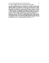
Continuous measurement data should be graphed as a dot diagramwhen the data set is small say, fewer than 20 or 25 observations. Larger data sets are summarized by grouping the observations in class intervals, preferably of equal lengths. Tài liệu giúp bạn tham khảo, ôn tập và đạt kết quả cao. Mời đọc đón xem!
Môn: Xác suất thống kê (FTU) 355 tài liệu
Trường: Trường Đại học Ngoại Thương 1.1 K tài liệu
Tác giả:


Preview text:
Revision for Mid-term Test A. Knowledge Revision
Chapter 2: Organization and Description of Data
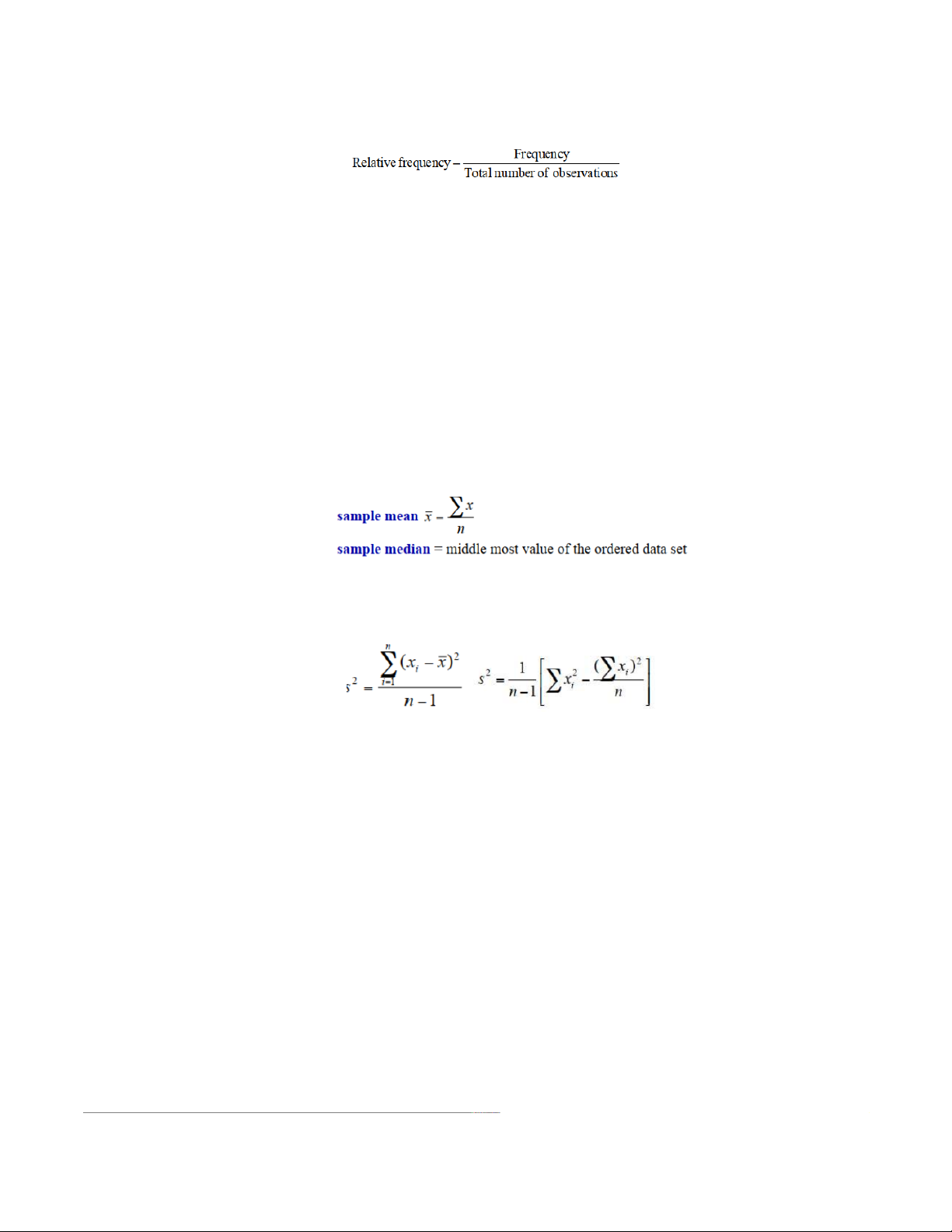
-Qualitative data refer to frequency counts in categories. These are summarized by calculating the formula:
-Data obtained as measurements on a numerical scale are either discrete or continuous.
-A discrete data set is summarized by a frequency distribution that lists the distinct data points and the
corresponding relative frequencies. Either a line diagram or a histogram can be used for a graphical display.
-Continuous measurement data should be graphed as a dot diagram when the data set is small say, fewer
than 20 or 25 observations. Larger data sets are summarized by grouping the observations in class
intervals, preferably of equal lengths. A list of the class intervals along with the corresponding relative
frequencies provides a frequency distribution, which can be graphically displayed as a histogram.
-A stem-and-leaf display is another effective means of display when the data set is not too large. It is
more informative than a histogram because it retains the individual observations in each class interval
instead of lumping them into a frequency count -
Pareto diagrams display events according to their frequency in order to highlight the most important few that occur most of the time.
-A summary of measurement data (discrete or continuous) should also include numerical measures of center and spread.
-Two important measures of center are
-The quartiles and, more generally, percentiles are other useful locators of the distribution of a data set. The
second quartile is the same as the median.
-The amount of variation or spread of a data set is measured by the sample standard deviation s. The sample variance s2 is given by
-The standard deviation indicates the amount of spread of the data points around the
mean x . If the histogram appears symmetric and bell-shaped, then the interval
includes approximately 68% of the data x ± s
includes approximately 95% of the data x ± s 2
includes approximately 99.7% of the x ± s 3 data
-Two other measures of variation are
sample range = largest observation - smallest observation
sample interquartile range = third quartile - first quartile
(The five quantities, namely, the median, the first and third quartiles, the smallest
observation, and the largest observation, together serve as useful indicators of the
distribution of a data set. These are displayed in a boxplot.)
Chapter 3: Descriptive Study of Bivariate Data -
Cross-classified data can be described by calculating the relative frequencies. -
The correlation coefficient r measures how closely the scatter approximates a straight-line pattern. -
A positive value of correlation indicates a tendency of large values of to occur with lar x ge values of y,
and also for small values of both to occur together. -
A negative value of correlation indicates a tendency of large values of to occur with small values of x y and vice versa. -
A high correlation does not necessarily imply a causal relation. -
A least squares fit of a straight line helps describe the relation of the response to the input variable y . x -
A y-value may be predicted for a known x-value by reading from the fitted line Chapter 4: Probability -
The probability model of an experiment is described by
1. The sample space, a list or statement of all possible distinct outcomes.
2. Assignment of probabilities to all the elementary outcomes. P(e) ≥ 0 and ∑ P(e) = 1. -
The probability of an event A is the sum of the probabilities of all the elementary outcomes that are in A. -
A uniform probability model holds when all the elementary outcomes is S are equiprobable. With a uniform probability model
-P(A), viewed as the long-run relative frequency of A, can be approximately determined by repeating
the experiment a large number of times.
The three basic laws of probability are: -
These are useful in probability calculations when events are formed with the operations of
complement, union, and intersection. -
The concept of conditional probability is useful to determine how the probability of
an event A must be revised when another event B has occurred. It forms the basis of the
multiplication law of probability and the notion of independence of events.
Conditional probability of A given B -
The notion of random sampling is formalized by requiring that all possible samples are equally likely
to be selected. The rule of combinations facilitates the calculation of probabilities in the context of
random sampling from N distinct units.
Chapter 5: Probability Distribution -
The outcomes of an experiment are quantified by assigning each of them a numerical
value related to a characteristic of interest. The rule for assigning the numerical value is called a random variable X. -
The probability distribution of X describes the manner in which probability is distributed over the
possible values of X. Specifically, it is a list or formula giving the pairs x and f(x) = P[X = x]. -
A probability distribution serves as a model for explaining variation in a population . -
A probability distribution has a
mean µ = ∑ (value x probability) = ∑ xi f(xi) which is interpreted as the population mean.
This quantity is also called the expected value E(X). Although X is a variable, E(X) is a constant. -
The binomial distribution with n trials and success probability p has Mean = np Variance = npq sd = npq (Recall: q = 1 – ) p - The population
variance is σ2 = E(X - µ)2 =∑(x - µ)2 f (x)
- The standard deviation σ is its square root.
- The standard deviation is a measure of the spread or variation of the population.
- Bernoulli trials are defined by the characteristics: (l) two possible outcomes, success (S) or failure (F)
for each trial; (2) a constant probability of success; and (3) independence of trials.
Sampling from a finite population without replacement violates the requirement of independence.
If the population is large and the sample size small, the trials can be treated as independent for all practical purposes.
The number of successes X, in a fixed number of Bernoulli trials, is called a binomial random
variable. Its probability distribution, called the binomial distribution, is given by where = number of trials, n
p = the probability of success in each trial, and = 1 - q p. The binomial distribution has Mean = np Standard derivation =
-A p chart displays sample proportions to reveal trends or changes in the population proportion over time. Chapter 6: Normal Distribution
-The probability distribution for a continuous random variable X is specified by a probability density curve.
-The probability that X lies in an interval from a to is determined by the a b rea under the
probability density curve between a and .
b The total area under the curve is 1 and the curve is never negative.
-The normal distribution has a symmetric bell-shaped curve centered at the mean.
-The intervals of one, two, and three standard deviations around the mean contain the
probabilities 0.683, 0.954, and 0.997, respectively.
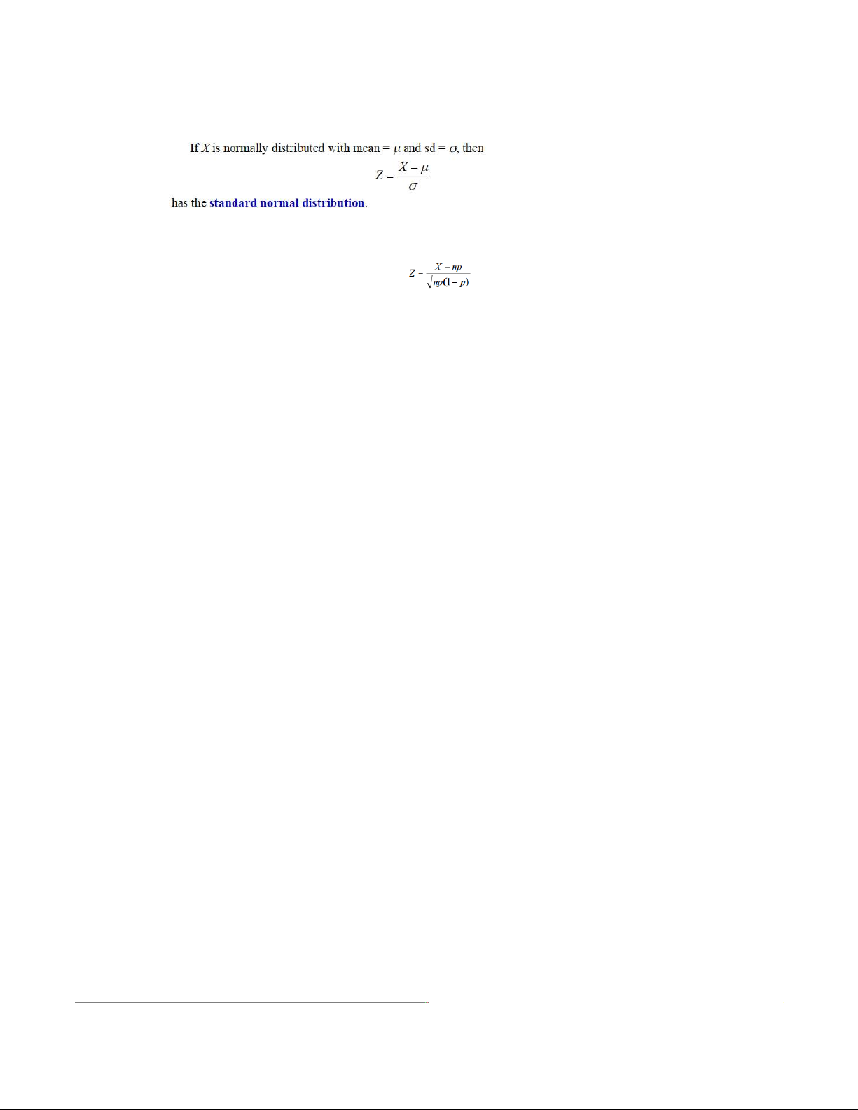
- When the number of trials is lar n
ge and the success probability is not too near 0 or p
1, the binomial distribution is well approximated by a normal distribution with mean m = and sd = . Specific np
ally the probabilities for a binomial variable X can be
approximately calculated by treating as standard normal
-The normal-scores plot of a data set provides a diagnostic check for possible
departure from a normal distribution.
Transformation of the measurement scale often helps to convert a long-tailed
distribution to one that resembles a normal distribution.
Chapter 7: Sampling Distribution
-A parameter is a numerical characteristic of the population. It is a constant although
its value is typically unknown to us. The object of a statistical analysis of sample data is to learn about the parameter.
-A numerical characteristic of a sample is called a statistic. The value of a statistic varies in repeated sampling.
-Random sampling from a population refers to independent selections where each
observation has the same distribution as the population.
-When random sampling from a population, a statistic is a random variable. The
probability distribution of a statistic is called its sampling distribution. _
-The sampling distribution of X has mean µ and standard deviation /
- , where µ = population mean, = population standard deviation, and = sample size. n
With increasing , the distribution of n
X is more concentrated around µ.
-If the population distribution is normal N(µ , ), the distribution of X is N(µ, / ).
-Regardless of the shape of the population distribution, the distribution of X is
approximately N(µ, / ), provided that is lar n
ge. This result is called the central limit theorem. B. Exercises Exercise 1.
To investigate the economic impact of doing business with the state, a sample was
taken of 15 small firms in the service sector that are vendors to the state. The data, on
the percent of total sales due to sales to the state, are
27.0, 12,0, 15.0, 1.0, 0.1, 1.0, 5.0, 0.1
8.0, 5.0, 1.0, 1.0, 3.0, 3.0, 7.0
(a) Find the sample median, first quartile, and third quartile.
(b) Find the sample 90th percentile. Exercise 2.
Loss of calcium is a serious problem for older women. At the beginning of a study
on the influence of exercise on the rate of loss, the amounts of bone mineral content in
the radius bone of the dominant hand of seven elderly women were
0.90, 1.06, 0.79, 0.85, 0.91, 0.96 Calculate (a) The sample variance
(b) The sample standard deviation Exercise 3.
The data below were obtained from a detailed record of purchases toothpaste over
several years (courtesy of A. Banerjee). The usage times (in weeks) per ounce of toothpaste for a household taken from a consumer panel were:
0.74 0.45 0.80 0.95 0.84 0.82 0.78 0.82 0.89 0.75 0.76 0.81
0.85 0.75 0.89 0.76 0.89 0.99 0.71 0.77 0.55 0.85 0.77 0.87
(a) Plot a dot diagram of the data.
(b) Find the relative frequency of the usage times that do not exceed 0.80.
(c) Calculate the mean and the standard deviation.
(d) Calculate the median and the quartiles. Exercise 4.
The following summary statistics were obtained from a data set. _x (mean) = 80.5 median = 84.0 s = 10.5 Q1 = 75.5 Q3 = 96.0
Approximately what proportion of the observations are (a) Below 96.0? (b) Above 84.0?
(c) In the interval 59.5-101.5? (d) In the interval 75.5-96.0?
(e) In the interval 49.0-112.0?
State which of your answers are based on the assumption of a bell-shaped distribution. Exercise 5.
The aging of commercial aircraft can make them more vulnerable to “skin-cracking” rivets. A major
manufacturer collected data on its three most popular models in active use to determine the magnitude of the problem.
Number of Aircraft Still in Service Model ≤ 20 Years >20 Years B7 90 123 B27 1214 435 B37 1042 9
Compare the aging of three types of planes by calculating the relative frequencies.
Exercise 6. A car dealer’s recent records on 60 sales provided the following frequency information. Engine Transmission Manual Automatic Diesel 8 12 Gas 10 30
(a) Determine the marginal totals.
(b) Obtain the table of relative frequencies.
(c) Calculate the relative frequencies separately for each row.
(d) Does there appear to be a difference in the choice of transmission between diesel and gasoline engine purchases?
Exercise 7. The tar yield of cigarettes is often assayed by the following method: A motorized smoking machine
takes a two-second puff once every minute until a fixed butt length remains. The total tar yield is determined by
laboratory analysis of the pool of smoke taken by the machine. Of course, the process is repeated on several
cigarettes of a brand to determine the average tar yield. Given here are the data of average tar yield and the
average number of puffs for six brands of filter cigarettes. Average tar
(milligrams) 12.2 14.3 15.7 12.6 13.5 14.0 Average no. of puffs 8.5 9.9 10.7 9.0 9.3 9.5 (a) Plot the scatter diagram. (b) Calculate r.
(Remark: Fewer puffs taken by the smoking machine mean a faster burn time. The
amount of tar inhaled by a human smoker depends largely on how often the smoker puffs.)
Exercise 8. The accompanying Venn diagram shows three events A, B, and C and also the probabilities of the
various intersections. (For instance, P(AB) = 0.07, P(A B ) = 0.13). Determine: (a) P(A) (b) P( BC ) (c) P( A∪ B )
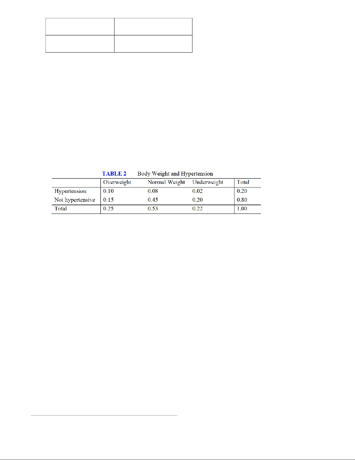
Exercise 9. A group of executives is classified according to the status of body weight and incidence
of hypertension. The proportions in the various categories appear in Table 2.
(a) What is the probability that a person selected at random from this group will have hypertension?
(b) A person, selected at random from this group, is found to be over-weight. What is the probability that this person is also hypertensive? Exercise 10.
Refer to the box “How Long Will a Baby Live?” in Section 3.2. It shows the probabilities of
death within 10-year age groups.
(a) What is the probability that a newborn child will survive beyond age 90?
(b) What is the probability that a person who has just turned 80 will survive beyond age 90? Exercise 11.
A list of important customers contains 25 names. Among them, 20 persons have their
accounts in good standing while 5 are delinquent. Two persons will be
selected at random form this list and the status of their accounts checked. Calculate the probability that
(a) Both accounts are delinquent.
(b) One account is delinquent and the other is in good standing. Exercise 12.
Describe the sample space for each of the following experiments.
(a) The record of your football team after its first game next season.
(b) The number of students out of 20 who will pass beginning swimming and graduate to the intermediate class.
(c) In an unemployment survey, 1000 persons will be asked to answer “yes” or “no” to the question “Are you
employed?” Only the number answering “no” will be recorded.
(d) A geophysicist wants to determine the natural gas reserve in a particular area. The volume will be given in cubic feet. Exercise 13.
Identify these events in the corresponding parts of Exercise 4.1. (a) Don’t lose
(b) At least half the students pass
(c) Less than or equal to 5.5% unemployment
(d) Between 1 and 2 million cubic feet Exercise 14.
Examine each of these probability assignments and state what makes it improper.
(a) Concerning tomorrow’s weather,
P(rain) = .2, P(cloudy but no rain) = .4, P(sunny) = .6
(b) Concerning your passing the statistics course, P(pass) = 2, P(fail) = .2
(c) Concerning your grades in statistics and economics courses,
P(A in statistics) = .5, P(A in economics) = .8
P(A’s in both statistics and economics) = .6 Exercise 15.
A letter is chosen at random from the word “STATISTICIAN.”
(a) What is the probability that it is a vowel?
(b) What is the probability that it is a T? Exercise 16.
A three-digit number is formed by arranging the digits 1, 5, and 6 in a random order. (a) List the sample space.
(b) Find the probability of getting a number larger than 400.
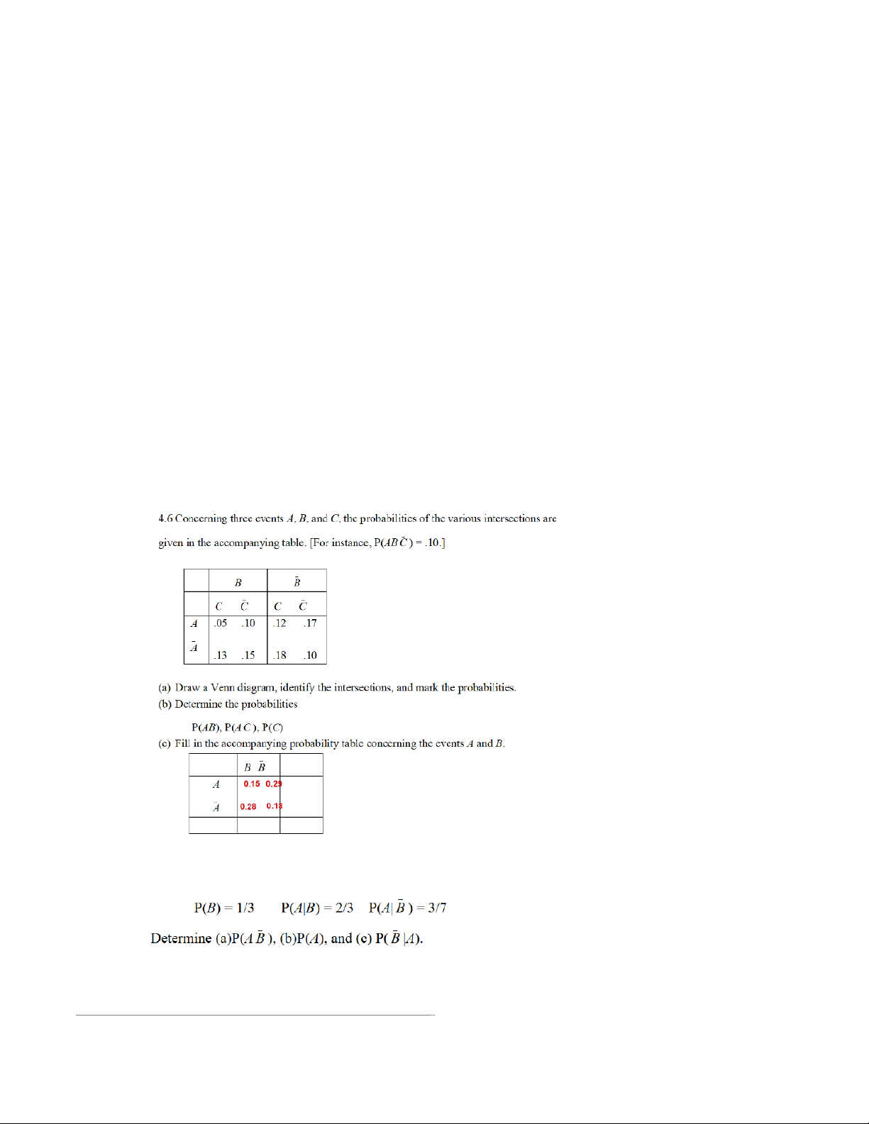
(c) What is the probability that an even number is obtained? Exercise 17. Concern… Exercise 18.
Concerning the events A and B, the following probabilities are given. Exercise 19.
Refer to the probability given in Exercise 4.6 concerning three events A, B, and C.
(a) Find the conditional probability of A given that B does not occur.
(b) Find the conditional probability of B given that both A and C occur.
(c) Determine whether or not the events A and C are independent. Exercise 20.
Three production lines contribute to the total pool of a company’s product. Line 1 provides
20% to the pool and 15% of its products are defective; Line 2 provides 50% to the pool and 5% of its products
are defective; Line 3 contributes 30% to the pool and 6% of its products are defective.
(a) What percent of the items in the pool are defective?
(b) Suppose an item is randomly selected from the pool and found to be defective. What
is the probability that it came from Line 1? Exercise 21.
Polya’s urn scheme. An urn contains 4 red and 6 green balls. One ball is drawn at random and
its color is observed. The ball is then returned to the urn, and 3 new balls of the same color are added to the
urn. A second ball is then randomly drawn from the urn that now contains 13 balls.
(a) List all outcomes of this experiment (use symbols such as R1G2 to denote the outcome of the first ball red and the second green).
(b) What is the probability that the first ball drawn in green?
(c) What is the conditional probability of getting a red ball in the second draw given that a green ball appears in the first?
(d) What is the (unconditional) probability of getting a green ball in the second draw? Exercise 22.
Suppose 30% of the trees in a forest are infested with a parasite. Four trees are randomly
sampled. Let X denote the number of the trees sampled that have the parasite. Obtain the
probability distribution of X and plot the probability histogram. Exercise 23.
The random variable X represents the number of infested trees among a random sample of n =
4 trees from the forest. Instead of the numerical value 0.3, we now denote the population proportion of infested trees by the symbol .
p Furthermore, we relabel the outcome “infested” as a success (S) and “not
infested” as a failure (F). The elementary outcomes of sampling 4 trees, the associated probabilities, and the
value of X are listed as follows. Exercise 24.
Let X denote the difference (no. of heads – no. of tails) in three tosses of a a coin.
(a) List the possible values of X.
(b) List the elementary outcomes associated with each value of X. Exercise 25.
Suppose there are two boxes. Box 1 contains 20 articles, of which 6 are defective,
and Box 2 contains 30 articles, of which 5 are defective. One article is randomly
selected from each box, and the selections from two boxes are independent. Let X denote the
total number of defective articles obtained.
(a)List the possible values of X and identify the elementary outcomes associated with each value.
(b)Determine the probability distribution of X. Exercise 26.
In an assortment of 11 lightbulbs, there are 4 with broken filaments. A customer
takes 3 bulbs from the assortment without inspecting the filaments. Find the probability
distribution of the number X of defective bulbs that the customer may get. Exercise 27.
For the following probability distribution (a) Calculate E(X). (b) Calculate sd(X).
(c) Draw the probability histogram and locate the mean. x f(x) 0.3 01 2 0.4 0.3 Exercise 28.
A student buys a lottery ticket for $1. For every 1000 tickets sold, two bicycles are to be given away in a drawing.
(a) What is the probability that the student will win a bicycle?
(b) If each bicycle is worth $160, determine the student’s expected gain. Exercise 29.
The number of overnight emergency calls X to the answering service of a heating
and air conditioning firm have the probabilities .05, .1, .15, .35, .20, and .15 for 0, 1,
2, 3, 4, and 5 calls, respectively.
(a) Find the probability of fewer than 3 calls. (b) Determine E(X) and sd(X). Exercise 30.
Let_X = average number of dots resulting from two tosses of a fair die. For instance,
if the faces 4 and 5 show, the corresponding value of _X is (4 + 5)/2 = 4.5. Obtain the probability distribution of_X. Exercise 31.
Is the model of Benoulli trials plausible in each of the following situations? Identify
any serious violations of the conditions.
(a) A dentist records if each tooth in the lower jaw has a cavity or has none.
(b) Persons applying for a driver’s license will be recorded as writing left- or righthanded.
(c) For each person taking a seat at a lunch counter, observe the time it takes to be served.
(d) Each day of the first week in April is recorded as being either clear or cloudy.
(e) Cars selected at random will or will not pass state safety inspection. Exercise 32.
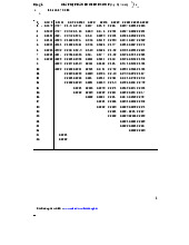
If the probability of having a male child is .5, find the probability that the third child is the first son. Exercise 33. Using the binomial table,
(a) List the probability distribution for = 5 and n = .4. p
(b) Plot the probability histogram.
(c) Calculate E(X) and Var(X) from the entries in the list from part (a).
(d) Calculate E(X) = np and Var(X) = npq and compare your answer with part (c) Exercise 34.
Given that X has the normal distribution N(60, 4), find P[55 ≤ X ≤ 63] Exercise 35.
The number of calories in a salad on the lunch menu is normally distributed with mean = 200
and sd = 5. Find the probability that the salad you select will contain (a) More than 208 calories.
(b) Between 190 and 200 calories. Exercise 36.
Let X have a binomial distribution with = 0.6 and p = 150. n
Approximate the probability that
(a) X is between 82 and 101 both inclusive. (b) X is greater than 97. Exercise 37.
For a standard normal random variable Z, find: (b) P[Z > 1.225] (a) P[Z < 1.36] (d) P[-1.37 < Z < 1.055] (c) P[0.67 < Z < 1.98] Exercise 38.
If Z is a standard normal random variable, what is the probability that (a) Z exceeds -0.72?
(b) Z lies in the interval (-1.50, 1.50)? (c) |Z| exceeds 2.0? (d) |Z| is less than 1.0? Exercise 39.
Suppose that a student’s verbal score X from next year’s Graduate Record Exam can
be considered an observation from a normal population having mean 497 and standard deviation 120. Find (a) P[X > 600]
(b) 90th percentile of the distribution
(c) Probability that the student scores below 400 Exercise 40.
It is known from past experience that 7% of the tax bills are paid late. If 20,000 tax
bills are sent out, find the probability that
(a) Less than 1350 are paid late.
(b) 1480 or more are paid late.
6.5 Because 10% of the reservation holders are “no-shows”, a U.S. airline sells 400
tickets for a flight that can accommodate 370 passengers.
(a) Find the probability that one or more reservation holders will not be accommodated on the flight.
(b) Find the probability of fewer than 350 passengers on the flight Exercise 41.
A population consists of the four numbers {0, 2, 4, 6}. Consider drawing a random sample of size 2 with replacement.
(a) List all possible samples and evaluate for each. x
(b) Determine the sampling distribution of X-.
(c) Write down the population distribution and calculate its mean µ and standard deviation σ.
(d) Calculate the mean and standard deviation of the sampling distribution of X- obtained in part (b), and
verify that these agree with µ and σ / 2 , respectively. Exercise 42.
Suppose a population distribution is normal with mean = 60 and standard deviation = 10. For a random sample of size n = 9,
(a) What are the mean and standard deviation of X- ?
(b) What is the distribution of X- ? Is this distribution exact or approximate?
(c) Find the probability that X- lies between 56 and 64. Exercise 43.
A random sample of size 150 I taken from a population that has mean = 37 and standard
deviation = 7. The population distribution is not normal.
(a) Is it reasonable to assume a normal distribution for the sample mean X ?Why and why not?
(b) Find the probability that X- lies between 36 and 38.
(c) Find the probability that X- exceeds 38.5. Exercise 44.
Suppose the amount of sun block lotion in plastic bottles laving a filling machine has
a normal distribution. The bottles are labelled 300 milliliters (ml) but the actual mean is 302 ml and the standard deviation is 2 ml.
(a) What is the probability that an individual bottle will contain less than 299 ml?
(b) If only 5% of the bottles have content that exceed a specified amount ν, what is the value of ν?
(c) Two bottles can be purchased together in a twin pack. What is the probability that the mean content of
bottles in a twin-pack is less than 299 ml? Assume the content of the two bottles are independent.
(d) If you purchase to twin-packs of the lotion, what is the probability that only one of the twin-packs has a
mean bottle content less than 299 ml?
Tài liệu liên quan:
-
Bảng giá trị phân phối thống kê poisson và student môn Xác suất thống kê| Trường Đại học Ngoại Thương
27 14 -
Bảng giá trị quyết định thống kê wilcoxon rank-sum test môn Xác suất thống kê| Trường Đại học Ngoại Thương
30 15 -
Bài 1 Định nghĩa cổ điển về xác suất môn Xác suất thống kê| Trường Đại học Ngoại Thương
26 13 -

Exercises for probability & statistics môn Xác suất thống kê| Trường Đại học Ngoại Thương
26 13 -
Đề thi cuối kỳ lý thuyết môn Xác suất thống kê| Trường Đại học Ngoại Thương
27 14