lOMoAR cPSD| 53331727
Multivariate analyses in Excel using PCA, CA and MS CAPCA Version 3.1 Torsten Madsen ©2016 Introductory comments
CAPCA is an add-in to Microsoft Excel that allows you to carry out Principal Components Analysis
(PCA), Correspondence Analysis (CA) and Metric Scaling (MS) fully integrated within Excel. The
program reads the data from your worksheets and produces additional worksheets with tables and
statistics showing the result of the analysis as well as a number of charts to illustrate it.
The background for CAPCA was a DOS based program in PACAL performing PCA and CA
analyses that I wrote in 1989 called Kvark. The program was abandoned as Erwin Scollar’s
successful program Basp and later WinBasp developed during the first half of the nineties. Both
Kvark and Basp/Winbasp, however, were hampered by tedious data input procedures and a lack of
efficient import facilities for data.
The advantage of a program for multivariate analyses within Excel appeared rather obvious, and
around 2002 I made a first attempt to create CAPCA. The program was primarily used internally at
the department, although it was disseminated to a few colleagues as well. In 2006, when I withdrew
from the university, I decided to make it generally available. It was launched as version 1, followed
in 2007 by version 2 (version 2.1 in 2010 and version 2.3 in 2012). Version 3.0 from 2014 presented
a major renewal and improvement of the user interface. The present version 3.1 features some
needed improvements to the way you can enter data for metric scaling, as well as some
improvements to the way you can present and view the results of the analyses.
CAPCA is written using the built in VBA programming language in Excel. The version of Excel
used for version 3.1 is 14 (Office 2010). I have not had the possibility to test the program using
newer versions, but it ought to work. I would appreciate if you inform me, should you encounter
difficulties running the program, if you come across regular bugs, or indeed if you have any
suggestions of improvement. The code is not password protected, and you are welcome to browse
through it and make changes if you like. Should you make regular improvements to the program, I
would appreciate if you inform me. Installing CAPCA
Installing CAPCA on your computer is simple. The only precondition is that you have Microsoft
Excel version 12 (Office 2007) or later. The program is distributed as an Excel add-in program file
(.xlam file) that is compatible with Office 2007 or later.
CAPCA Version 3.1.xlam
It is customary to place add-in files in the directory AppData/(Roaming)/Microsoft/AddIns. You will
find this as a sub-directory to the directory for your personal settings (e.g. Users/user name). The
directory may be hidden. In that case, you need to change the settings in the file browser allowing
you to see hidden directories. It is not compulsory, however, to place the file in this directory. You
may in fact place it wherever you want, but Excel will always look first for an addinn file in the above mentioned directory.
The procedure for installing in Office 2010 is the following (it differs slightly from office 2007):
If you already have CAPCA installed you should remove the add-inn file (e.g. lOMoAR cPSD| 53331727
CAPCAversion3.03.xlam) before you open Excel. When you open Excel, it will inform you that the
file is missing. Next, you activate the “Files” page in Excel and select settings. In the menu that
appear you select Add-Ins, and in the subsequent Add-Ins dialog box you select “Manage Excel
Add-ins” at the bottom of the form and press Go. You will see the name of the removed file
checked in the add-inn list. You un-check it and let Excel remove the reference. Finally, you press
browse to find “CAPCA Version 3.1.xlam” and activate it.
If you do not have a previous version of CAPCA installed, you go directly to the “Files” page in
Excel and select settings. In the menu that appear you select Add-Ins, and in the subsequent AddIns
dialog box you select “Manage Excel Add-ins” at the bottom of the form and press Go. You then
press browse to find “CAPCA Version 3.1.xlam” and activate it.
Potential problems installing CAPCA.
Hopefully you will not be met with problems when trying to run CAPCA, but with new versions of
Microsoft Windows and Microsoft Office they may appear. If you experience that a newly installed
program crash, please report it.
Previously, there were problems with outdated versions of a Microsoft library file named
REFEDIT.DLL. If you are using Office 2007 you will find the file in the library C:/Program files
(x86)/Microsoft Office/Office12. It should have a date of 26.02.2009. The original version of the
file for Office 2007, dated 26.10.2006, resulted in fatal run time errors.
The version of the file used here is dated 13.03.2010. It is placed in C:/Program files
(x86)/Microsoft Office/Office14. Preparing data for CAPCA
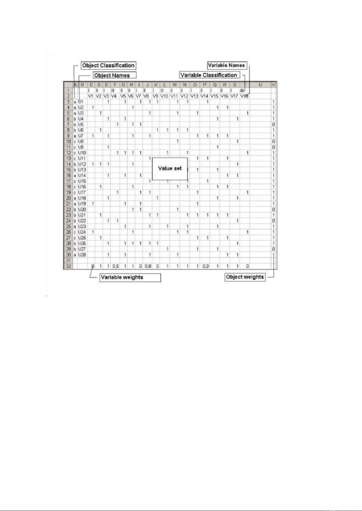
All data to be used in the analyses must be placed in an Excel worksheet. Seven sets or elements of
data are recognised: Values, Object names, Variable names, Object classes, Variable classes,
Object weights and Variable weights. Values
The set of values consist of a rectangular table of numbers, blanks or strings. In computing terms it
is a two-dimensional array (Values(i,j)), where i is the number of entries in the first dimension and j
is the number of entries in the second dimension of the array. In Excel it equals a rectangular block
of cells. Thus, if i = 28 and j = 18 it could be a block of cells with the reference C3:T30.
The type of values that you can enter into the table depends on the type of analysis. The rules
differ for a PCA, a CA and a MS analysis. In connection with the chapters, describing each of these
analyses you will find detailed information on what kind of values you can use. There is all reason
to study this information carefully, because most failures to make the program work relates to illegal values in the data set.
Object names and Variable names
Object names and Variable names consist of a row or a column of text strings. In computing terms
they are represented by one-dimensional array (ObjectNames(i) or VariableNames(j)), where i and j
are the number of entries in the arrays. In Excel it equals a horizontal or vertical stripe of cells.
Thus, if i = 28 it could be represented by a series of cells with the reference B3:B30, and if j = 18 it
could be represented by a series of cells with the reference C2:T2. 2 lOMoAR cPSD| 53331727
Each name can consist of letters or digits alone or in any combination, and there is no limitation
to the length of the names. Missing names (blank cells) are not allowed, and each name must be
unique within the set of names. Both Object names and Variable names are mandatory data.
Object classes and Variable classes
Object classes and Variable classes consist of a row or a column of text strings. In computing terms
they are represented by one-dimensional array (ObjectClasses(i) or VariableClasses(j)), where i and
j are the number of entries in the arrays. In Excel it equals a horizontal or vertical stripe of cells.
Thus, if i = 28 it could be represented by a series of cells with the reference A3:A30 and if j = 18 it
could be represented by a series of cells with the reference C1:T1
Each class name can consist of letters or digits alone or in any combination, and there is no
limitation to the length of the class names. Missing names (blank cells) are not allowed. There is no
limit to the number of different class names in the sets of object or variable classes. All class names
could be unique or they could be identical, but of course it is only meaningful with a number of
different class names somewhere in between. Object and variable classes are optional data.
Object weights and Variable weights
Object weights and Variable weights consist of a row or column of numbers. In computing terms it
is a one-dimensional array (ObjectWeights(i) or VariableWeights(j)), where i and j are the number
of entries in the arrays. In Excel it equals a horizontal or vertical stripe of cells. Thus, if i = 28 it
could be represented by a series of cells with the reference V3:V30 and if j = 18 it could be
represented by a series of cells with the reference C32:T32.
Each weight must be either 0 or 1, but for some analyses it can also be a digit between these two
values. The weights are used differently in PCA CA and MS. For information about how they may
be used you are referred to the description in connection with the individual analyses. Object
weights and Variable weights are optional. 3 lOMoAR cPSD| 53331727
Figure 1. For good practice, use a standardised layout of data for entry into CAPCA.
Organising the worksheet
Although you can place the elements of data wherever you want in a worksheet or indeed in
different worksheets if you wish, it is customary and good practice with an organised setup as the
one shown in Fig. 1. Here, object names and object classes to the left and variable names and
variable classes above flank the values. Further, object weights are placed to the right of the values
and variable weights below them.
It is not mandatory to have objects in the rows and variables in the columns of the value set, but
it is certainly good practice. It is imperative, however, that the program knows the orientation of the
value set, so if you have objects in the columns and variables in the rows you must remember to
change the default setting in the data entry page of the main form. Entering data into CAPCA
CAPCA has one main form and one auxiliary popup form. The main form has five pages: a data
entry page, a page for running CA, a page for running PCA, a page for running MS, and a page for
displaying graphics. Each page, I discussed in separate chapters. 4 lOMoAR cPSD| 53331727
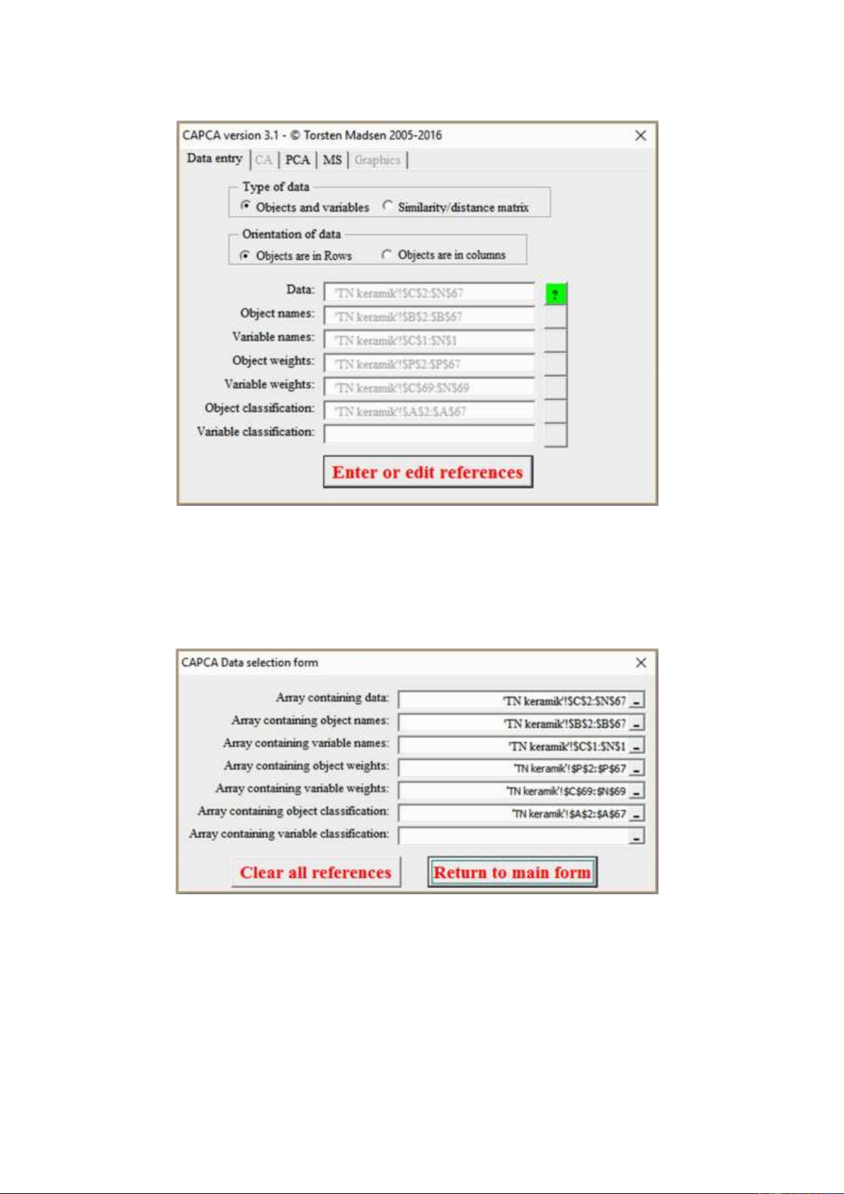
Figure 2. CAPCA main form, data entry page.
The first time you open CAPCA in a workbook, the reference controls will be blank, but as soon as
you have entered references, these will be remembered, and whenever you open CAPCA again in
that particular workbook the reference controls are filled in with the last used references (Fig. 2).
Figure 3. CAPCA data selection form.
Recording of references does not take place in the main form, but through an auxiliary popup form
opened by pressing the button “Enter or edit references” (Fig. 3).
The popup form has seven controls through which you can enter references for the seven types of
data categories. To enter a reference you either place the cursor in the reference field (mark the
existing reference if there is one), and then mark up the relevant area of data in the sheet, or you 5 lOMoAR cPSD| 53331727
click on the small square box to the left of reference. Doing this will make the popup form disappear
leaving the one control in use visible only (Fig. 4). This makes it easier to see the data in the sheet
and mark them. When done you click the small rectangular box again, and the form will reappear.
If you choose to fill in references in the controls manually, you must remember to enter the sheet
name as part of the reference. In contrast to previous versions of CAPCA, references without a sheet name are not allowed.
Figure 4. RefEdit control during reference recording.
When you press “Return to main form” the references are transferred to the main form and the popup form disappears.
You may well wonder why the reference recording is done through an auxiliary form and not
directly from the main form. The reason is that the RefEdit control does not work when embedded
in a multipage form. It summarily and ungracefully crashes the program when activated. It is not
mentioned in the documentation of the control, but a few references to this behaviour can be found on the web.
Option controls on the data entry page
There are two option controls on the data entry page. The first sets the type of data, the second sets
the orientation of data.
Type of data here refers to data as a table of objects described through variables versus data as a
table of coefficients describing the interrelationship between objects. The first is the default, and
probably the only you will ever user. Similarity coefficients are used for MS only, and even here
most users will probably choose to enter data as objects and variables and let CAPCA worry about
the calculation of similarity coefficients.
Orientation of data refers to whether objects are in rows (and variables in columns) or objects
are in columns (and variables in rows). The first is the default, and you are urged to keep this
convention. If your objects are in columns the data set will be transposed before analysis, and
eventually you will find that in all tabular output of data the objects have ended up in the rows. If
you have chosen similarity coefficients as type of data the orientation of data option will be disabled as it is irrelevant. Validation of data
A validation process is carried out continuously, triggered by almost any action in the main form.
The aim of the process is to ensure that the referenced data are suitable for analyses and to
determine what limitations there might be on these analyses. The result of the validation process is
fed back to the main form, where you can access it through the information buttons that are placed
to the right of the reference fields.
The information buttons has three states of appearance: neutral, green or red. A neutral button
has the same colour as the background of the form, and nothing will happen if you press it. A green
button or a red button will display a message box if you press it. The message box will display
information related to the data referenced in the adjoining reference field.
A green button indicates that data with some restrictions can be analysed. Thus, in fig. 2 you can
see that despite a green button and no red buttons the page for performing CA has been disabled. 6 lOMoAR cPSD| 53331727
Pressing the green button, you would find out why CA is not available.
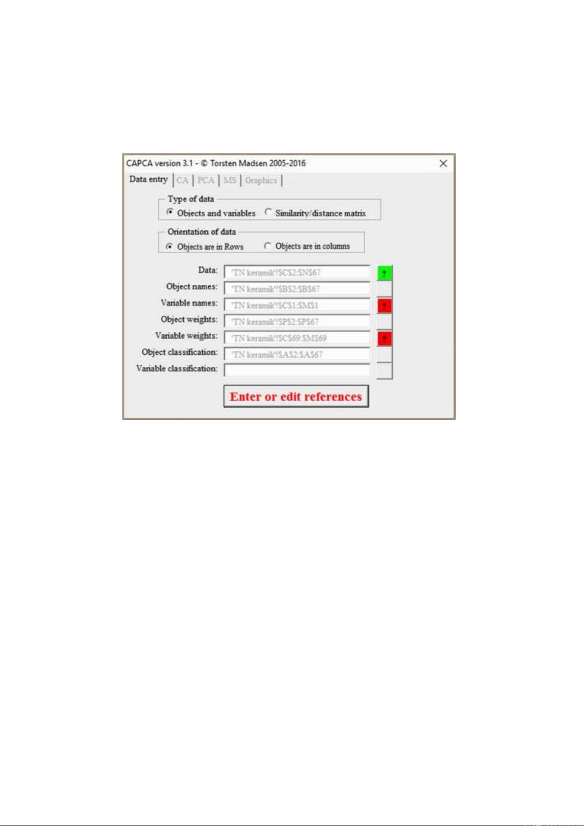
A red button indicates that something in the data referenced hinders any analysis. In Fig. 5 there
are two red buttons each triggered independently by invalid data blocking an analysis. Pressing the
buttons you will find information that explains what the problems are.
Figure 5. CAPCA main form, data entry page. Red info buttons signals invalid data. All pages other than the
data entry page has been disabled.
The following list gives an overview of the messages you can encounter in connection with the various data sets: Value set ●
You must supply a complete reference, including the sheet name - eg. Sheet!cells. ●
The data set contain 38 objects and 18 Variables. ●
The data set contain blanks. Blanks can be used in CA only. The blanks will automatically be substituted by zeroes. ●
The data set contain values that are not integers. The data cannot be used for CA analysis. ●
The data set contain values that are negative. The data cannot be used for CA analysis. ●
Log transformations in PCA are not available for variables with negative data. You may use
ArcSin transformation in stead. ●
The data set contains sums across object values that are zero. If you use a CA analysis these
objects will be eliminated from the analysis. ●
The data set contains sums across variable values that are zero. If you use a CA analysis these
variables will be eliminated from the analysis. ●
The data set contains non numeric data. It cannot be used for PCA or CA. in MS
A separate set of messages apply to similarity coefficient matrices ●
The data set contains question marks indicating missing values useable only for MS. 7 lOMoAR cPSD| 53331727 ●
The object weights supplied are ignored as data consist of similarity coefficients. ●
The variable weights supplied are ignored as data consist of similarity coefficients. ●
The variable classes supplied are ignored as data consist of similarity coefficients. ●
The data set contains variables with a mix of numeric and non-numeric data. It is not allowed in MS. ●
The similarity matrix contains non-numeric data. It cannot be analysed. ●
Data appears to constitute a similarity or distance matrix. Please check the appropriate option. ●
It is not a symmetric matrix. It cannot be used as a similarity coefficient matrix. ●
Data contain negative data. Only positive values are allowed in a similarity coefficient matrix. ●
The diagonal values are not identical. They must be in a similarity coefficient matrix. ●
Off-diagonal values are larger than the diagonal values. They cannot be in a similarity coefficient matrix. ●
Values are not mirrored around the diagonal. They must be in a similarity coefficient matrix.
Object names and Variable names ●
You must supply a complete reference, including the sheet name - eg. Sheet!cells. ●
The reference to object names must be one-dimensional. Names must be in one row or one column exclusively. ●
The reference to variable names must be one-dimensional. Names must be in one row or one column exclusively. ●
There are ## objects in your dataset and ## object names in the names array. The number must be the same. ●
There are ## variable in your dataset and ## variable names in the names array. The number must be the same. ●
One or more names are blank. A name must contain letters and or numbers. ●
There are duplicate names. All names must be unique. The following are duplicates: ●
You must provide names for the objects to run an analysis. ●
You must provide names for the variables to run an analysis.
Object classes and Variable classes ●
You must supply a complete reference, including the sheet name - eg. Sheet!cells. ●
You must provide names for the objects to run an analysis. ●
You must provide names for the variables to run an analysis. ●
The reference to object classes must be one-dimensional. Classes must be in one row or one column exclusively. ●
The reference to variable classes must be one-dimensional. Classes must be in one row or one column exclusively. ●
There are ## objects in your dataset and ## object classes in the class array. The number must be the same. ●
There are ## variables in your dataset and ## variable classes in the class array. The number must be the same. ●
One or more class names are blank. A class name must contain letters and or numbers.
Object Weights and Variable weights ●
You must supply a complete reference, including the sheet name - eg. Sheet!cells. ●
The reference to object weights must be one-dimensional. Weights must be in one row or one column exclusively. 8 lOMoAR cPSD| 53331727 ●
The reference to variablet weights must be one-dimensional. Weights must be in one row or one column exclusively. ●
There are ## objects in your dataset and ## weights in the weights array. The number must be the same. ●
There are ## variables in your dataset and ## weights in the weights array. The number must be the same. ●
Weights are found that contain blanks or non digit values. All values must be digits. ●
Some weights are either larger than 1 or smaller than 0. All values must be between 1 and 0. ●
In connection with MS only weights of 1 or 0 are valid. All other values will be converted to 1. 9 lOMoAR cPSD| 53331727
Calculating eigenvectors – number and precision
All three types of analyses in CAPCA are based on finding the eigenvectors (principal components
or principal axes) of a matrix of values. You provide the values – the data, but depending on which
type of analysis you select – CA, PCA or MS, certain changes are made to data prior to analysis.
The actual calculations – the Eigen-decomposition, or in a broader sense the single value
decomposition – are, however, the same for all three types of analyses. The calculation of
Eigenvectors in CAPCA is based on an iterative algorithm published by Wright (1985).
You can calculate as many eigenvectors as the smallest dimension of your data. If there are fewer
variables than objects the maximum number equals the number of variables. If there are fewer
objects than variables the maximum number equals the number of objects. The default number of
eigenvectors calculated is 3, but you can set any number for each of the three types of analysis. If
you enter a number higher than the highest possible it is reduced to that number. If you enter a
number smaller than the lowest possible (2) it is altered to the default number 3. The same applies if
what you write cannot be interpreted as a number. Changing the number of eigenvectors to be
calculated is done in the main control form on the individual pages for CA, PCA and MS.
It is not possible, at least not for larger matrices, to calculate the eigenvectors directly, simply
because there are too many unknown variables in the equation. Therefore, general algorithms to find
eigenvectors and corresponding eigenvalues are iterative. An iterative method for calculating
eigenvectors and eigenvalues typically works through a sequence of guesses on appropriate
eigenvectors and eigenvalues. After each guess it is checked how close the suggested values come
to solve the equation. The result is used to correct the next guess in a direction that will give an even
better fit. To control the sequence of guesses a convergence value is calculated that continuously
monitor how close to a perfect fit the guesses are. When the convergence value has become
sufficiently small and has reached a preset stop value the iterative process terminates.
The iterative method is not meant to, and indeed cannot find the true eigenvectors and
eigenvalues. The result is always an approximation, and if we set our stop value too small we may
occasionally experience that the iteration cannot find a satisfactory approximation. Therefore, it is
necessary to have an alternative way to stop the iteration. In CAPCA this is done by stopping the
iterative process if it exceeds 1000 loops.
It is important to note that the growing stability in the calculation of eigenvectors and
eigenvalues expressed through the falling convergence value does not happen equally across all
calculated eigenvectors. In general, stability is reached progressively through the sequence of
eigenvectors/principal axes, and indeed it is questionable if stability can ever be reached for the last
eigenvectors in a large value set.
This implies that if you are interested in the first two-three eigenvectors/principal axes only, you
need not have a very small stop value. If, on the other hand, you want to have all eigenvectors
calculated you need to set a small stop value. In CAPCA you control the precision through an option
box with the choice of low, medium or high precision, where medium is the default setting.
An example can illustrate the influence of these three settings.
93 objects with 41 were analysed using a CA with 20 eigenvectors/principal axes required. With
low precision the analysis took 264 iterations to converge. With medium precision the number was
320 and with high precision it was 451. If we compare the eigenvectors and eigenvalues calculated
with the three precisions we find that with low precision compared to high precision there is no
deviation for the first 8 eigenvectors, while for the last 12 there is an irregular pattern of deviation
up to 0.000005. If we compare medium precision to high precision there is no deviation for the first
12 eigenvectors, while for the last 8 there is an irregular pattern of deviation up to 0.000001. 10 lOMoAR cPSD| 53331727 Running a PCA
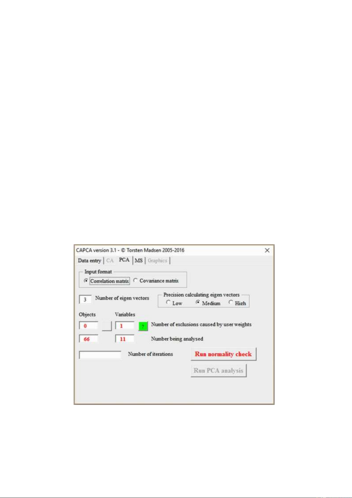
Fig. 6 shows the PCA page of the main control form. This page is enabled if the validation of data
has shown that a PCA can be run with the data provided. Otherwise it will be disabled. The page
provides an option box for setting the input format – whether data should be analysed through
correlations coefficients or covariance coefficients (se below). Further, the page contain controls for
setting the number of eigenvectors to be calculated and the precision with which they should be
calculated (se the chapter on Calculating eigenvectors – number and precision). The following two
check boxes controls if weights for objects and variables should be applied. They are only enabled if
you have provided weights, and you must actively check them to apply the weights you have
supplied. The following four info-fields inform you on how many objects and variables are being
analysed and how many (if any) objects and variables have been excluded by user weights (see
below). If exclusions occur a green button next to the number becomes available. Pressing this will
open a message box giving the names of the objects and/or variables excluded. Finally, when the
analysis has been completed, the number of iterations will be displayed.
Acceptable values for PCA analysis
All values in the provided data set must be numbers. They can be either integers or real, negative or
positive, and include zero. Text is not allowed, and the only special characters allowed are (-) (.) and
(,). They are interpreted according to the national setup of your computer (e.g. -2.455,23 in a Danish
setup compared -2,455.23 in an English setup). Remember that Excel as a rule will align everything
it reads as a number to the right and everything else to the left. Anything you see aligned to the left
in your data in the worksheet will trigger an error.
Figure 6. The PCA page of the CAPCA control form 11 lOMoAR cPSD| 53331727
Setting the input format
You can choose whether the PCA should be based on a correlation matrix (default) or a covariance
matrix. In both cases alterations are made to the data you provide, but in different ways and with different results.
With the covariance matrix the values of a variable are altered by subtracting the mean value of
the variable and divide by the square root of the total number of values minus one. Xi (Xi X) n 1
In this way the values of a variable will be centred on its mean value, but relatively speaking, size
differences between variables are not affected. If you have a variable of length and a variable of
thickness, the sum of the values of the first will still be larger than the sum of values of the latter.
With a correlation matrix the values of a variable are altered by subtracting the mean value of the
variable and divide by the standard deviation of the variable multiplied with the square root of the
total number of values minus one. ( X i X ) n ( X i X ) 2 1 ( n 1) X n i 1
In this way the values of a variable will not only be centred on its mean value, but the magnitude of
the distribution around the centre will be altered (standardised) to unity as well. Thus all variables
will become of the same size. If you have a variable of length and a variable of thickness, the sum
of the values of the first will be the same as the sum of values of the latter.
Which one of the two methods to choose depends on the nature of your data. If your data consists
of measurements, where each variable is logically independent of other variables – typically size
measurements of artefacts – you should probably use correlation coefficients. If on the other hand
there is a logical dependence between variables you should probably use covariance coefficients.
Typically, this could be measures of composition, whether an alloy composition or an artefact
composition – but then you might well choose to use a CA in stead.
I do not believe there is a clear cut answer to what type of coefficients you should prefer in
different situations, but as in archaeology we use PCA as an explorative tool the most sensible thing
to do is probably to use both to see what creates the most meaningful results.
Using weights in a PCA
Weights used in a PCA are numbers between 0 and 1 including both. Weights can be applied to both
objects and variables. A weight of 0 implies that an object or variable should be excluded from the
analysis, while a weight of 1 implies that an object or variable should be included in the analysis. If
weights are not present all objects and variables will be included. A number between 0 and 1 is used
as a multiplication factor that changes all values of the associated object or variable.
The obvious use of weights as multiplication factors in a PCA is to remove unwanted sideeffects
of the measurements established through the variables. Take pottery for instance. If you have taken
a series of measurements of different parts of the pots to discern morphological differences, you will
soon find out that the size of the pots will be the dominating result of the analysis and not their
shape. To counter this problem you will have to get rid of the size factor. One way to do this is to
calculate the approximate volume of each pot using the measurements and then use the volumes to
establish a weight factor (largest volume/ volume of pot). Or you may simply take the most
dominating size variable – say pot height and use this to create a weight factor (largest height/
height of pot). You would then of course have to exclude pot height from the analysis. 12 lOMoAR cPSD| 53331727
Checking normality and applying transformations of variables
If you are using correlation coefficients as input, then ideally all variables should be normally
distributed. When dealing with measurement data this is seldom the case. In most cases the
distribution will be skewed towards the higher values.
One way to counter this problem is to change the scale of the variables through some form of
numerical transformation. The most common transformation to use is a logarithmic transformation.
In CAPCA transformations based on either Log(10) or Arc Sin are implemented. Log
transformations will only work with positive number. You will not be able to use transformations, if
you have chosen the covariance matrix input.
There are two buttons on the PCA page called Run normality check and Run PCA analysis. If
you are using covariance coefficients the Run PCA analysis is the only button enabled, as normality
is not an issue. If, on the other hand, correlation coefficients are used the Run normality check is the
only button enabled. As a minimum you have to produce the information on normality before you
run the analysis, even if you do not use it.
When you press Run normality check a new worksheet is added to your workbook. It is named
the same as your data worksheet with the addition normality(PCA). If the resulting name is longer
than 32 chars the first part is abbreviated (that is normality(PCA) will always be present). The first
part of the worksheet shows the data as analysed. Below this a set of summary statistics are printed
(Fig. 7). The statistics shown are: sum, mean, standard deviation, skewness and kurtosis. Skewness
and kurtosis are of main interest here.
Skewness is a measure that shows the degree of asymmetry around the mean value of a variable.
It attains zero for perfect symmetry, has a growing positive value with a growing asymmetric tail
towards higher values, and has a growing negative value with a growing asymmetric tail towards lower values.
Kurtosis is a measure that shows whether the distribution of values is higher or lower than the
normal distribution associated with the standard deviation. Positive values indicate a too high
(narrow) distribution and negative values a too low (broad) distribution. Skewness is calculated as: n x x 3 (n 1)(n 2) nj 1 j s And kurtosis as: n(n 1) jn1 xj s x 4
(n3( n2)( n1) 2 3)
(n 1)(n 2)(n 3)
where s is the standard deviation of the variable and n its number of values. For both skewness and
kurtosis the build in Excel functions are used.
Following the summary statistics is a section showing what the normality distributions will be for
each variable using either Log transformation or ArcSin transformation. Looking at the example in 13 lOMoAR cPSD| 53331727
Fig. 7 it can be seen that normality can be improved using transformations. Whether, the use of
transformations will improve the results is another matter. They will certainly change them, but
whether they become more interpretable is entirely up to you to decide. As we use PCA in an
exploratory way there are no rules saying that you must transform your data. You decide.
Figure 7. Part of the normality(PCA) sheet showing summary statistics for each variable, normality distributions
with different types of transformations, and selection boxes for choosing transformation types.
To apply a transformation you use the last section in the normality(PCA) sheet (Fig. 7). It consists
of one row of cells. In each of these are written No transform. When you activate one of these cells
a small down arrow will appear at the end of the cell. If you click this arrow a drop-down box
appears where you can select the transformation type you want (Fig. 8).
Figure 8. Selecting transformation type in the normality(PCA) sheet.
When you have activated the Run normality check button to create the normality(PCA) page the
button will be disabled and instead the Run PCA analysis will be enabled. Running the analysis
Pressing the Run PCA analysis will run a PCA of your data and subsequently add a new worksheet
to your workbook. It is named the same as your data worksheet with the addition statistics(PCA). If
the resulting name is longer than 32 chars the first part is abbreviated (that is statistics(PCA) will
always be present). The worksheet will contain the results of the analysis in tabular form.
The first section of the sheet shows the matrix of correlations coefficient used as the starting point
for calculations (Fig. 9) – or the matrix of covariance coefficients, if this was the starting point of the analysis.
For correlation coefficients (Pearson’s r) the coefficients are calculated as:
N (xi x)(yi y) r i 1 N (xi x)2 N (yi y)2 14 lOMoAR cPSD| 53331727 i 1 i 1
For covariance coefficients the coefficients are calculated as:
n (xi x)(yi y) i 1 n
Figure 9. Correlation coefficient matrix used as a starting point for the PCA.
The second section shows the Eigen values for the calculated Principal components (Fig. 10). The
eigenvalues reflects the amount of information that is associated with the individual principal
components or eigenvectors. Knowing the total score of the eigenvalues we can calculate how large
a part of the total information each component covers. Consequently, we know how large a
percentage of the total information is explained by the first, the second, etc. principal components.
Figure 10. Information on eigenvalues and explanation percentages for a PCA.
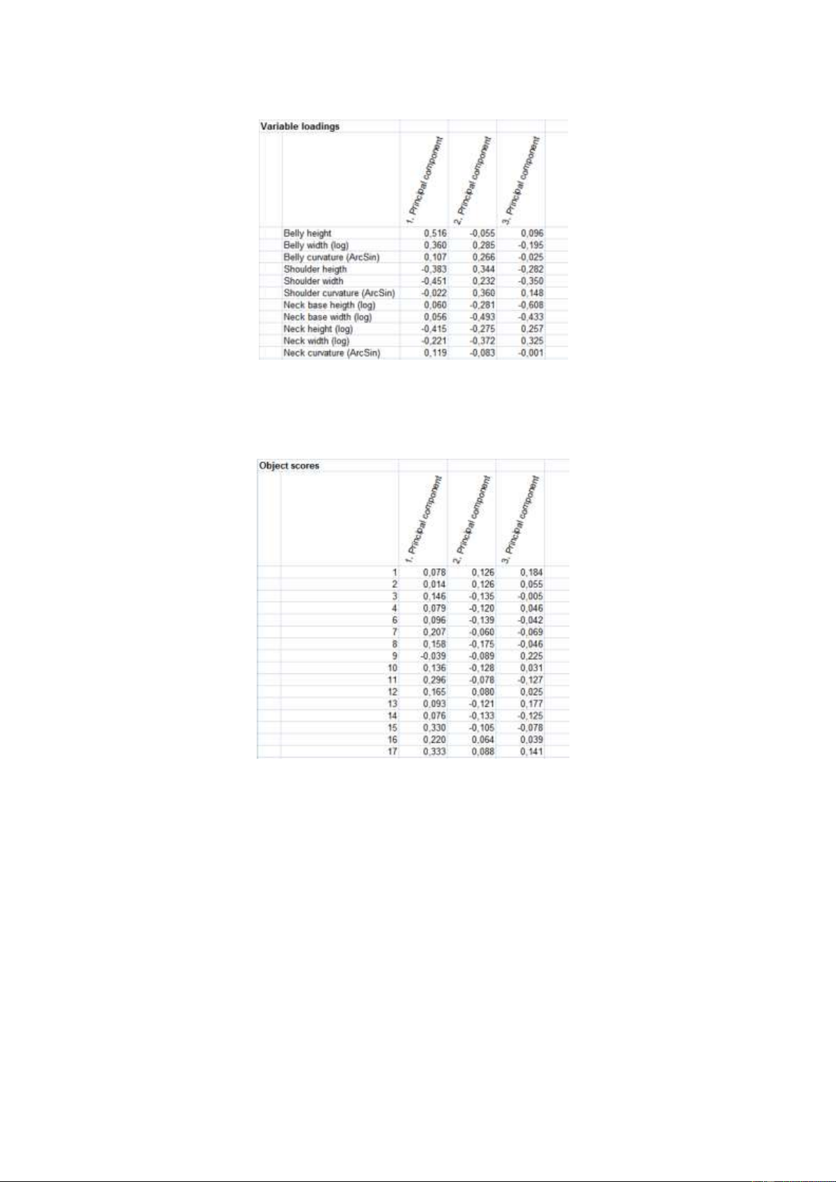
The third section shows the variable loadings (Fig. 11). That is the coordinates of the variables on
the individual principal components (axes).
If you have used transformations of the variables to obtain normality, the type of transformation
will be noted in brackets following the variable names. 15 lOMoAR cPSD| 53331727
Figure 11. Information on variable loadings for a PCA.
The fourth and final section shows object scores (Fig. 12). That is the coordinates of the objects on
the individual principal components (axes).
Figure 12. Information on object scores for a PCA. 16 lOMoAR cPSD| 53331727 Running a CA
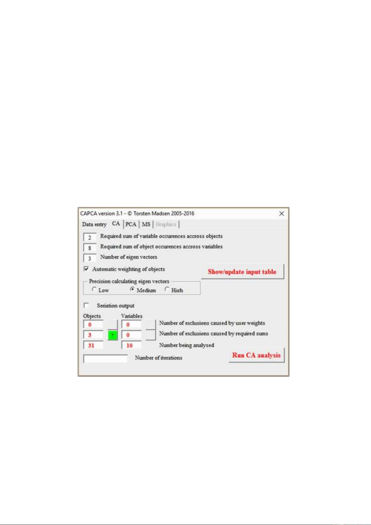
Fig. 13 shows the CA page of the main control form. This page is enabled if the validation of data
has shown that a CA can be run with the data provided. Otherwise it will be disabled. The page
provides controls for setting the number of Eigen vectors to be calculated and the precision with
which they should be calculated (se the chapter on Calculating Eigen vectors – number and
precision). When the analysis has been completed, the number of iterations will be displayed at the bottom of the form.
Values acceptable for CA analysis
All values in the dataset must be positive integers including zero. No special characters including (),
(.) and (,) are allowed, or stated differently negative values and real numbers are not allowed. For
practical reasons blank cells are allowed. They will be interpreted as zeroes and converted to such
on import. It is only in CA that blank cells are read as zeroes. In PCA they are not allowed and in
MS they are treated differently. Remember that Excel as a rule will align everything it reads as a
number to the right and everything else to the left. Anything you see aligned to the left in your data
in the worksheet will trigger an error.
Figure 13. The CA page of the CAPCA control form Using weights in a CA
The use of weights in a CA is much more complicated than in a PCA and of far greater value. First
of all, weighting is actually in use regardless of whether you have supplied weighs or not. The
reason for this is that there is a required sum of objects across variables and variables across objects
that must be observed. For computational reasons the minimum must be 1. If you supply either
objects or variables with a sum of 0 they will automatically be excluded. You can set the minimum 17 lOMoAR cPSD| 53331727
number of sums for both objects and variables in the form. The default value for both is 2. Objects
and variables with a lower sum than the one supplied will be removed.
You can also supply you own weights of course. These are numbers between 0 and 1 both
included. Weights can be applied to both objects and variables. A weight of 0 implies that the object
or the variable should be excluded from the analysis, while a weight of 1 implies that an object or
variable should be included in the analysis. A number between 0 and 1 is used as a multiplication
factor that changes all values of the associated object or variable.
Six info-fields inform you on how many objects and variables are being analysed and how many
(if any) objects and variables have been excluded by user weights and/or by required sums. If
exclusions have occurred a green button next to the number becomes available. Pressing this will
open a message box giving the names of the objects and/or variables excluded.
You should note that the user weights in combination with required sums, or indeed required
sums alone may start a chain reaction of exclusions, where further objects or variables falls for the
sums requirements as numbers dwindle because of previous exclusions.
The use of weighting (multiplication) factors between 0 and 1is closely associated with the
concept of mass and inertia of objects and variables in a CA (see below). In short the result of a CA
is heavily influenced by the absolute size (mass) of an object or a variable as well as how much they
divert in composition from the average (inertia). Both mass and inertia may result in what is known
as outliers that dominates the result and obscures the structure in the rest of the material on the first
few principal components. To lessen the effect of mass and inertia, weights are an effective tool.
There is one classical situation where mass can become a major problem. If you are analysing
settlement units based on their content of artefact types, you will almost always have a situation
where the units differ considerably with respect to number of artefacts. It can be a result of the
actual size of the units, but more often than not, it is the result of how large a part that has been
excavated. The traditional way to counter this problem in archaeology has been to calculate
percentages, but in principle percentages should only be calculated for sums above 100, and under
no circumstances below 50. To use a direct percentage calculation in a CA is therefore a bad idea, as
a CA safely can handle sums of objects and variables below 100 in this type of material. An
alternative approach is to weight objects with a sum above 100 down to this figure, but leave the
objects with a sum below 100 as they are. What the minimum sum should be in this type of study is
open to individual evaluation, but 10 seem to be a safe size and in many cases you can probably go lower.
For situations like the one outlined above I have included an option box for automatic weighting
of objects that will weight down all objects with a sum above 100 down to a sum of 100. You can
then combine this with a required sum of objects to set up a suitable analysis. For sparse matrices
like counts of types in graves or presence/absence registrations this facility is of no use of course. 18 lOMoAR cPSD| 53331727
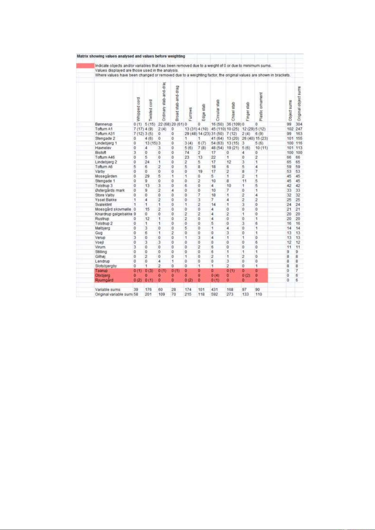
Figure 14. Table of data before and after weighting.
Viewing input data before running the CA
Because of the often complex alterations to your data following the use of weighting, it can be
useful to audit the resulting input data before you run the analysis. If you press Show/update input
data a new worksheet is added to your workbook. It is named the same as your data worksheet with
the addition tables(CA). If the resulting name is longer than 32 chars the first part is abbreviated
(that is tables(CA) will always be present).
The first part of the worksheet shows a table of the data to be analysed combined with the
original data in brackets if changes has occurred due to weighting (Fig. 14). If the weighting has
resulted in the removal of variables and/or objects these are marked out in red. Below the table, two
lines show the sum of variables after weighting and the original sums. To the right of the table two
columns show the sum of objects after weighting and the original sums.
The table in Fig. 14 shows the scenario outlined above with an automatic weighting combined
with minimum sum of objects for a number of settlement units.
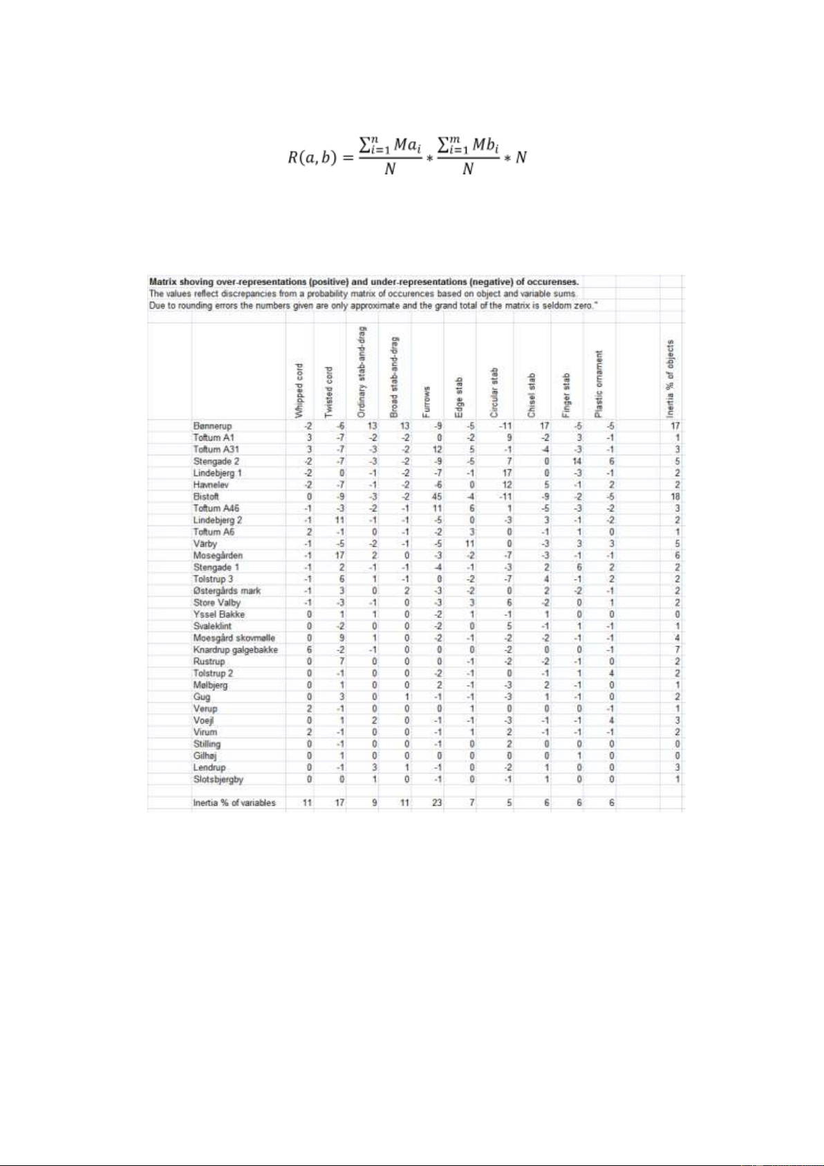
The second part of the worksheet shows a table of over- and under-representations in the dataset
under the assumption that the dataset is unstructured (Fig. 15). Unstructured is here defined as a
matrix of randomised occurrences based on the actual object and variable sums. More specifically,
if we take the sums of objects and the sums of variables as given, we can calculate a table of
occurrences as a randomisation based on these sums. This is done as follows: 19 lOMoAR cPSD| 53331727
Where R is the randomized matrix, M is the data matrix, a is a given row, b is a given column, m is
the number of rows, n is the number of columns, and N is the grand total of values in the data matrix.
Figure 15. over- and under-representations of occurrences in the data set.
What is shown (Fig. 15) is the differences between the actual values in the data matrix and the
values in the randomised matrix. This representation of data is very useful as it is the actual starting
point for a CA. It immediately gives you an impression of where the main discrepancies are
between what is and what should be expected – discrepancies that will structure the results of the analysis.
Along the margins of the table the inertia percentages are given. What is shown here is simply
how large a part of the total set of discrepancies is associated with the individual objects and with
the individual variables. The higher an inertia percentage the higher the influence of an object or a
variable on the result of the analysis becomes. 20