Probability concepts and applications: a comprehensive overview môn Xác suất thống kê| Trường Đại học Ngoại Thương

5. Probability A. Introduction B. Basic Concepts
C. Permutations and Combinations D. Poisson Distribution E. Multinomial Distribution F. Hypergeometric Distribution G. Base Rates H. Exercises
Probability is an important and complex field of study. Fortunately, only a few
basic issues in probability theory are essential for understanding statistics at the
level covered in this book. These basic issues are covered in this chapter.
The introductory section discusses the definitions of probability. This is not
as simple as it may seem. The section on basic concepts covers how to compute
probabilities in a variety of simple situations. The section on base rates discusses
an important but often-ignored factor in determining probabilities. 185
Remarks on the Concept of “Probability” by Dan Osherson Prerequisites •None Learning Objectives
1. Define symmetrical outcomes
2. Distinguish between frequentist and subjective approaches
3. Determine whether the frequentist or subjective approach is better suited for a given situation
Inferential statistics is built on the foundation of probability theory, and has been
remarkably successful in guiding opinion about the conclusions to be drawn from
data. Yet (paradoxically) the very idea of probability has been plagued by
controversy from the beginning of the subject to the present day. In this section we
provide a glimpse of the debate about the interpretation of the probability concept.
One conception of probability is drawn from the idea of symmetrical
outcomes. For example, the two possible outcomes of tossing a fair coin seem not
to be distinguishable in any way that affects which side will land up or down.
Therefore the probability of heads is taken to be 1/2, as is the probability of tails.
In general, if there are N symmetrical outcomes, the probability of any given one
of them occurring is taken to be 1/N. Thus, if a six-sided die is rolled, the
probability of any one of the six sides coming up is 1/6.
Probabilities can also be thought of in terms of relative frequencies. If we
tossed a coin millions of times, we would expect the proportion of tosses that came
up heads to be pretty close to 1/2. As the number of tosses increases, the proportion
of heads approaches 1/2. Therefore, we can say that the probability of a head is 1/2.
If it has rained in Seattle on 62% of the last 100,000 days, then the
probability of it raining tomorrow might be taken to be 0.62. This is a natural idea
but nonetheless unreasonable if we have further information relevant to whether it
will rain tomorrow. For example, if tomorrow is August 1, a day of the year on
which it seldom rains in Seattle, we should only consider the percentage of the
time it rained on August 1. But even this is not enough since the probability of rain
on the next August 1 depends on the humidity. (The chances are higher in the
presence of high humidity.) So, we should consult only the prior occurrences of 186
August 1 that had the same humidity as the next occurrence of August 1. Of
course, wind direction also affects probability. You can see that our sample of prior
cases will soon be reduced to the empty set. Anyway, past meteorological history is
misleading if the climate is changing.
For some purposes, probability is best thought of as subjective. Questions
such as “What is the probability that Ms. Garcia will defeat Mr. Smith in an
upcoming congressional election?” do not conveniently fit into either the symmetry
or frequency approaches to probability. Rather, assigning probability 0.7 (say) to
this event seems to reflect the speaker's personal opinion --- perhaps his
willingness to bet according to certain odds. Such an approach to probability,
however, seems to lose the objective content of the idea of chance; probability becomes mere opinion.
Two people might attach different probabilities to the election outcome, yet
there would be no criterion for calling one “right” and the other “wrong.” We
cannot call one of the two people right simply because she assigned higher
probability to the outcome that actually transpires. After all, you would be right to
attribute probability 1/6 to throwing a six with a fair die, and your friend who
attributes 2/3 to this event would be wrong. And you are still right (and your friend
is still wrong) even if the die ends up showing a six! The lack of objective criteria
for adjudicating claims about probabilities in the subjective perspective is an
unattractive feature of it for many scholars.
Like most work in the field, the present text adopts the frequentist approach
to probability in most cases. Moreover, almost all the probabilities we shall
encounter will be nondogmatic, that is, neither zero nor one. An event with
probability 0 has no chance of occurring; an event of probability 1 is certain to
occur. It is hard to think of any examples of interest to statistics in which the
probability is either 0 or 1. (Even the probability that the Sun will come up tomorrow is less than 1.)
The following example illustrates our attitude about probabilities. Suppose
you wish to know what the weather will be like next Saturday because you are
planning a picnic. You turn on your radio, and the weather person says, “There is a
10% chance of rain.” You decide to have the picnic outdoors and, lo and behold, it
rains. You are furious with the weather person. But was she wrong? No, she did not
say it would not rain, only that rain was unlikely. She would have been flatly
wrong only if she said that the probability is 0 and it subsequently rained. 187
However, if you kept track of her weather predictions over a long period of time
and found that it rained on 50% of the days that the weather person said the
probability was 0.10, you could say her probability assessments are wrong.
So when is it accurate to say that the probability of rain is 0.10? According
to our frequency interpretation, it means that it will rain 10% of the days on which
rain is forecast with this probability. 188 Basic Concepts by David M. Lane Prerequisites
•Chapter 5: Introduction to Probability Learning Objectives
1. Compute probability in a situation where there are equally-likely outcomes
2. Apply concepts to cards and dice
3. Compute the probability of two independent events both occurring
4. Compute the probability of either of two independent events occurring
5. Do problems that involve conditional probabilities
6. Compute the probability that in a room of N people, at least two share a birthday
7. Describe the gambler’s fallacy
Probability of a Single Event
If you roll a six-sided die, there are six possible outcomes, and each of these
outcomes is equally likely. A six is as likely to come up as a three, and likewise for
the other four sides of the die. What, then, is the probability that a one will come
up? Since there are six possible outcomes, the probability is 1/6. What is the
probability that either a one or a six will come up? The two outcomes about which
we are concerned (a one or a six coming up) are called favorable outcomes. Given
that all outcomes are equally likely, we can compute the probability of a one or a six using the formula:
 ="""
"""  "
In this case there are two favorable outcomes and six possible outcomes. So the
probability of throwing either a one or six is 1/3. Don't be misled by our use of the
term “favorable,” by the way. You should understand it in the sense of “favorable
to the event in question happening.” That event might not be favorable to your
well-being. You might be betting on a three, for example. 189
The above formula applies to many games of chance. For example, what is
the probability that a card drawn at random from a deck of playing cards will be an
ace? Since the deck has four aces, there are four favorable outcomes; since the
deck has 52 cards, there are 52 possible outcomes. The probability is therefore 4/52
= 1/13. What about the probability that the card will be a club? Since there are 13
clubs, the probability is 13/52 = 1/4.
Let's say you have a bag with 20 cherries: 14 sweet and 6 sour. If you pick a
cherry at random, what is the probability that it will be sweet? There are 20
possible cherries that could be picked, so the number of possible outcomes is 20.
Of these 20 possible outcomes, 14 are favorable (sweet), so the probability that the
cherry will be sweet is 14/20 = 7/10. There is one potential complication to this
example, however. It must be assumed that the probability of picking any of the
cherries is the same as the probability of picking any other. This wouldn't be true if
(let us imagine) the sweet cherries are smaller than the sour ones. (The sour
cherries would come to hand more readily when you sampled from the bag.) Let us
keep in mind, therefore, that when we assess probabilities in terms of the ratio of
favorable to all potential cases, we rely heavily on the assumption of equal probability for all outcomes.
Here is a more complex example. You throw 2 dice. What is the probability
that the sum of the two dice will be 6? To solve this problem, list all the possible
outcomes. There are 36 of them since each die can come up one of six ways. The
36 possibilities are shown in Table 1. 190 Table 1. 36 possible outcomes. Die 1 Die 2 Total Die 1 Die 2 Total Die 1 Die 2 Total 1 1 2 3 1 4 5 1 6 1 2 3 3 2 5 5 2 7 1 3 4 3 3 6 5 3 8 1 4 5 3 4 7 5 4 9 1 5 6 3 5 8 5 5 10 1 6 7 3 6 9 5 6 11 2 1 3 4 1 5 6 1 7 2 2 4 4 2 6 6 2 8 2 3 5 4 3 7 6 3 9 2 4 6 4 4 8 6 4 10 2 5 7 4 5 9 6 5 11 2 6 8 4 6 10 6 6 12
You can see that 5 of the 36 possibilities total 6. Therefore, the probability is 5/36.
If you know the probability of an event occurring, it is easy to compute the
probability that the event does not occur. If P(A) is the probability of Event A, then
1 - P(A) is the probability that the event does not occur. For the last example, the
probability that the total is 6 is 5/36. Therefore, the probability that the total is not 6 is 1 - 5/36 = 31/36.
Probability of Two (or more) Independent Events
Events A and B are independent events if the probability of Event B occurring is
the same whether or not Event A occurs. Let's take a simple example. A fair coin is
tossed two times. The probability that a head comes up on the second toss is 1/2
regardless of whether or not a head came up on the first toss. The two events are
(1) first toss is a head and (2) second toss is a head. So these events are
independent. Consider the two events (1) “It will rain tomorrow in Houston” and
(2) “It will rain tomorrow in Galveston” (a city near Houston). These events are
not independent because it is more likely that it will rain in Galveston on days it
rains in Houston than on days it does not. 191 Probability of A and B
When two events are independent, the probability of both occurring is the product
of the probabilities of the individual events. More formally, if events A and B are
independent, then the probability of both A and B occurring is: P(A and B) = P(A) x P(B)
where P(A and B) is the probability of events A and B both occurring, P(A) is the
probability of event A occurring, and P(B) is the probability of event B occurring.
If you flip a coin twice, what is the probability that it will come up heads
both times? Event A is that the coin comes up heads on the first flip and Event B is
that the coin comes up heads on the second flip. Since both P(A) and P(B) equal
1/2, the probability that both events occur is 1/2 x 1/2 = 1/4
Let’s take another example. If you flip a coin and roll a six-sided die, what is
the probability that the coin comes up heads and the die comes up 1? Since the two
events are independent, the probability is simply the probability of a head (which is
1/2) times the probability of the die coming up 1 (which is 1/6). Therefore, the
probability of both events occurring is 1/2 x 1/6 = 1/12.
One final example: You draw a card from a deck of cards, put it back, and
then draw another card. What is the probability that the first card is a heart and the
second card is black? Since there are 52 cards in a deck and 13 of them are hearts,
the probability that the first card is a heart is 13/52 = 1/4. Since there are 26 black
cards in the deck, the probability that the second card is black is 26/52 = 1/2. The
probability of both events occurring is therefore 1/4 x 1/2 = 1/8.
See the discussion on conditional probabilities on this page to see how to
compute P(A and B) when A and B are not independent. Probability of A or B
If Events A and B are independent, the probability that either Event A or Event B occurs is:
P(A or B) = P(A) + P(B) - P(A and B)
In this discussion, when we say “A or B occurs” we include three possibilities: 192
1. A occurs and B does not occur
2. B occurs and A does not occur 3. Both A and B occur
This use of the word “or” is technically called inclusive or because it includes the
case in which both A and B occur. If we included only the first two cases, then we
would be using an exclusive or.
(Optional) We can derive the law for P(A-or-B) from our law about P(A-and-B).
The event “A-or-B” can happen in any of the following ways: 1. A-and-B happens 2. A-and-not-B happens 3. not-A-and-B happens.
The simple event A can happen if either A-and-B happens or A-and-not-B happens.
Similarly, the simple event B happens if either A-and-B happens or not-A-and-B
happens. P(A) + P(B) is therefore P(A-and-B) + P(A-and-not-B) + P(A-and-B) +
P(not-A-and-B), whereas P(A-or-B) is P(A-and-B) + P(A-and-not-B) + P(not-A-
and-B). We can make these two sums equal by subtracting one occurrence of P(A-
and-B) from the first. Hence, P(A-or-B) = P(A) + P(B) - P(A-and-B). 
Now for some examples. If you flip a coin two times, what is the probability that
you will get a head on the first flip or a head on the second flip (or both)? Letting
Event A be a head on the first flip and Event B be a head on the second flip, then
P(A) = 1/2, P(B) = 1/2, and P(A and B) = 1/4. Therefore,
P(A or B) = 1/2 + 1/2 - 1/4 = 3/4.
If you throw a six-sided die and then flip a coin, what is the probability that you
will get either a 6 on the die or a head on the coin flip (or both)? Using the formula,
P(6!or!head)!=!P(6)!+!P(head)!.!P(6!and!head)
!!!!!!!!!!!!!=!(1/6)!+!(1/2)!.!(1/6)(1/2)! !!!!!!!!!!!!!=!7/12!
An alternate approach to computing this value is to start by computing the
probability of not getting either a 6 or a head. Then subtract this value from 1 to
compute the probability of getting a 6 or a head. Although this is a complicated 193
method, it has the advantage of being applicable to problems with more than two
events. Here is the calculation in the present case. The probability of not getting
either a 6 or a head can be recast as the probability of
(not getting a 6) AND (not getting a head).
This follows because if you did not get a 6 and you did not get a head, then you did
not get a 6 or a head. The probability of not getting a six is 1 - 1/6 = 5/6. The
probability of not getting a head is 1 - 1/2 = 1/2. The probability of not getting a six
and not getting a head is 5/6 x 1/2 = 5/12. This is therefore the probability of not
getting a 6 or a head. The probability of getting a six or a head is therefore (once again) 1 - 5/12 = 7/12.
If you throw a die three times, what is the probability that one or more of
your throws will come up with a 1? That is, what is the probability of getting a 1
on the first throw OR a 1 on the second throw OR a 1 on the third throw? The
easiest way to approach this problem is to compute the probability of
NOT getting a 1 on the first throw
AND not getting a 1 on the second throw
AND not getting a 1 on the third throw.
The answer will be 1 minus this probability. The probability of not getting a 1 on
any of the three throws is 5/6 x 5/6 x 5/6 = 125/216. Therefore, the probability of
getting a 1 on at least one of the throws is 1 - 125/216 = 91/216.
Conditional Probabilities
Often it is required to compute the probability of an event given that another event
has occurred. For example, what is the probability that two cards drawn at random
from a deck of playing cards will both be aces? It might seem that you could use
the formula for the probability of two independent events and simply multiply 4/52
x 4/52 = 1/169. This would be incorrect, however, because the two events are not
independent. If the first card drawn is an ace, then the probability that the second
card is also an ace would be lower because there would only be three aces left in the deck.
Once the first card chosen is an ace, the probability that the second card
chosen is also an ace is called the conditional probability of drawing an ace. In this
case, the “condition” is that the first card is an ace. Symbolically, we write this as: 194
P(ace on second draw | an ace on the first draw)
The vertical bar “|” is read as “given,” so the above expression is short for: “The
probability that an ace is drawn on the second draw given that an ace was drawn on
the first draw.” What is this probability? Since after an ace is drawn on the first
draw, there are 3 aces out of 51 total cards left. This means that the probability that
one of these aces will be drawn is 3/51 = 1/17.
If Events A and B are not independent, then P(A and B) = P(A) x P(B|A).
Applying this to the problem of two aces, the probability of drawing two aces from a deck is 4/52 x 3/51 = 1/221.
One more example: If you draw two cards from a deck, what is the
probability that you will get the Ace of Diamonds and a black card? There are two
ways you can satisfy this condition: (a) You can get the Ace of Diamonds first and
then a black card or (b) you can get a black card first and then the Ace of
Diamonds. Let's calculate Case A. The probability that the first card is the Ace of
Diamonds is 1/52. The probability that the second card is black given that the first
card is the Ace of Diamonds is 26/51 because 26 of the remaining 51 cards are
black. The probability is therefore 1/52 x 26/51 = 1/102. Now for Case B: the
probability that the first card is black is 26/52 = 1/2. The probability that the
second card is the Ace of Diamonds given that the first card is black is 1/51. The
probability of Case B is therefore 1/2 x 1/51 = 1/102, the same as the probability of
Case A. Recall that the probability of A or B is P(A) + P(B) - P(A and B). In this
problem, P(A and B) = 0 since a card cannot be the Ace of Diamonds and be a
black card. Therefore, the probability of Case A or Case B is 1/102 + 1/102 = 2/102
= 1/51. So, 1/51 is the probability that you will get the Ace of Diamonds and a
black card when drawing two cards from a deck. Birthday Problem
If there are 25 people in a room, what is the probability that at least two of them
share the same birthday. If your first thought is that it is 25/365 = 0.068, you will
be surprised to learn it is much higher than that. This problem requires the
application of the sections on P(A and B) and conditional probability. 195
This problem is best approached by asking what is the probability that no
two people have the same birthday. Once we know this probability, we can simply
subtract it from 1 to find the probability that two people share a birthday.
If we choose two people at random, what is the probability that they do not
share a birthday? Of the 365 days on which the second person could have a
birthday, 364 of them are different from the first person's birthday. Therefore the
probability is 364/365. Let's define P2 as the probability that the second person
drawn does not share a birthday with the person drawn previously. P2 is therefore
364/365. Now define P3 as the probability that the third person drawn does not
share a birthday with anyone drawn previously given that there are no previous
birthday matches. P3 is therefore a conditional probability. If there are no previous
birthday matches, then two of the 365 days have been “used up,” leaving 363 non-
matching days. Therefore P3 = 363/365. In like manner, P4 = 362/365, P5 =
361/365, and so on up to P25 = 341/365.
In order for there to be no matches, the second person must not match any
previous person and the third person must not match any previous person, and the
fourth person must not match any previous person, etc. Since P(A and B) =
P(A)P(B), all we have to do is multiply P2, P3, P4 ...P25 together. The result is
0.431. Therefore the probability of at least one match is 0.569. Gambler’s Fallacy
A fair coin is flipped five times and comes up heads each time. What is the
probability that it will come up heads on the sixth flip? The correct answer is, of
course, 1/2. But many people believe that a tail is more likely to occur after
throwing five heads. Their faulty reasoning may go something like this: “In the
long run, the number of heads and tails will be the same, so the tails have some catching up to do.”
The error in this reasoning is that the proportion of heads approaches 0.5 but
the number of heads does not approach the number of tails. The results of a
simulation (external link; requires Java) are shown in Figure 1. (The quality of the
image is somewhat low because it was captured from the screen.) 196
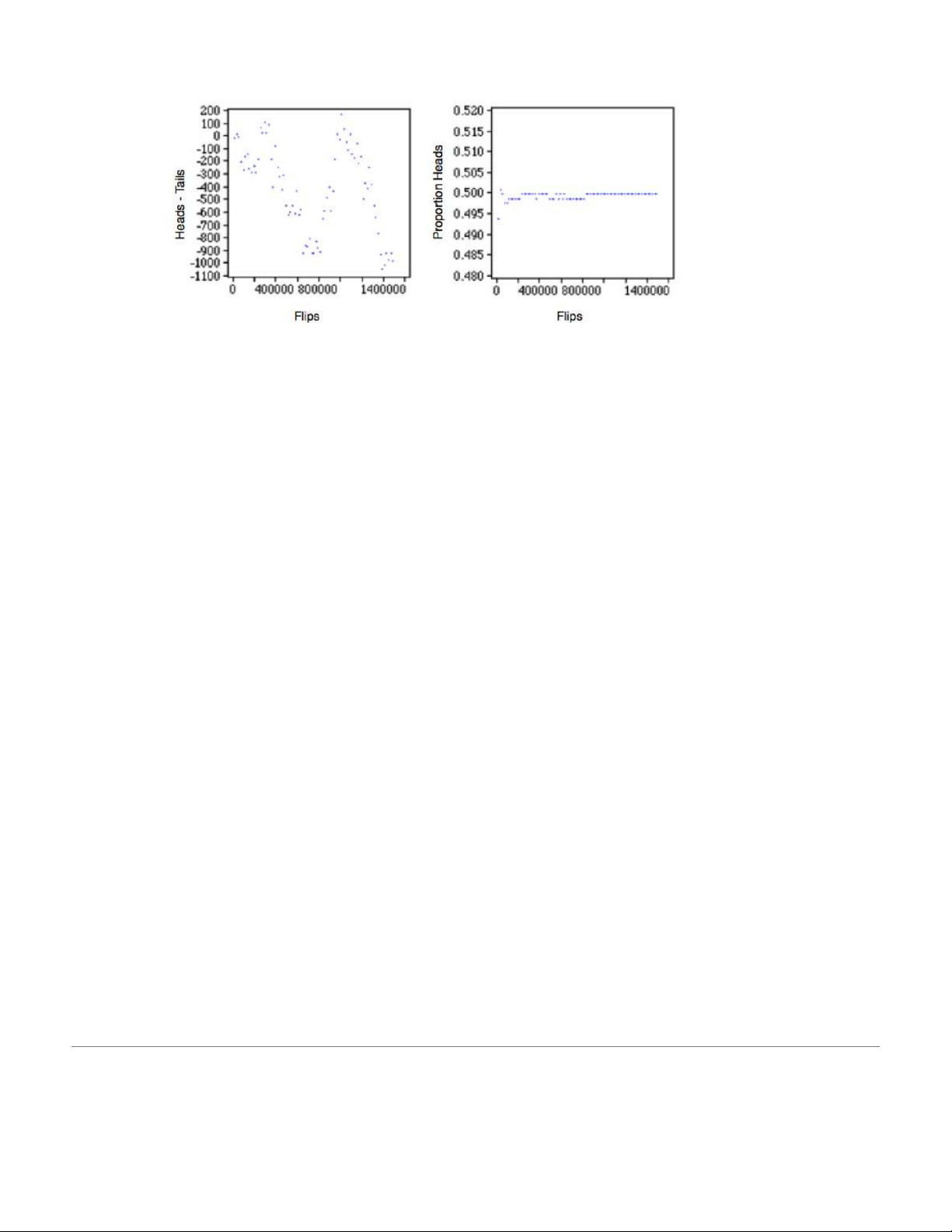
Figure 1. The results of simulating 1,500,000 coin flips. The graph on the left
shows the difference between the number of heads and the number of tails as
a function of the number of flips. You can see that there is no consistent
pattern. After the final flip, there are 968 more tails than heads. The graph on
the right shows the proportion of heads. This value goes up and down at the
beginning, but converges to 0.5 (rounded to 3 decimal places) before 1,000,000 flips. 197
Permutations and Combinations by David M. Lane Prerequisites none Learning Objectives
1. Calculate the probability of two independent events occurring
2. Define permutations and combinations
3. List all permutations and combinations
4. Apply formulas for permutations and combinations
This section covers basic formulas for determining the number of various possible
types of outcomes. The topics covered are: (1) counting the number of possible
orders, (2) counting using the multiplication rule, (3) counting the number of
permutations, and (4) counting the number of combinations. Possible Orders
Suppose you had a plate with three pieces of candy on it: one green, one yellow,
and one red. You are going to pick up these three pieces one at a time. The question
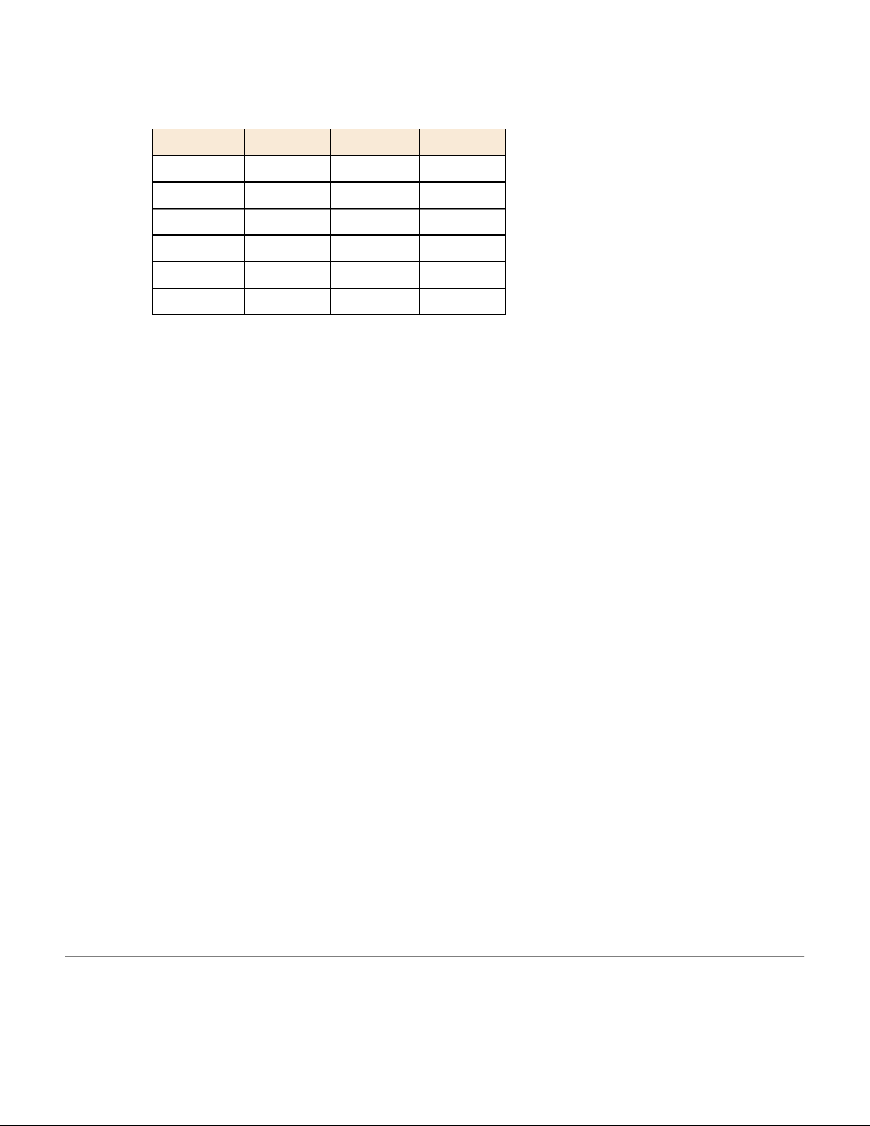
is: In how many different orders can you pick up the pieces? Table 1 lists all the
possible orders. There are two orders in which red is first: red, yellow, green and
red, green, yellow. Similarly, there are two orders in which yellow is first and two
orders in which green is first. This makes six possible orders in which the pieces can be picked up. 198 Table 1. Six Possible Orders. Number First Second Third 1 red yellow green 2 red green yellow 3 yellow red green 4 yellow green red 5 green red yellow 6 green yellow red
The formula for the number of orders is shown below. Number of orders = n!
where n is the number of pieces to be picked up. The symbol “!” stands for factorial. Some examples are: 3! = 3 x 2 x 1 = 6 4! = 4 x 3 x 2 x 1 = 24 5! = 5 x 4 x 3 x 2 x 1 = 120
This means that if there were 5 pieces of candy to be picked up, they could be
picked up in any of 5! = 120 orders. Multiplication Rule
Imagine a small restaurant whose menu has 3 soups, 6 entrées, and 4 desserts. How
many possible meals are there? The answer is calculated by multiplying the
numbers to get 3 x 6 x 4 = 72. You can think of it as first there is a choice among 3
soups. Then, for each of these choices there is a choice among 6 entrées resulting
in 3 x 6 = 18 possibilities. Then, for each of these 18 possibilities there are 4
possible desserts yielding 18 x 4 = 72 total possibilities. Permutations
Suppose that there were four pieces of candy (red, yellow, green, and brown) and
you were only going to pick up exactly two pieces. How many ways are there of 199
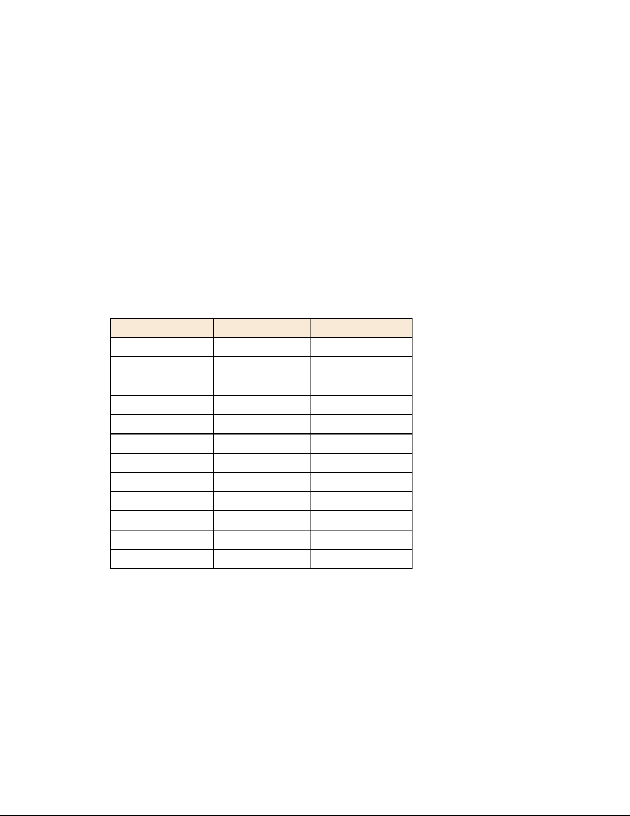
picking up two pieces? Table 2 lists all the possibilities. The first choice can be any
of the four colors. For each of these 4 first choices there are 3 second choices.
Therefore there are 4 x 3 = 12 possibilities.
Table 2. Twelve Possible Orders. Number First Second 1 red yellow 2 red green 3 red brown 4 yellow red 5 yellow green 6 yellow brown 7 green red 8 green yellow 9 green brown 10 brown red 11 brown yellow 12 brown green
More formally, this question is asking for the number of permutations of four
things taken two at a time. The general formula is: P(n r) !n! n r =-
where nPr is the number of permutations of n things taken r at a time. In other
words, it is the number of ways r things can be selected from a group of n things. In this case, 4 2 =- 4 = = P( ) ! ! 4 x 3 x 2 x 1 12 4 2 2 x 1
It is important to note that order counts in permutations. That is, choosing red and
then yellow is counted separately from choosing yellow and then red. Therefore
permutations refer to the number of ways of choosing rather than the number of 200
possible outcomes. When order of choice is not considered, the formula for combinations is used. Combinations
Now suppose that you were not concerned with the way the pieces of candy were
chosen but only in the final choices. In other words, how many different
combinations of two pieces could you end up with? In counting combinations,
choosing red and then yellow is the same as choosing yellow and then red because
in both cases you end up with one red piece and one yellow piece. Unlike
permutations, order does not count. Table 3 is based on Table 2 but is modified so
that repeated combinations are given an “x” instead of a number. For example,
“yellow then red” has an “x” because the combination of red and yellow was
already included as choice number 1. As you can see, there are six combinations of the three colors. Table 3. Six Combinations. Number First Second 1 red yellow 2 red green 3 red brown x yellow red 4 yellow green 5 yellow brown x green red x green yellow 6 green brown x brown red x brown yellow x brown green
The formula for the number of combinations is shown below where nCr is the
number of combinations for n things taken r at a time. 201 n! C n r (n r) ! r =- ! For our example, 4 C4 2 2 ! ! (4 x 3) ( x 2 x )1 4 2 =-= = 6 ( ) ! 2 x 1 2 1 x
which is consistent with Table 3.
As an example application, suppose there were six kinds of toppings that one could
order for a pizza. How many combinations of exactly 3 toppings could be ordered?
Here n = 6 since there are 6 toppings and r = 3 since we are taking 3 at a time. The formula is then: 6! 6 x 5 x 4 x 3 x 2 x 1 6 3 =-= = !20. ( ) ! (3 x 2 x 1)(3 x 2 x 1) 202 Binomial Distribution by David M. Lane Prerequisites
•Chapter 1: Distributions •Chapter 3: Variability
•Chapter 5: Basic Probability Learning Objectives
1. Define binomial outcomes
2. Compute the probability of getting X successes in N trials
3. Compute cumulative binomial probabilities
4. Find the mean and standard deviation of a binomial distribution
When you flip a coin, there are two possible outcomes: heads and tails. Each
outcome has a fixed probability, the same from trial to trial. In the case of coins,
heads and tails each have the same probability of 1/2. More generally, there are
situations in which the coin is biased, so that heads and tails have different
probabilities. In the present section, we consider probability distributions for which
there are just two possible outcomes with fixed probabilities summing to one.
These distributions are called binomial distributions. A Simple Example
The four possible outcomes that could occur if you flipped a coin twice are listed
below in Table 1. Note that the four outcomes are equally likely: each has
probability 1/4. To see this, note that the tosses of the coin are independent (neither
affects the other). Hence, the probability of a head on Flip 1 and a head on Flip 2 is
the product of P(H) and P(H), which is 1/2 x 1/2 = 1/4. The same calculation
applies to the probability of a head on Flip 1 and a tail on Flip 2. Each is 1/2 x 1/2 = 1/4.
Table 1. Four Possible Outcomes. Outcome First Flip Second Flip 1 Heads Heads 2 Heads Tails 203 3 Tails Heads 4 Tails Tails
The four possible outcomes can be classified in terms of the number of heads that
come up. The number could be two (Outcome 1), one (Outcomes 2 and 3) or 0
(Outcome 4). The probabilities of these possibilities are shown in Table 2 and in
Figure 1. Since two of the outcomes represent the case in which just one head
appears in the two tosses, the probability of this event is equal to 1/4 + 1/4 = 1/2.
Table 2 summarizes the situation.
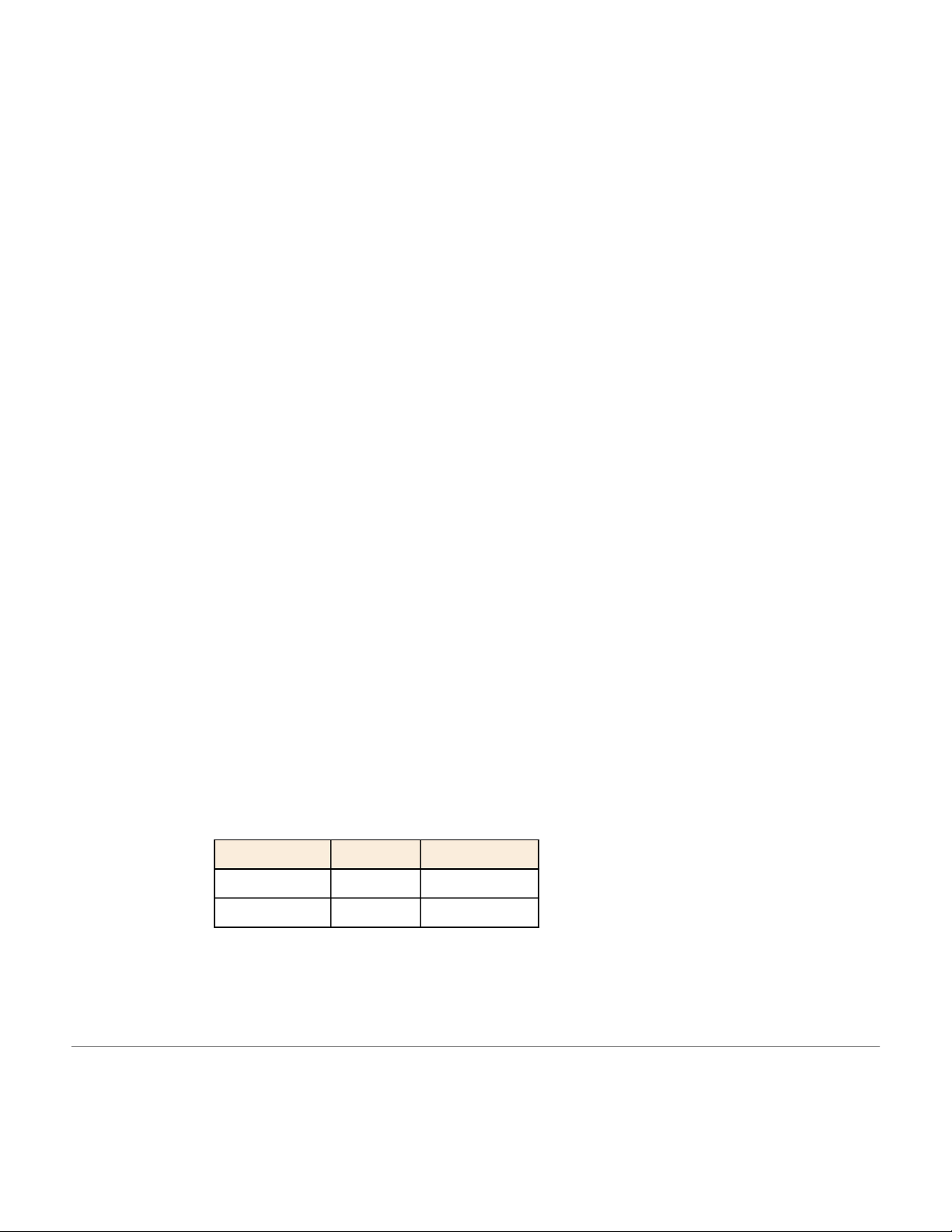
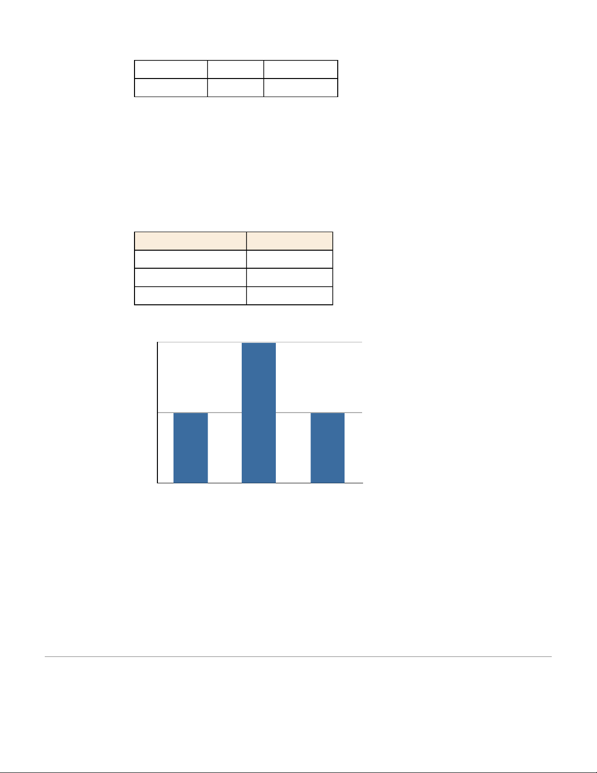
Table 2. Probabilities of Getting 0, 1, or 2 Heads. Number of Heads Probability 0 1/4 1 1/2 2 1/4 0.5 0.25 Probability 0 012 Number3of3Heads
Figure 1. Probabilities of 0, 1, and 2 heads.
Figure 1 is a discrete probability distribution: It shows the probability for each of
the values on the X-axis. Defining a head as a “success,” Figure 1 shows the
probability of 0, 1, and 2 successes for two trials (flips) for an event that has a 204