ELT3047 Computer Architecture
Lesson 2: Performance measurement Hoang Gia Hung
Faculty of Electronics and Telecommunications
University of Engineering and Technology, VNU Hanoi Last lesson review
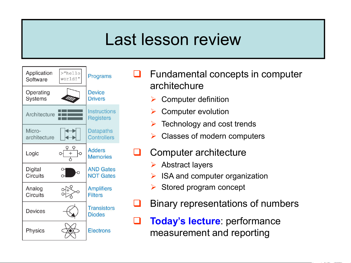
❑ Fundamental concepts in computer architechure ➢ Computer definition ➢ Computer evolution ➢ Technology and cost trends
➢ Classes of modern computers ❑ Computer architecture ➢ Abstract layers
➢ ISA and computer organization ➢ Stored program concept
❑ Binary representations of numbers
❑ Today’s lecture: performance measurement and reporting
Why do we need measuring computer performance?
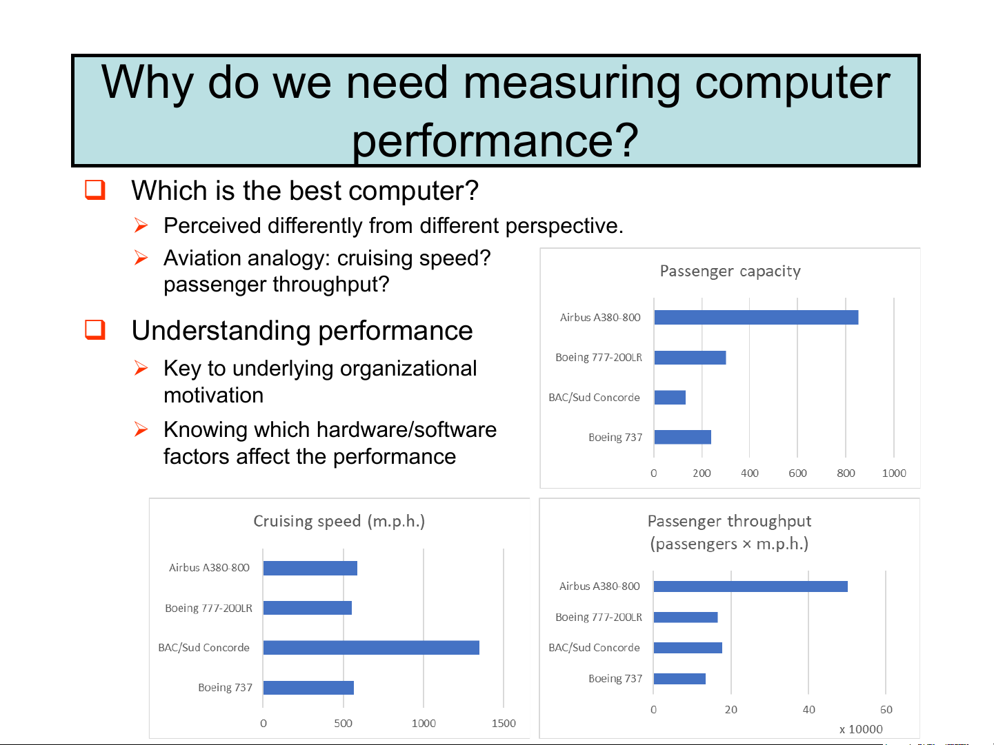
❑ Which is the best computer?
➢ Perceived differently from different perspective.
➢ Aviation analogy: cruising speed? passenger throughput? ❑ Understanding performance
➢ Key to underlying organizational motivation
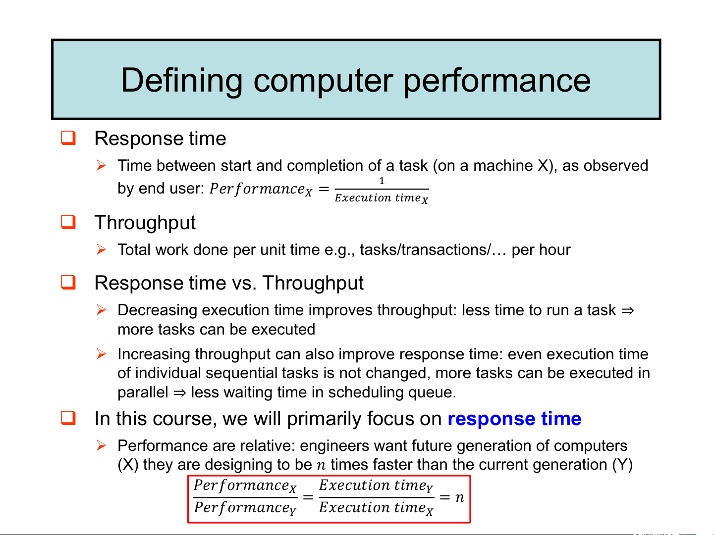
➢ Knowing which hardware/software factors affect the performance Defining computer performance ❑ Response time
➢ Time between start and completion of a task (on a machine X), as observed
by end user: 𝑃𝑒𝑟𝑓𝑜𝑟𝑚𝑎𝑛𝑐𝑒𝑋 = 1
𝐸𝑥𝑒𝑐𝑢𝑡𝑖𝑜𝑛 𝑡𝑖𝑚𝑒𝑋 ❑ Throughput
➢ Total work done per unit time e.g., tasks/transactions/… per hour
❑ Response time vs. Throughput
➢ Decreasing execution time improves throughput: less time to run a task ⇒ more tasks can be executed
➢ Increasing throughput can also improve response time: even execution time
of individual sequential tasks is not changed, more tasks can be executed in
parallel ⇒ less waiting time in scheduling queue.
❑ In this course, we will primarily focus on response time
➢ Performance are relative: engineers want future generation of computers
(X) they are designing to be 𝑛 times faster than the current generation (Y)
𝑃𝑒𝑟𝑓𝑜𝑟𝑚𝑎𝑛𝑐𝑒𝑋 𝐸𝑥𝑒𝑐𝑢𝑡𝑖𝑜𝑛 𝑡𝑖𝑚𝑒𝑌
𝑃𝑒𝑟𝑓𝑜𝑟𝑚𝑎𝑛𝑐𝑒 = = 𝑛 𝑌
𝐸𝑥𝑒𝑐𝑢𝑡𝑖𝑜𝑛 𝑡𝑖𝑚𝑒𝑋 Measuring Execution Time
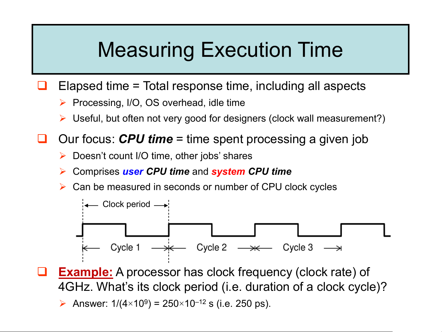
❑ Elapsed time = Total response time, including all aspects
➢ Processing, I/O, OS overhead, idle time
➢ Useful, but often not very good for designers (clock wall measurement?)
❑ Our focus: CPU time = time spent processing a given job
➢ Doesn’t count I/O time, other jobs’ shares
➢ Comprises user CPU time and system CPU time
➢ Can be measured in seconds or number of CPU clock cycles Clock period
❑ Example: A processor has clock frequency (clock rate) of
4GHz. What’s its clock period (i.e. duration of a clock cycle)?
➢ Answer: 1/(4×109) = 250×10–12 s (i.e. 250 ps).
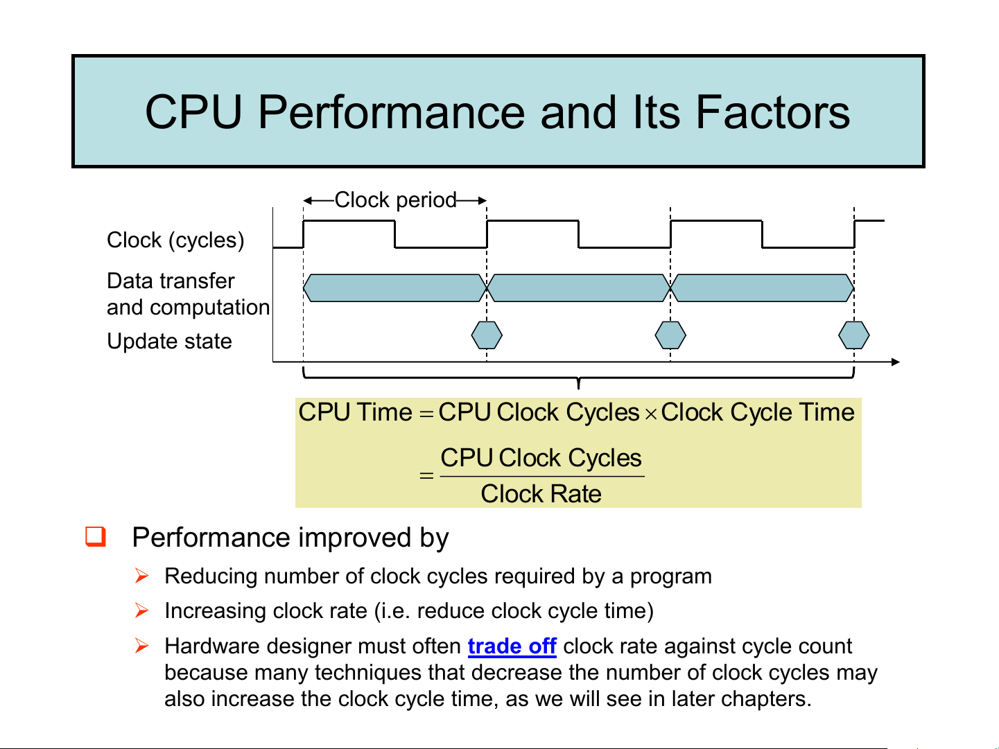
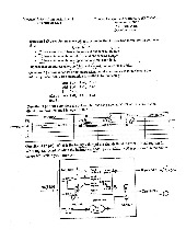
CPU Performance and Its Factors Clock period Clock (cycles) Data transfer and computation Update state CPU T ime = CPU C lock C ycles  Clock C ycle T ime CPU C lock C ycles = Clock R ate ❑ Performance improved by
➢ Reducing number of clock cycles required by a program
➢ Increasing clock rate (i.e. reduce clock cycle time)
➢ Hardware designer must often trade off clock rate against cycle count
because many techniques that decrease the number of clock cycles may
also increase the clock cycle time, as we will see in later chapters. CPU Time Example
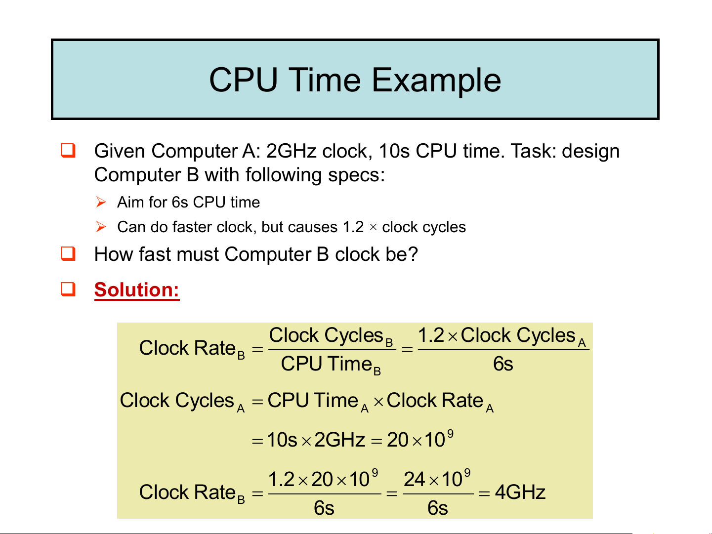
❑ Given Computer A: 2GHz clock, 10s CPU time. Task: design
Computer B with following specs: ➢ Aim for 6s CPU time
➢ Can do faster clock, but causes 1.2 × clock cycles
❑ How fast must Computer B clock be? ❑ Solution: Clock Cy cles 1.2  Clock Cy cles Clock Ra te B A = = B CPU Tim e 6s B Clock Cy cles = CPU Tim e  Clock Ra te A A A = 10s 2GHz = 20 109 1.2  20 109 24 109 Clock Ra te = = = 4GHz B 6s 6s Instruction Count and CPI
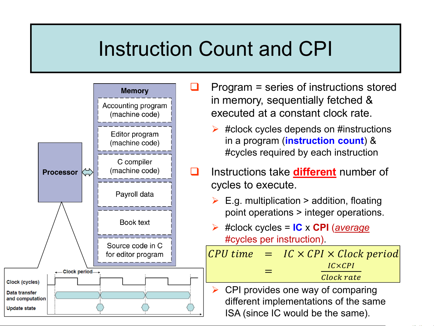
❑ Program = series of instructions stored
in memory, sequentially fetched &
executed at a constant clock rate.
➢ #clock cycles depends on #instructions
in a program (instruction count) &
#cycles required by each instruction
❑ Instructions take different number of cycles to execute.
➢ E.g. multiplication > addition, floating
point operations > integer operations.
➢ #clock cycles = IC x CPI (average #cycles per instruction).
𝐶𝑃𝑈 𝑡𝑖𝑚𝑒 = 𝐼𝐶 × 𝐶𝑃𝐼 × 𝐶𝑙𝑜𝑐𝑘 𝑝𝑒𝑟𝑖𝑜𝑑 = 𝐼𝐶×𝐶𝑃𝐼
𝐶𝑙𝑜𝑐𝑘 𝑟𝑎𝑡𝑒
➢ CPI provides one way of comparing
different implementations of the same
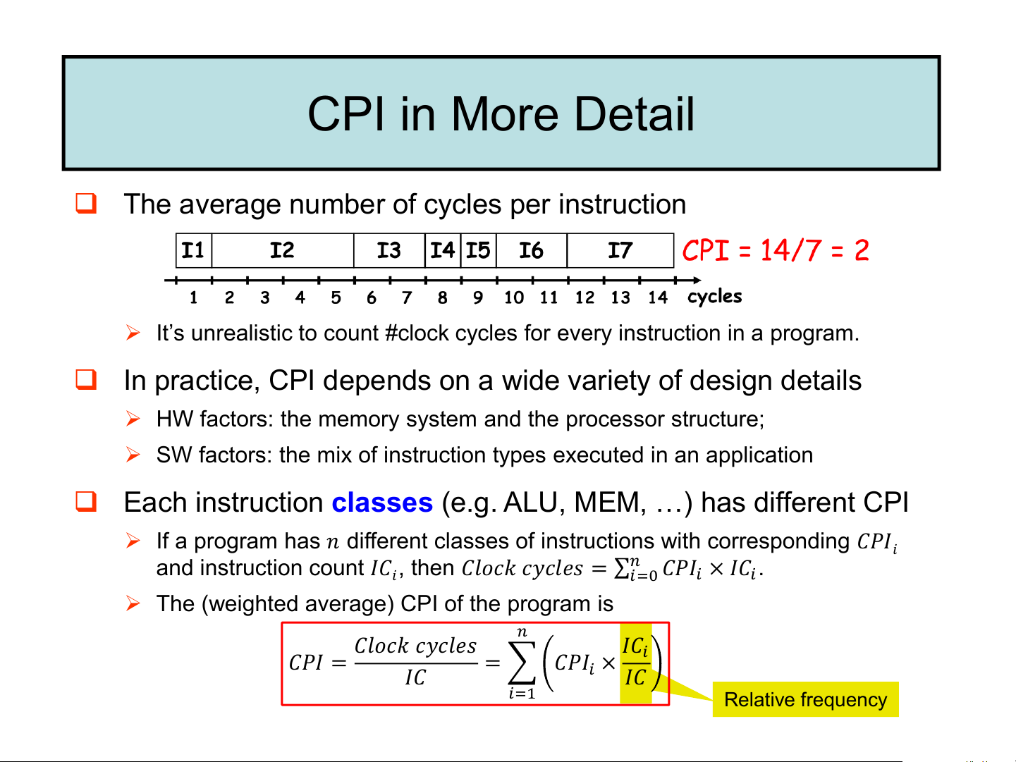
ISA (since IC would be the same). CPI in More Detail
❑ The average number of cycles per instruction
➢ It’s unrealistic to count #clock cycles for every instruction in a program.
❑ In practice, CPI depends on a wide variety of design details
➢ HW factors: the memory system and the processor structure;
➢ SW factors: the mix of instruction types executed in an application
❑ Each instruction classes (e.g. ALU, MEM, …) has different CPI
➢ If a program has 𝑛 different classes of instructions with corresponding 𝐶𝑃𝐼𝑖 and instruction count 𝐼𝐶 𝑛
𝑖, then 𝐶𝑙𝑜𝑐𝑘 𝑐𝑦𝑐𝑙𝑒𝑠 = σ𝑖=0 𝐶𝑃𝐼𝑖 × 𝐼𝐶𝑖.
➢ The (weighted average) CPI of the program is
𝐶𝑙𝑜𝑐𝑘 𝑐𝑦𝑐𝑙𝑒𝑠 𝑛 𝐼𝐶 𝐶𝑃𝐼 = 𝑖 𝐼𝐶
= ෍ 𝐶𝑃𝐼𝑖 × 𝐼𝐶 𝑖=1 Relative frequency CPI Example
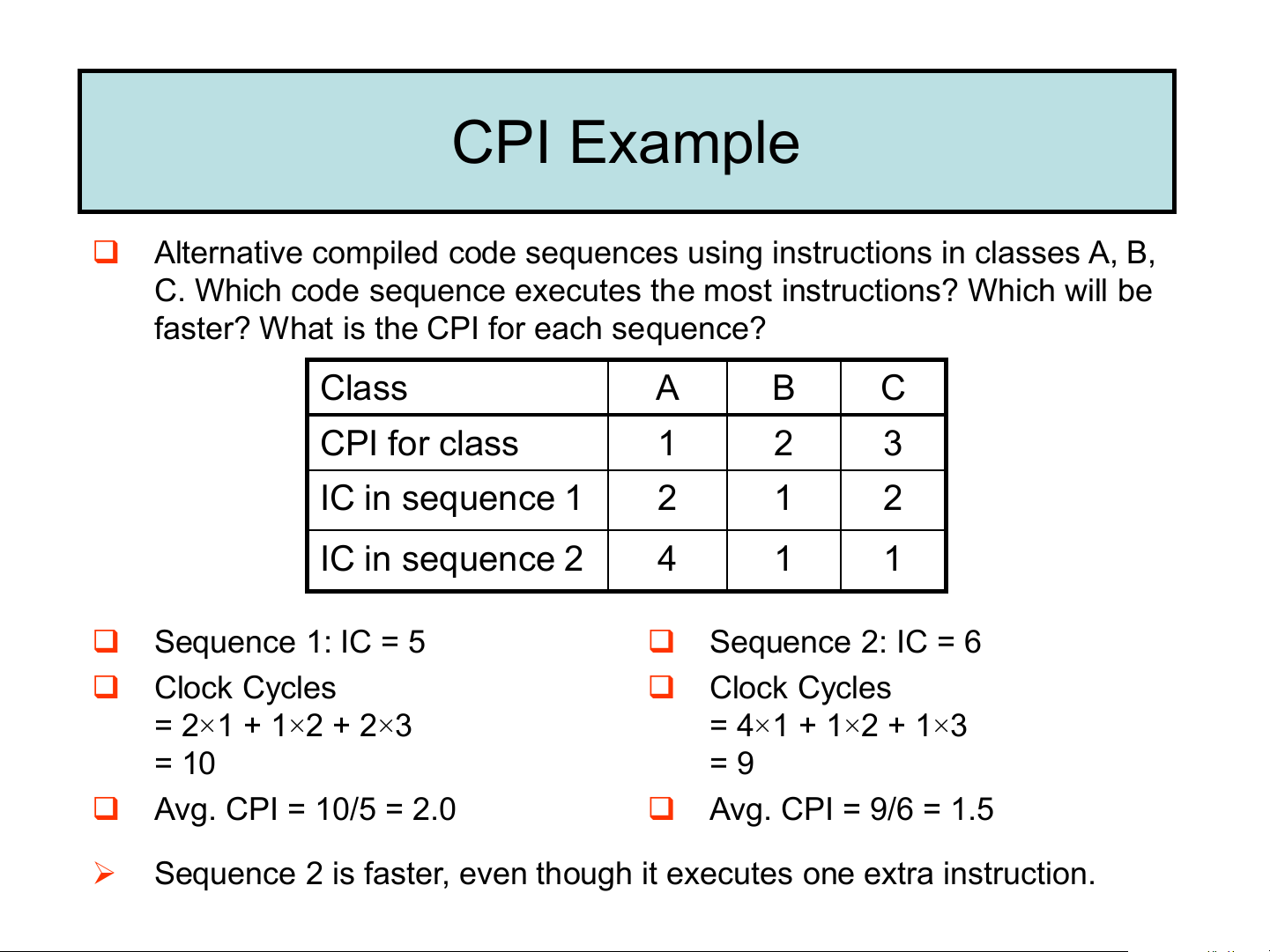
❑ Alternative compiled code sequences using instructions in classes A, B,
C. Which code sequence executes the most instructions? Which will be
faster? What is the CPI for each sequence? Class A B C CPI for class 1 2 3 IC in sequence 1 2 1 2 IC in sequence 2 4 1 1 ❑ Sequence 1: IC = 5 ❑ Sequence 2: IC = 6 ❑ Clock Cycles ❑ Clock Cycles = 2×1 + 1×2 + 2×3 = 4×1 + 1×2 + 1×3 = 10 = 9 ❑ Avg. CPI = 10/5 = 2.0 ❑ Avg. CPI = 9/6 = 1.5 ➢
Sequence 2 is faster, even though it executes one extra instruction. Performance summary
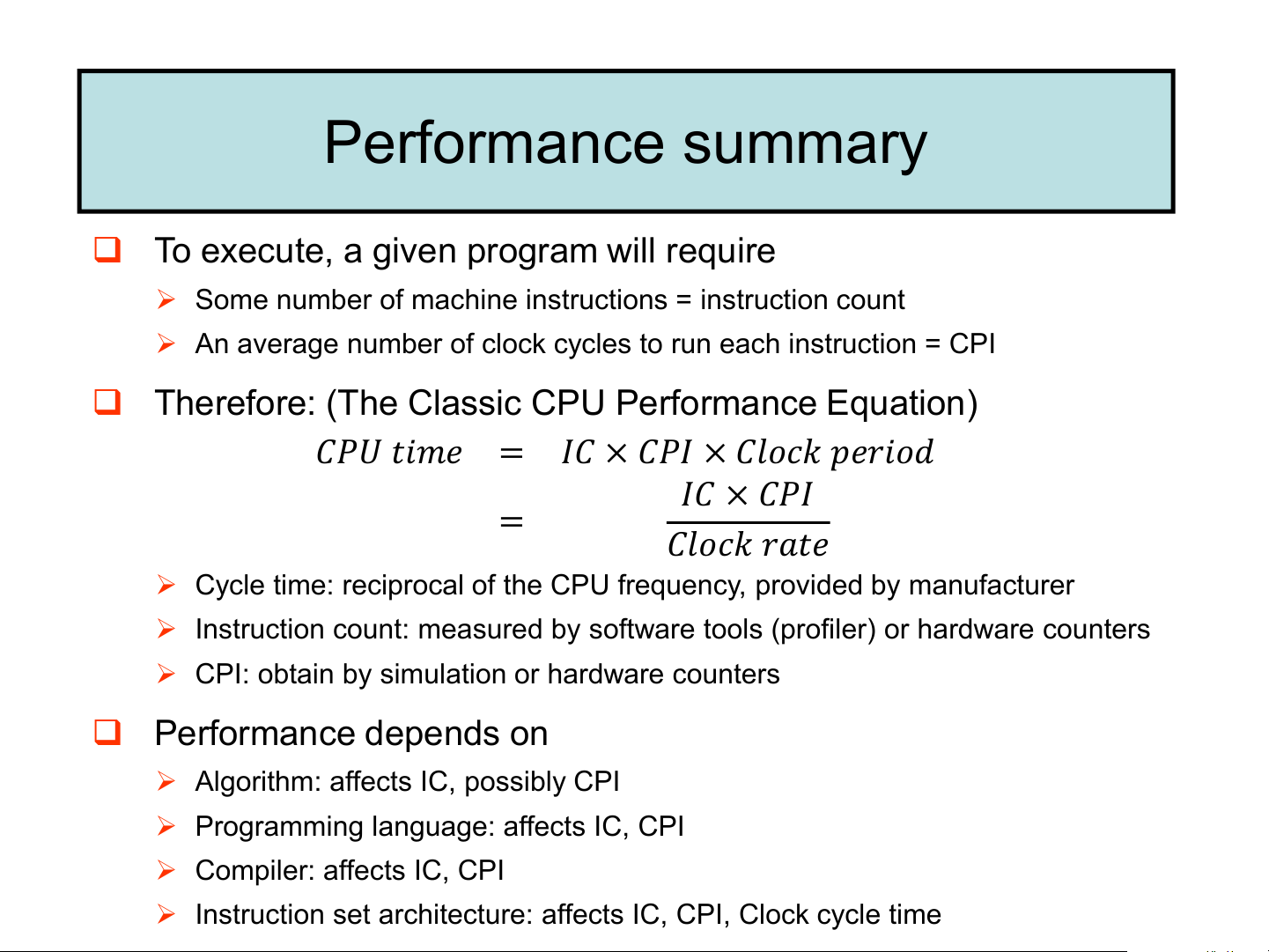
❑ To execute, a given program will require
➢ Some number of machine instructions = instruction count
➢ An average number of clock cycles to run each instruction = CPI
❑ Therefore: (The Classic CPU Performance Equation)
𝐶𝑃𝑈 𝑡𝑖𝑚𝑒 = 𝐼𝐶 × 𝐶𝑃𝐼 × 𝐶𝑙𝑜𝑐𝑘 𝑝𝑒𝑟𝑖𝑜𝑑 𝐼𝐶 × 𝐶𝑃𝐼 =
𝐶𝑙𝑜𝑐𝑘 𝑟𝑎𝑡𝑒
➢ Cycle time: reciprocal of the CPU frequency, provided by manufacturer
➢ Instruction count: measured by software tools (profiler) or hardware counters
➢ CPI: obtain by simulation or hardware counters ❑ Performance depends on
➢ Algorithm: affects IC, possibly CPI
➢ Programming language: affects IC, CPI ➢ Compiler: affects IC, CPI
➢ Instruction set architecture: affects IC, CPI, Clock cycle time Performance Example 1
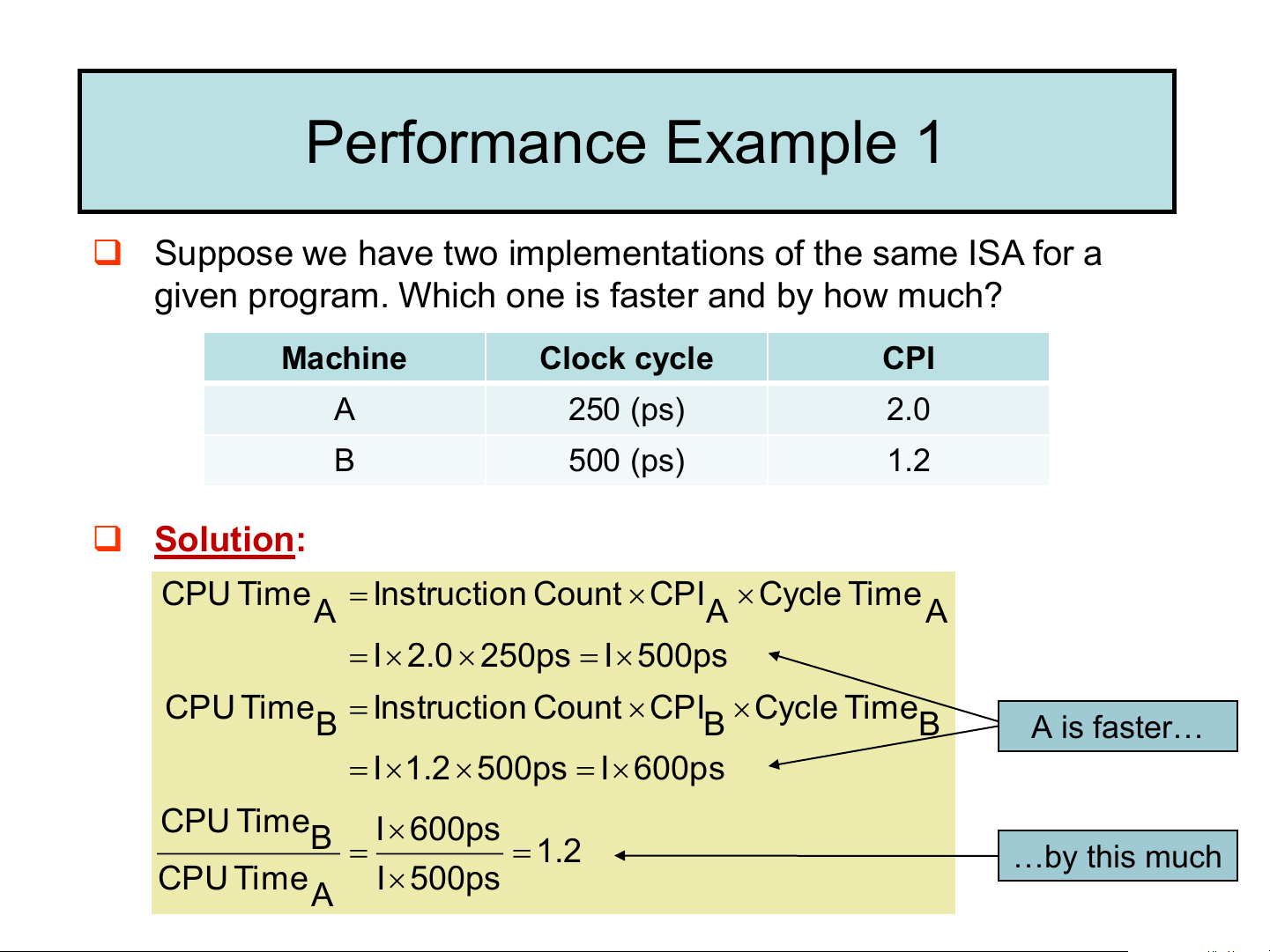
❑ Suppose we have two implementations of the same ISA for a
given program. Which one is faster and by how much? Machine Clock cycle CPI A 250 (ps) 2.0 B 500 (ps) 1.2 ❑ Solution: CPU T ime = Instructio C n ount  CPI  Cycle T ime A A A
= I 2.0 250ps = I500ps CPU T ime = Instructio C n ount  CPI  Cycle T ime B B B A is faster… = I1.2500ps = I 600ps CPU T ime I 600ps B = = 1.2 …by this much CPU T ime I 500ps A Performance Example 2
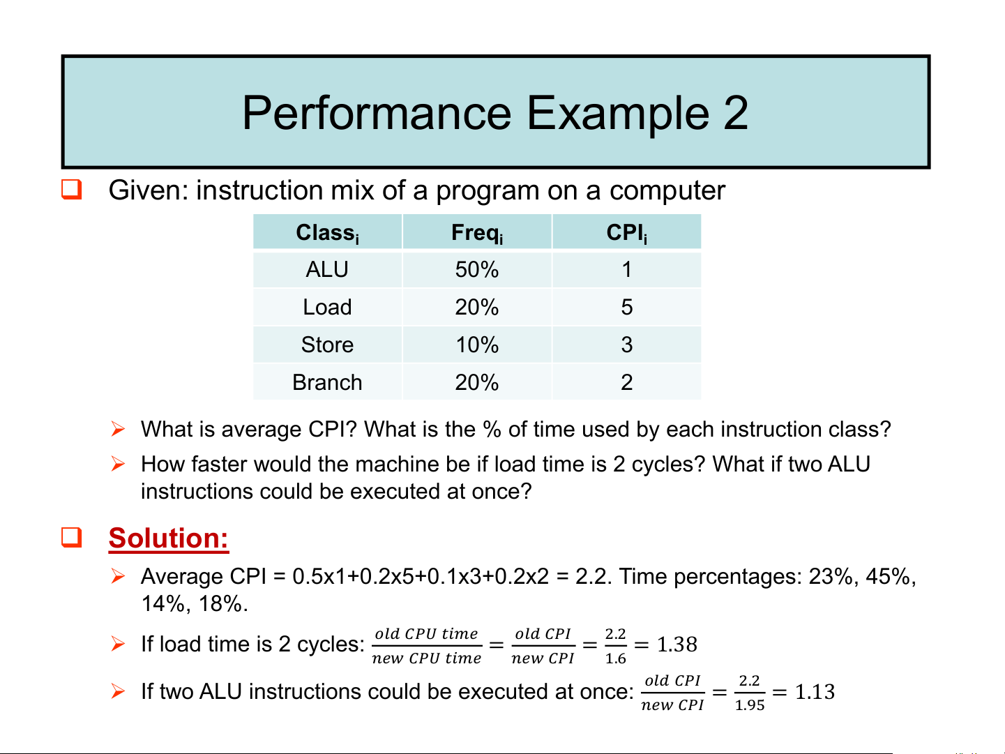
❑ Given: instruction mix of a program on a computer Class Freq CPI i i i ALU 50% 1 Load 20% 5 Store 10% 3 Branch 20% 2
➢ What is average CPI? What is the % of time used by each instruction class?
➢ How faster would the machine be if load time is 2 cycles? What if two ALU
instructions could be executed at once? ❑ Solution:
➢ Average CPI = 0.5x1+0.2x5+0.1x3+0.2x2 = 2.2. Time percentages: 23%, 45%, 14%, 18%. ➢
𝑜𝑙𝑑 𝐶𝑃𝑈 𝑡𝑖𝑚𝑒 If load time is 2 cycles:
= 𝑜𝑙𝑑 𝐶𝑃𝐼 = 2.2 = 1.38
𝑛𝑒𝑤 𝐶𝑃𝑈 𝑡𝑖𝑚𝑒 𝑛𝑒𝑤 𝐶𝑃𝐼 1.6 ➢ 𝑜𝑙𝑑 𝐶𝑃𝐼
If two ALU instructions could be executed at once: = 2.2 = 1.13 𝑛𝑒𝑤 𝐶𝑃𝐼 1.95
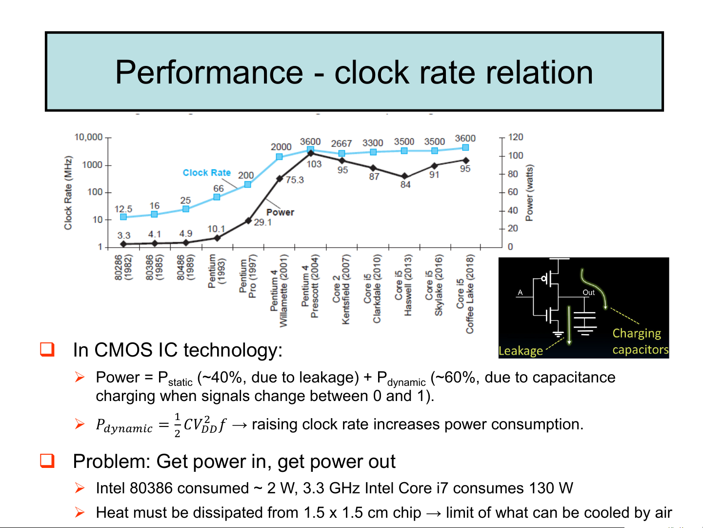
Performance - clock rate relation ❑ In CMOS IC technology: ➢ Power = P (~40%, due to leakage) + P (~60%, due to capacitance static dynamic
charging when signals change between 0 and 1). ➢ 𝑃 2
𝑑𝑦𝑛𝑎𝑚𝑖𝑐 = 1 𝐶𝑉 𝑓 → raising clock rate increases power consumption. 2 𝐷𝐷
❑ Problem: Get power in, get power out
➢ Intel 80386 consumed ~ 2 W, 3.3 GHz Intel Core i7 consumes 130 W
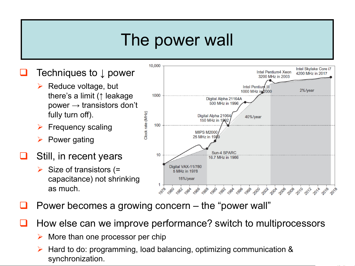
➢ Heat must be dissipated from 1.5 x 1.5 cm chip → limit of what can be cooled by air The power wall ❑ Techniques to ↓ power ➢ Reduce voltage, but
there’s a limit (↑ leakage power → transistors don’t fully turn off). ➢ Frequency scaling ➢ Power gating ❑ Still, in recent years ➢ Size of transistors (= capacitance) not shrinking as much.
❑ Power becomes a growing concern – the “power wall”
❑ How else can we improve performance? switch to multiprocessors
➢ More than one processor per chip
➢ Hard to do: programming, load balancing, optimizing communication & synchronization. MIPS as a Performance Metric
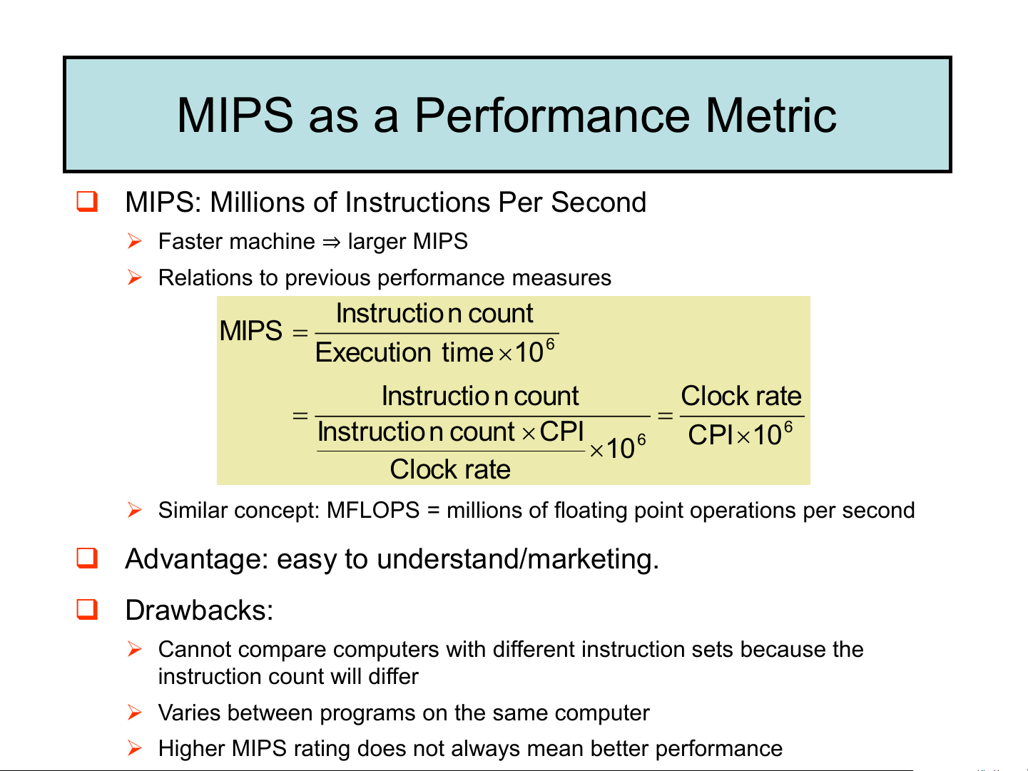
❑ MIPS: Millions of Instructions Per Second
➢ Faster machine ⇒ larger MIPS
➢ Relations to previous performance measures Instructio c n ount MIPS = 6 Execution t ime 10 Instructio c n ount Clock r ate = = 6 Instructio c n ount  CPI 6 CPI10 10 Clock r ate
➢ Similar concept: MFLOPS = millions of floating point operations per second
❑ Advantage: easy to understand/marketing. ❑ Drawbacks:
➢ Cannot compare computers with different instruction sets because the instruction count will differ
➢ Varies between programs on the same computer
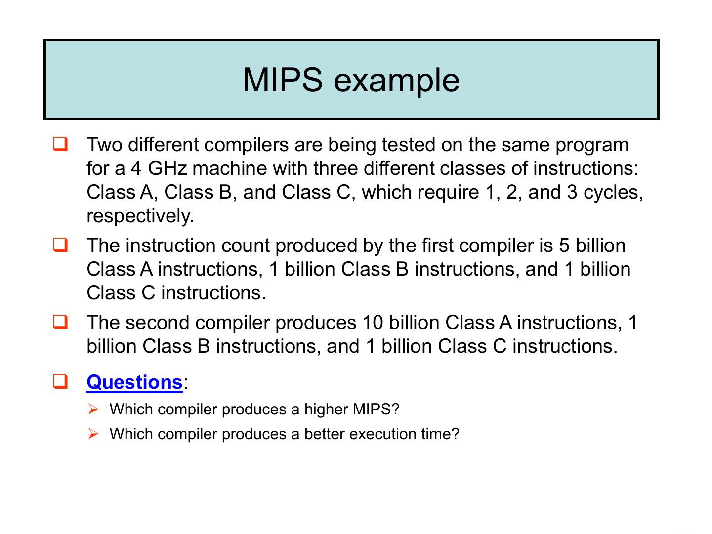
➢ Higher MIPS rating does not always mean better performance MIPS example
❑ Two different compilers are being tested on the same program
for a 4 GHz machine with three different classes of instructions:
Class A, Class B, and Class C, which require 1, 2, and 3 cycles, respectively.
❑ The instruction count produced by the first compiler is 5 billion
Class A instructions, 1 billion Class B instructions, and 1 billion Class C instructions.
❑ The second compiler produces 10 billion Class A instructions, 1
billion Class B instructions, and 1 billion Class C instructions. ❑ Questions:
➢ Which compiler produces a higher MIPS?
➢ Which compiler produces a better execution time? MIPS example solution
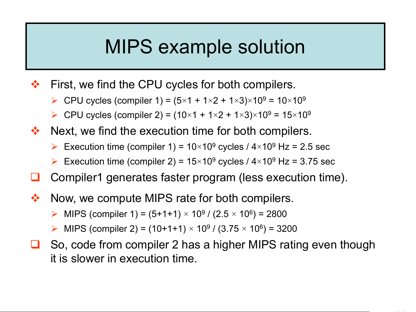
❖ First, we find the CPU cycles for both compilers.
➢ CPU cycles (compiler 1) = (5×1 + 1×2 + 1×3)×109 = 10×109
➢ CPU cycles (compiler 2) = (10×1 + 1×2 + 1×3)×109 = 15×109
❖ Next, we find the execution time for both compilers.
➢ Execution time (compiler 1) = 10×109 cycles / 4×109 Hz = 2.5 sec
➢ Execution time (compiler 2) = 15×109 cycles / 4×109 Hz = 3.75 sec
❑ Compiler1 generates faster program (less execution time).
❖ Now, we compute MIPS rate for both compilers.
➢ MIPS (compiler 1) = (5+1+1) × 109 / (2.5 × 106) = 2800
➢ MIPS (compiler 2) = (10+1+1) × 109 / (3.75 × 106) = 3200
❑ So, code from compiler 2 has a higher MIPS rating even though
it is slower in execution time. Amdahl’s Law
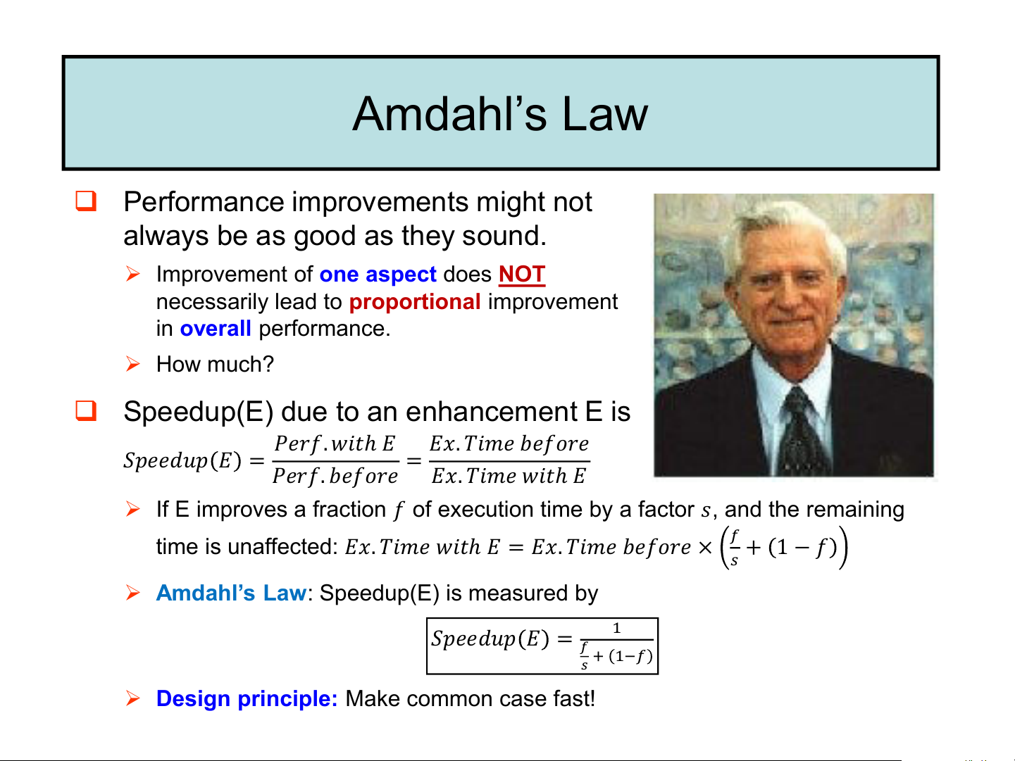
❑ Performance improvements might not
always be as good as they sound.
➢ Improvement of one aspect does NOT
necessarily lead to proportional improvement in overall performance. ➢ How much?
❑ Speedup(E) due to an enhancement E is
𝑃𝑒𝑟𝑓. 𝑤𝑖𝑡ℎ 𝐸
𝐸𝑥. 𝑇𝑖𝑚𝑒 𝑏𝑒𝑓𝑜𝑟𝑒
𝑆𝑝𝑒𝑒𝑑𝑢𝑝 𝐸 = 𝑃𝑒𝑟𝑓.𝑏𝑒𝑓𝑜𝑟𝑒 = 𝐸𝑥.𝑇𝑖𝑚𝑒 𝑤𝑖𝑡ℎ 𝐸
➢ If E improves a fraction 𝑓 of execution time by a factor 𝑠, and the remaining
time is unaffected: 𝐸𝑥. 𝑇𝑖𝑚𝑒 𝑤𝑖𝑡ℎ 𝐸 = 𝐸𝑥. 𝑇𝑖𝑚𝑒 𝑏𝑒𝑓𝑜𝑟𝑒 × 𝑓 + 1 − 𝑓 𝑠
➢ Amdahl’s Law: Speedup(E) is measured by
𝑆𝑝𝑒𝑒𝑑𝑢𝑝 𝐸 = 1 𝑓𝑠 + 1−𝑓
➢ Design principle: Make common case fast! Amdahl’s Law example
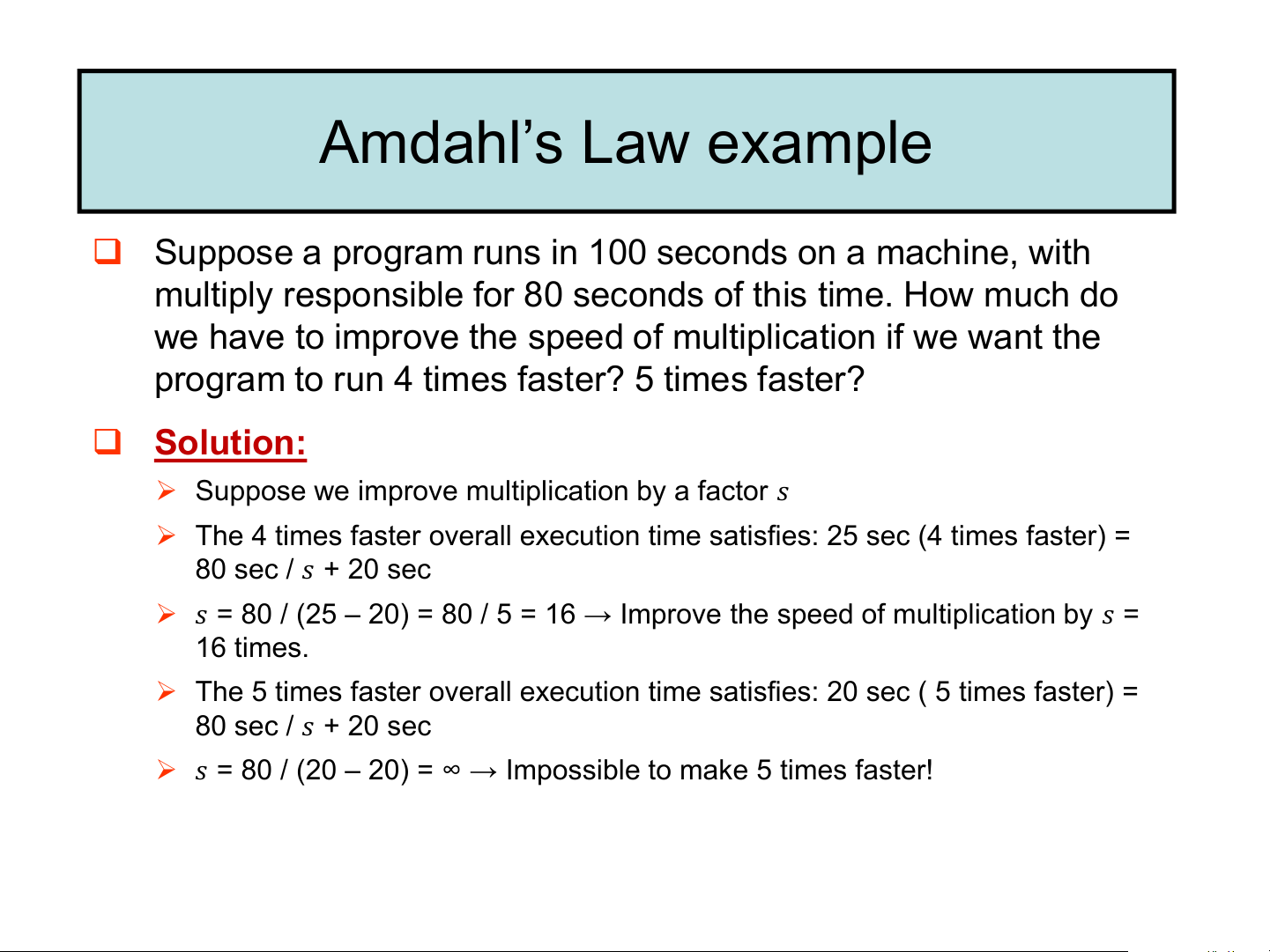
❑ Suppose a program runs in 100 seconds on a machine, with
multiply responsible for 80 seconds of this time. How much do
we have to improve the speed of multiplication if we want the
program to run 4 times faster? 5 times faster? ❑ Solution:
➢ Suppose we improve multiplication by a factor 𝑠
➢ The 4 times faster overall execution time satisfies: 25 sec (4 times faster) = 80 sec / 𝑠 + 20 sec
➢ 𝑠 = 80 / (25 – 20) = 80 / 5 = 16 → Improve the speed of multiplication by 𝑠 = 16 times.
➢ The 5 times faster overall execution time satisfies: 20 sec ( 5 times faster) = 80 sec / 𝑠 + 20 sec
➢ 𝑠 = 80 / (20 – 20) = ∞ → Impossible to make 5 times faster!