Statistical exercises: mean & variance of continuous random variables môn Xác suất thống kê| Trường Đại học Ngoại Thương
Firstly, we should confirm the validity and domain of the f(x). - Secondly, we find the mean, i.e., the expected value of X. - Finally, we find the variance of X. Tài liệu giúp bạn tham khảo, ôn tập và đạt kết quả cao. Mời đọc đón xem!
Môn: Xác suất thống kê (FTU) 355 tài liệu
Trường: Trường Đại học Ngoại Thương 1.1 K tài liệu
Tác giả:


Preview text:
08:46, 28/01/2026
Statistical Exercises: Mean & Variance of Continuous Random Variables - Studocu
Exercise 2.5 Find the mean and variance of X with density 𝑓(𝑥) 1
𝜆 exp (− 𝑥𝜆) suggests an exponental distribution so X is a continuous random The given 𝑓(𝑥)=1 va X r iia s:b
le and f(x) is a probability density function. The approach to find the mean and variance of
- Firstly, we should confirm the validity and domain of the f(x).
- Secondly, we find the mean, i.e., the expected value of X.
- Finally, we find the variance of X. + Co 𝜆n fi m r u m st t b h e eg v r a e ltid er i tty h aan n d z e d r o o m bea c in au o s f e: t he f(x)
- If 𝜆 < 0 => 𝑓(𝑥)< 0. Invalid because f(x) must be non-negative.
- If 𝜆 = 0 => 1 𝜆 is undefined. 𝜆exp (− 𝑥
Because f(x) is an exponential distribution so its support must be 𝑥 ≥ 0. A 𝜆 p ) ro 𝑑 b 𝑥 ability density
function (PDF) must integrate to 1 over its support. Let’s check ∫1
𝜆, so 𝑥 = 𝜆𝑡, 𝑑𝑥 = 𝜆𝑑 0 𝑡.
∞ Adjust the limits: whe0n. 𝑥 = −0, 𝑡 = 0; when 𝑥 → ∞ Substitute 𝑡 = 𝑥
∫10∫exp(−𝑡)𝑑𝑡 =[−exp (−𝑡)]
∞, 𝑡 → ∞. The integ𝜆ra e lx b p e ( co −𝑡m ) e 𝜆 s𝑑: 𝑡 = 0= 0 − (−1)= 1 ∞ 𝜆 exp (− 𝑥∞
𝜆) for 𝑥 ≥ 0 is a valid PDF. This confirm 𝑓(𝑥)=1
+ Mean (Expected Value) 0=∫𝑥1
𝜆 exp (− 𝑥𝜆)𝑑𝑥 𝜆 exp (− 𝜆𝑡 The mean of the continuous 𝐸 r[a𝑋n]do =m∫ v 𝑥 a𝑓ri(a𝑥b)le 𝑑 i 𝑥 s: ∞ ∞ 0. Subst 𝐸 i[tu 𝑋 t]e =𝑡∫ = 𝜆𝑡0 𝑥1
= ∫𝜆𝑡 exp(−𝑡)𝑑𝑡 0= 𝜆 𝑡 ∫ exp(−𝑡)𝑑𝑡 𝜆 as above, we have: 𝜆) 𝜆𝑑𝑡 0 ∞ ∞ ∞
0 = 𝛤(𝑛 + 1). In the above case, 𝑛 = 1
𝐸[𝑋] = 𝜆𝛤(2)= 𝜆1! = 𝜆, where ∫𝑡𝑛exp(−𝑡)𝑑𝑡 ∞
So we have 𝑬[𝑿] = 𝝀. 𝜆 exp (− 𝑥 + Var V i a a ri n a c n ec e is 𝑉𝑎𝑟 0 [ =𝑋 ∫ ]𝑥=
21 𝐸[𝑋2]− 𝐸[𝑋]2= 𝐸[𝑋2]− 𝜆 𝜆2 )𝑑𝑥
𝐸[𝑋2] = ∫𝑥2𝑓(𝑥)𝑑𝑥 ∞ ∞ 0.
Substitute 𝑡 = 𝑥𝜆 as abo 𝜆ve e ,x w p e ( h − a 𝜆𝑡ve:
0= ∫𝜆2𝑡2exp(−𝑡𝜆) ) 𝜆 𝑑 𝑑 𝑡 𝑡
0= 𝜆2∫𝑡2exp(−𝑡)𝑑𝑡 𝐸[𝑋2] = 𝜆 ∫ 2𝑡21 ∞ ∞
0 = 𝛤(𝑛 + 1). 𝛤 is gamm∞ 0 a
𝐸[𝑋2] = 𝜆2𝛤(3)= 𝜆22! = 2𝜆2 where ∫𝑡𝑛exp(−𝑡)𝑑𝑡 ∞ function.
S o we have 𝑽𝒂𝒓[𝑿]= 𝟐𝝀𝟐− 𝝀𝟐= 𝝀𝟐 08:46, 28/01/2026
Statistical Exercises: Mean & Variance of Continuous Random Variables - Studocu
Exercise 2.6.a Compute E[X] and var[X] for the following distributions
𝑓(𝑥)= 𝑎𝑥−𝑎−1, 0 < 𝑥 < 1, 𝑎 > 0
With the given 𝑓(𝑥)= 𝑎𝑥−𝑎−1 obviously X is a continuous random variable and f(x) is a
probability density function. The approach to find the mean and variance of X is:
- Firstly, we should confirm the validity of the f(x).
- Secondly, we find the mean, i.e., the expected value of X.
- Finally, we find the variance of X.
In order to determine whether a PDF is valid, we need to verify two conditions:
- Non-negativity: 𝑓(𝑥)≥ 0 for all x in the domain 0 < 𝑥 < 1.
- Normalization: the total area under the curve over the domain must equal 1, i.e., ∫𝑓1 0 ( =𝑥) 1 𝑑𝑥 + Non-negativity:
Because 𝑎 > 0 so 𝑓(𝑥)= 𝑎𝑥−𝑎−1 ≥ 0 for all x in the domain 0 < 𝑥 < 1. The non-
negativity condition is satisfied.
+ Normalization: Let’s check the integral: 1 1 ∫𝑎 0= 𝑎 ([𝑥−𝑎−1+1
−𝑎 − 1 + 1]10) = 𝑎 ([𝑥−𝑎
−𝑎 ]10) = 𝑎 ([−1𝑥𝑎]1 0 𝑥 = (−𝑎−1) 𝑎 ∫𝑥 𝑑𝑥 (−𝑎−1)𝑑𝑥 0) = −1 + lim
𝑥→0 (1𝑥𝑎) = −1 + ∞ = +∞
So 𝑓(𝑥) fails the normalization condition. 08:46, 28/01/2026
Statistical Exercises: Mean & Variance of Continuous Random Variables - Studocu
Exercise 2.6.b Compute E[X] and var[X] for the following distributions
𝑓(𝑥)=1𝑛,𝑥 = 1,2,…,𝑛
With the given 𝑓(𝑥)=1𝑛, 𝑥 = 1, 2, … , 𝑛 obviously X is a discrete random variable and f(x) is a
probability mass function. The approach to find the mean and variance of X is:
- Firstly, we should confirm the validity of the f(x).
- Secondly, we find the mean, i.e., the expected value of X.
- Finally, we find the variance of X.
Confirm the validity of the f(x)
In order to determine whether a probability mass function is valid, we need to verify two conditions:
- Non-negativity: 𝑓(𝑥)≥ 0 for all x in the domain x= 1,2,…n.
- Normalization: The sum of f(x) over all possible values of x must equal to 1, i.e., ∑𝑓𝑛(𝑥 𝑥=1 ) 1=
+ Non-negativity: Obviously 𝑓(𝑥)≥ 0 because 1𝑛> 0. The non-negativity condition is satisfied.
+ Normalization: Let’s check: 𝑛 𝑛 ∑𝑓( 𝑥=1 𝑥∑)1= 𝑛= 𝑛 1 𝑥=1 𝑛= 1
The normalization is satisfied.
So the validity of f(x) is confirmed. Expected Value 𝑛 𝑛 𝑛 2=(𝒏 + 𝟏) 𝐸[𝑋]=∑𝑥𝑥𝑓( =1 =∑𝑥1 𝑥) 𝑥=1 =1
𝑥=1 =1 𝑛(1 + 2 + ⋯ + 𝑛)=1 𝑛∗𝑛(𝑛 + 1) 𝑛 𝑛∑𝑥 𝟐 Variance
𝑉𝑎𝑟[𝑋]= 𝐸[𝑋2]− 𝐸[𝑋]2= 𝐸[𝑋2]− (𝑛 + 12)2 𝑛 𝐸[𝑋2]=∑𝑥2𝑓 𝑥=1 ( 𝑥) 𝐸[𝑋 𝑛 𝑛 2]=∑𝑥21 𝑥=1 =1 𝑥=1 =1
𝑛(12+ 22+ ⋯ + 𝑛2)=1 𝑛∗𝑛(𝑛 + 1)(2𝑛 + 1) 𝑛 𝑛∑𝑥2 6
𝐸[𝑋2] = (𝑛 + 1)(2𝑛 + 1) 6
𝑉𝑎𝑟[𝑋]= (𝑛 + 1)(2 6 𝑛 − + (𝑛1) + 1
2)2=𝒏𝟐− 𝟏𝟏𝟐 08:46, 28/01/2026
Statistical Exercises: Mean & Variance of Continuous Random Variables - Studocu
Exercise 2.6.c Compute E[X] and var[X] for the following distributions
𝑓(𝑥)=32(𝑥 − 1)2,0 < 𝑥 < 2
With the given 𝑓(𝑥)=3 2(𝑥 − 1)2, 0 < 𝑥 < 2 obviously X is a continuous random variable and
f(x) is a probability density function (PDF). The approach to find the mean and variance of X is:
- Firstly, we should confirm the validity of the f(x).
- Secondly, we find the mean, i.e., the expected value of X.
- Finally, we find the variance of X.
Confirm the validity of the f(x)
In order to determine whether a PDF is valid, we need to verify two conditions:
- Non-negativity: 𝑓(𝑥)≥ 0 for all x in the domain 0 < 𝑥 < 2.
- Normalization: the total area under the curve over the domain must equal 1, i.e., ∫𝑓2 0 ( =𝑥) 1 𝑑𝑥
+ Non-negativity: Obviously 𝑓(𝑥)≥ 0 for all x, 0 < 𝑥 < 2. The non-negativity condition is satisfied.
+ Normalization: Let’s check 2 2 ∫𝑓 0 (=𝑥∫)3𝑑𝑥 0 2(𝑥 − 1)2𝑑𝑥
Substitute 𝑡 = 𝑥 − 1, so 𝑥 = 𝑡 + 1, 𝑑𝑥 =𝑑𝑡. Adjust the limits: when 𝑥 = 0, 𝑡 = −1;
when 𝑥 = 2, 𝑡 = 1. The integral becomes: ∫31 −1 =3 1 2𝑡 −1 =3
2([𝑡33]1−1) = 12[𝑡3]1−1 =1 2𝑑𝑡 2∫𝑡2𝑑𝑡 2[13− (−1)3]= 1
The normalization is satisfied.
The validity of f(x) is confirmed. Expected value 2 2 2 𝐸[𝑋]=∫𝑥𝑓0( =𝑥∫)𝑑 𝑥 𝑥 3
0=32(𝑥 − 1)2𝑑𝑥 2∫𝑥0( 𝑥 − 1)2𝑑𝑥
Substitute 𝑡 = 𝑥 − 1 as above, we have: 𝐸[𝑋]=3 1 1 1 1 2∫(𝑡 −1 += 13)𝑡 −1 =3 2𝑑𝑡 2∫(𝑡3+ 𝑡2)𝑑𝑡 2(∫𝑡3𝑑 −1 𝑡 +∫𝑡2𝑑𝑡 −1 )
𝑬[𝑿]=𝟑𝟐([𝒕𝟒𝟒]𝟏−𝟏 +[𝒕𝟑𝟑]𝟏−𝟏) = 𝟑𝟐[(𝟏𝟒−𝟏𝟒) + (𝟏𝟑+𝟏𝟑)]= 𝟏 Variance
𝑉𝑎𝑟[𝑋]= 𝐸[𝑋2]− 𝐸[𝑋]2= 𝐸[𝑋2]− 12 2 2 2 𝐸[𝑋 0=∫𝑥23 0=3
2] = ∫𝑥2𝑓(𝑥)𝑑𝑥
2(𝑥 − 1)2𝑑𝑥 2∫𝑥02 (𝑥 − 1)2𝑑𝑥
Substitute 𝑡 = 𝑥 − 1 as above, we have 08:46, 28/01/2026
Statistical Exercises: Mean & Variance of Continuous Random Variables - Studocu 𝐸[𝑋2] = 3 1 1 2∫(𝑡 −1 =3 + 1)2𝑡2𝑑𝑡 2∫(𝑡 −14+ 𝑑𝑡 2𝑡3+ 𝑡2)
𝐸[𝑋2]=32([𝑡55]1−1 + 2[𝑡44]1−1 +[𝑡33]1−1) = 32[(15+15) + 2 (14−14) + (13+13)]=85
𝑽𝒂𝒓[𝑿]=𝟖𝟓− 𝟏 = 𝟑𝟓 08:46, 28/01/2026
Statistical Exercises: Mean & Variance of Continuous Random Variables - Studocu
Tài liệu liên quan:
-
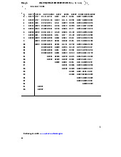
Bảng giá trị phân phối thống kê poisson và student môn Xác suất thống kê| Trường Đại học Ngoại Thương
27 14 -
Bảng giá trị quyết định thống kê wilcoxon rank-sum test môn Xác suất thống kê| Trường Đại học Ngoại Thương
29 15 -

Bài 1 Định nghĩa cổ điển về xác suất môn Xác suất thống kê| Trường Đại học Ngoại Thương
26 13 -

Exercises for probability & statistics môn Xác suất thống kê| Trường Đại học Ngoại Thương
26 13 -
Đề thi cuối kỳ lý thuyết môn Xác suất thống kê| Trường Đại học Ngoại Thương
27 14