The Time Value of Money - English Grammar | Học Viện Phụ phụ nữa Việt Nam

C H A P T E R TIME VALUE 4 OFMONEY
L E A R N I N G G O A L S
Discuss the role of time value in finance, the use
Calculate both the future value and the present LG1 LG4
of computational tools, and the basic patterns of
value of a mixed stream of cash flows. cash flow.
Understand the effect that compounding interest LG5
Understand the concepts of future and present
more frequently than annually has on future value LG2
value, their calculation for single amounts, and
and on the effective annual rate of interest.
the relationship of present value to future value.
Describe the procedures involved in (1) determin- LG6
Find the future value and the present value of both
ing deposits to accumulate a future sum, (2) loan LG3
an ordinary annuity and an annuity due, and find
amortization, (3) finding interest or growth rates,
the present value of a perpetuity.
and (4) finding an unknown number of periods.
Across the Disciplines W H Y T H I S C H A P T E R M AT T E R S TO YO U
Accounting: You need to understand time-value-of-money
bursements in a way that will enable the firm to get the greatest
calculations in order to account for certain transactions value from its money.
such as loan amortization, lease payments, and bond interest
Marketing: You need to understand time value of money rates.
because funding for new programs and products must be justi-
Information systems: You need to understand time-value-of-
fied financially using time-value-of-money techniques.
money calculations in order to design systems that optimize the
Operations: You need to understand time value of money firm’s cash flows.
because investments in new equipment, in inventory, and in
Management: You need to understand time-value-of-money
production quantities will be affected by time-value-of-money
calculations so that you can plan cash collections and dis- techniques. 148 LCV IT ALL STARTS WITH TIME (VALUE)
How do managers decide which cus-
tomers offer the highest profit poten-
tial? Should marketing programs focus on
new customer acquisitions? Or is it better
to increase repeat purchases by existing
customers or to implement programs
aimed at specific target markets? Time-value-of-money calculations can be a key part of such
decisions. A technique called lifetime customer valuation (LCV) calculates the value today (pre-
sent value) of profits that new or existing customers are expected to generate in the future. After
comparing the cost to acquire or retain customers to the profit stream from those customers,
managers have the information they need to allocate marketing expenditures accordingly.
In most cases, existing customers warrant the greatest investment. Research shows that
increasing customer retention 5 percent raised the value of the average customer from 25 per-
cent to 95 percent, depending on the industry.
Many dot-com retailers ignored this important finding as they rushed to get to the Web first.
As new companies, they had to spend to attract customers. But in the frenzy of the moment, they
didn’t monitor costs and compare those costs to sales. Their high customer acquisition costs often
exceeded what customers spent at the e-tailers’ Web sites—and the result was often bankruptcy.
Business-to-business (B2B) companies are now joining consumer product companies like
Lexus Motors and credit card issuer MBNA in using LCV. The technique has been updated to
include intangible factors, such as outsourcing potential and partnership quality. Even though
intangible factors complicate the methodology, the underlying principle is the same: Identify the
most profitable clients and allocate more resources to them. “It actually makes a lot of sense,”
says Bob Lento, senior vice president of sales at Convergys, a customer service and billing ser-
vices provider. Which is more valuable and deserves more of the firm’s resources—a company
with whom Convergys does $20 million in business each year, with no expectation of growing that
business, or one with current business of $10 million that might develop into a $100-million client?
Convergys’s management instituted an LCV program several years ago to answer this question.
After engaging in a trial-and-error process to refine its formula, Convergys chose to include tradi-
tional LCV items such as repeat business and whether the customer bases purchasing decisions
solely on cost. Then it factors in such intangibles as the level within the customer company of a
salesperson’s contact (higher is better) and whether the customer perceives Convergys as a
strategic partner or a commodity service provider (strategic is better).
Thanks to LCV, Convergys’s Customer Management Group increased its operating income
by winning new business from old customers. The firm’s CFO, Steve Rolls, believes in LCV. “This
long-term view of customers gives us a much better picture of what we’re going after,” he says. 149 150 PART 2 Important Financial Concepts LG1
4.1 The Role of Time Value in Finance
Financial managers and investors are always confronted with opportunities to
earn positive rates of return on their funds, whether through investment in
attractive projects or in interest-bearing securities or deposits. Therefore, the tim- Hint The time value of
ing of cash outflows and inflows has important economic consequences, which money is one of the most
financial managers explicitly recognize as the time value of money. Time value is important concepts in finance. Money that the firm has in its
based on the belief that a dollar today is worth more than a dollar that will be possession today is more
received at some future date. We begin our study of time value in finance by con- valuable than future payments
sidering the two views of time value—future value and present value, the compu- because the money it now has can be invested and earn
tational tools used to streamline time value calculations, and the basic patterns of positive returns. cash flow.
Future Value versus Present Value
Financial values and decisions can be assessed by using either future value or pres-
ent value techniques. Although these techniques will result in the same decisions,
they view the decision differently. Future value techniques typically measure cash
flows at the end of a project’s life. Present value techniques measure cash flows at
the start of a project’s life (time zero). Future value is cash you will receive at a
given future date, and present value i
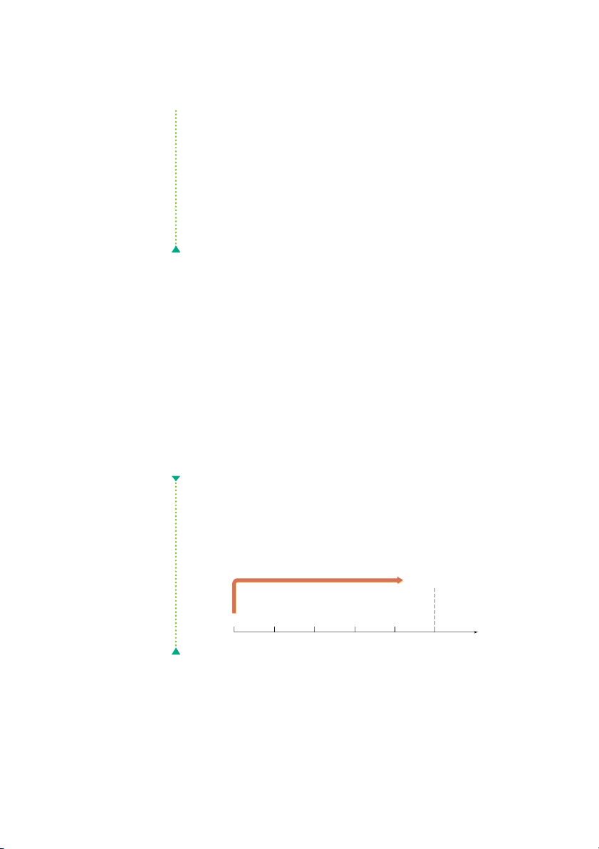
s just like cash in hand today. time line
A time line can be used to depict the cash flows associated with a given
A horizontal line on which time
investment. It is a horizontal line on which time zero appears at the leftmost end
zero appears at the leftmost end
and future periods are marked from left to right. A line covering five periods (in
and future periods are marked
this case, years) is given in Figure 4.1. The cash flow occurring at time zero and
from left to right; can be used to
depict investment cash flows.
that at the end of each year are shown above the line; the negative values repre-
sent cash outflows ($10,000 at time zero) and the positive values represent cash
inflows ($3,000 inflow at the end of year 1, $5,000 inflow at the end of year 2, and so on).
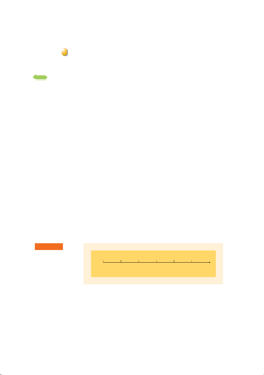
Because money has a time value, all of the cash flows associated with an
investment, such as those in Figure 4.1, must be measured at the same point in
time. Typically, that point is either the end or the beginning of the investment’s
life. The future value technique uses compounding to find the future value of each
cash flow at the end of the investment’s life and then sums these values to find the
investment’s future value. This approach is depicted above the time line in
Figure 4.2. The figure shows that the future value of each cash flow is measured F I G U R E 4 . 1 Time Line –$10,000 $3,000 $5,000 $4,000 $3,000 $2,000 Time line depicting an invest- ment’s cash flows 0 1 2 3 4 5 End of Year CHAPTER 4 Time Value of Money 151 F I G U R E 4 . 2 Compounding Compounding and Discounting Future Time line showing Value compounding to find future value and discounting to find present value –$10,000 $3,000 $5,000 $4,000 $3,000 $2,000 0 1 2 3 4 5 End of Year Present Value Discounting
at the end of the investment’s 5-year life. Alternatively, the present value tech-
nique uses discounting to find the present value of each cash flow at time zero
and then sums these values to find the investment’s value today. Application of
this approach is depicted below the time line in Figure 4.2.
The meaning and mechanics of compounding to find future value and of dis-
counting to find present value are covered in this chapter. Although future value
and present value result in the same decisions, financial managers—because they
make decisions at time zero—tend to rely primarily on present value techniques. Computational Tools
Time-consuming calculations are often involved in finding future and present val-
ues. Although you should understand the concepts and mathematics underlying
these calculations, the application of time value techniques can be streamlined.
We focus on the use of financial tables, hand-held financial calculators, and com-
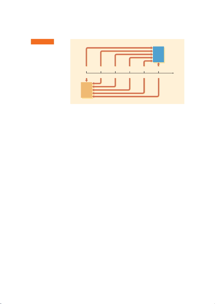
puters and spreadsheets as aids in computation. Financial Tables
Financial tables include various future and present value interest factors that sim-
plify time value calculations. The values shown in these tables are easily devel-
oped from formulas, with various degrees of rounding. The tables are typically
indexed by the interest rate (in columns) and the number of periods (in rows).
Figure 4.3 shows this general layout. The interest factor at a 20 percent interest
rate for 10 years would be found at the intersection of the 20% column and the
10-period row, as shown by the dark blue box. A full set of the four basic finan-
cial tables is included in Appendix A at the end of the book. These tables are
described more fully later in the chapter. 152 PART 2 Important Financial Concepts F I G U R E 4 . 3 Interest Rate Financial Tables Layout and use Period 1% 2% 10% 20% 50% of a financial table 1 2 3 10 X.XXX 20 50 Financial Calculators
Financial calculators also can be used for time value computations. Generally,
financial calculators include numerous preprogrammed financial routines. This
chapter and those that follow show the keystrokes for calculating interest factors
and making other financial computations. For convenience, we use the impor-
tant financial keys, labeled in a fashion consistent with most major financial calculators.
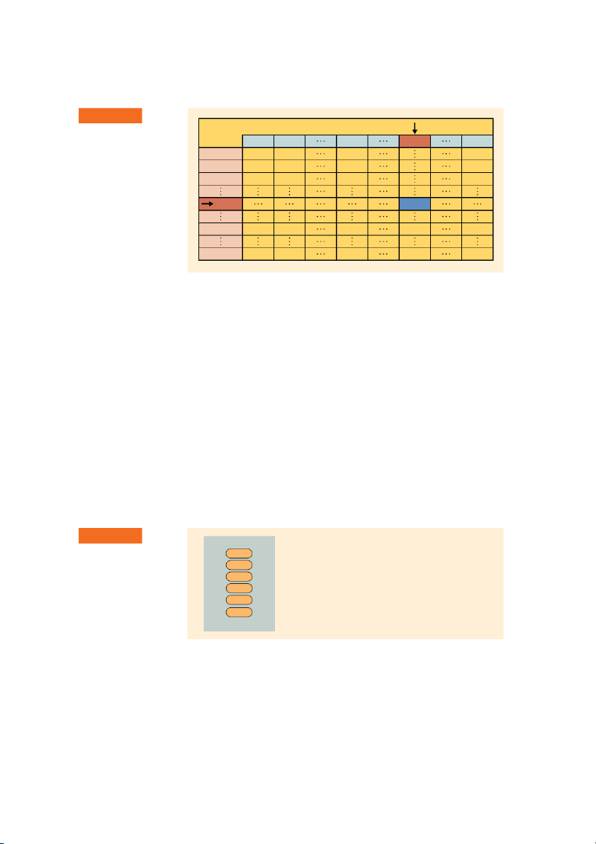
We focus primarily on the keys pictured and defined in Figure 4.4. We typi-
cally use four of the first five keys shown in the left column, along with the com-
pute (CPT) key. One of the four keys represents the unknown value being calcu-
lated. (Occasionally, all five of the keys are used, with one representing the
unknown value.) The keystrokes on some of the more sophisticated calculators
are menu-driven: After you select the appropriate routine, the calculator prompts
you to input each value; on these calculators, a compute key is not needed to
obtain a solution. Regardless, any calculator with the basic future and present
value functions can be used in lieu of financial tables. The keystrokes for other
financial calculators are explained in the reference guides that accompany them.
Once you understand the basic underlying concepts, you probably will want
to use a calculator to streamline routine financial calculations. With a little prac- F I G U R E 4 . 4 N — Number of periods Calculator Keys N Important financial keys I — Interest rate per period I on the typical calculator PV — Present value PV
PMT — Amount of payment (used only for annuities) PMT FV — Future value FV CPT
CPT — Compute key used to initiate financial calculation once all values are input CHAPTER 4 Time Value of Money 153
tice, you can increase both the speed and the accuracy of your financial computa-
tions. Note that because of a calculator’s greater precision, slight differences are
likely to exist between values calculated by using financial tables and those found
with a financial calculator. Remember that conceptual understanding of the
material is the objective. An ability to solve problems with the aid of a calculator
does not necessarily reflect such an understanding, so don’t just settle for answers.
Work with the material until you are sure you also understand the concepts.
Computers and Spreadsheets Hint Anyone familiar with
Like financial calculators, computers and spreadsheets have built-in routines that
electronic spreadsheets, such as
simplify time value calculations. We provide in the text a number of spreadsheet Lotus or Excel, realizes that most of the time-value-of-
solutions that identify the cell entries for calculating time values. The value for money calculations can be done
each variable is entered in a cell in the spreadsheet, and the calculation is pro- expeditiously by using the
grammed using an equation that links the individual cells. If values of the vari- special functions contained in the spreadsheet.
ables are changed, the solution automatically changes as a result of the equation
linking the cells. In the spreadsheet solutions in this book, the equation that
determines the calculation is shown at the bottom of the spreadsheet.
It is important that you become familiar with the use of spreadsheets for sev- eral reasons.
• Spreadsheets go far beyond the computational abilities of calculators. They
offer a host of routines for important financial and statistical relationships.
They perform complex analyses, for example, that evaluate the probabilities
of success and the risks of failure for management decisions.
• Spreadsheets have the ability to program logical decisions. They make it pos-
sible to automate the choice of the best option from among two or more
alternatives. We give several examples of this ability to identify the optimal
selection among alternative investments and to decide what level of credit to extend to customers.
• Spreadsheets display not only the calculated values of solutions but also the
input conditions on which solutions are based. The linkage between a
spreadsheet’s cells makes it possible to do sensitivity analysis—that is, to
evaluate the impacts of changes in conditions on the values of the solutions.
Managers, after all, are seldom interested simply in determining a single
value for a given set of conditions. Conditions change, and managers who are
not prepared to react quickly to take advantage of changes must suffer their consequences.
• Spreadsheets encourage teamwork. They assemble details from different cor-
porate divisions and consolidate them into a firm’s financial statements and
cash budgets. They integrate information from marketing, manufacturing,
and other functional organizations to evaluate capital investments. Laptop
computers provide the portability to transport these abilities and use spread-
sheets wherever one might be—attending an important meeting at a firm’s
headquarters or visiting a distant customer or supplier.
• Spreadsheets enhance learning. Creating spreadsheets promotes one’s under-
standing of a subject. Because spreadsheets are interactive, one gets an 154 PART 2 Important Financial Concepts
immediate response to one’s entries. The interplay between computer and
user becomes a game that many find both enjoyable and instructive.
• Finally, spreadsheets communicate as well as calculate. Their output
includes tables and charts that can be incorporated into reports. They inter-
play with immense databases that corporations use for directing and con-
trolling global operations. They are the nearest thing we have to a universal business language.
The ability to use spreadsheets has become a prime skill for today’s managers.
As the saying goes, “Get aboard the bandwagon, or get run over.” The spreadsheet
solutions we present in this book will help you climb up onto that bandwagon!
Basic Patterns of Cash Flow
The cash flow—both inflows and outflows—of a firm can be described by its gen-
eral pattern. It can be defined as a single amount, an annuity, or a mixed stream.
Single amount: A lump-sum amount either currently held or expected at
some future date. Examples include $1,000 today and $650 to be received at the end of 10 years.
Annuity: A level periodic stream of cash flow. For our purposes, we’ll work
primarily with annual cash flows. Examples include either paying out or
receiving $800 at the end of each of the next 7 years.
Mixed stream: A stream of cash flow that is not an annuity; a stream of
unequal periodic cash flows that reflect no particular pattern. Examples
include the following two cash flow streams A and B. Mixed cash flow stream End of year A B 1 $ 100 ⫺$ 50 2 800 100 3 1,200 80 4 1,200 ⫺ 60 5 1,400 6 300
Note that neither cash flow stream has equal, periodic cash flows and that A
is a 6-year mixed stream and B is a 4-year mixed stream.
In the next three sections of this chapter, we develop the concepts and tech-
niques for finding future and present values of single amounts, annuities, and
mixed streams, respectively. Detailed demonstrations of these cash flow patterns are included. CHAPTER 4 Time Value of Money 155
R e v i e w Q u e s t i o n s 4–1
What is the difference between future value and present value? Which
approach is generally preferred by financial managers? Why? 4–2
Define and differentiate among the three basic patterns of cash flow: (1) a
single amount, (2) an annuity, and (3) a mixed stream. LG2 4.2 Single Amounts
The most basic future value and present value concepts and computations con-
cern single amounts, either present or future amounts. We begin by considering
the future value of present amounts. Then we will use the underlying concepts to
learn how to determine the present value of future amounts. You will see that
although future value is more intuitively appealing, present value is more useful in financial decision making.
Future Value of a Single Amount
Imagine that at age 25 you began making annual purchases of $2,000 of an invest-
ment that earns a guaranteed 5 percent annually. At the end of 40 years, at age 65,
you would have invested a total of $80,000 (40 years ⫻ $2,000 per year). Assum-
ing that all funds remain invested, how much would you have accumulated at the
end of the fortieth year? $100,000? $150,000? $200,000? No, your $80,000
would have grown to $242,000! Why? Because the time value of money allowed
your investments to generate returns that built on each other over the 40 years. compound interest
Interest that is earned on a given
deposit and has become part of
The Concept of Future Value
the principal at the end of a specified period.
We speak of compound interest to indicate that the amount of interest earned on
a given deposit has become part of the principal at the end of a specified period. principal
The term principal refers to the amount of money on which the interest is paid.
The amount of money on which
Annual compounding is the most common type. interest is paid.
The future value of a present amount is found by applying compound interest future value
over a specified period of time. Savings institutions advertise compound interest
The value of a present amount at
returns at a rate of x percent, or x p
ercent interest, compounded annually, semi-
a future date, found by applying
compound interest over a
annually, quarterly, monthly, weekly, daily, or even continuously. The concept of
specified period of time.
future value with annual compounding can be illustrated by a simple example. E X A M P L E
If Fred Moreno places $100 in a savings account paying 8% interest com-
pounded annually, at the end of 1 year he will have $108 in the account—the ini-
tial principal of $100 plus 8% ($8) in interest. The future value at the end of the
first year is calculated by using Equation 4.1:
Future value at end of year 1 ⫽ $100 ⫻ (1 ⫹ 0.08) ⫽ $108 (4.1)
If Fred were to leave this money in the account for another year, he would be
paid interest at the rate of 8% on the new principal of $108. At the end of this 156 PART 2 Important Financial Concepts
second year there would be $116.64 in the account. This amount would represent
the principal at the beginning of year 2 ($108) plus 8% of the $108 ($8.64) in
interest. The future value at the end of the second year is calculated by using Equation 4.2:
Future value at end of year 2 ⫽ $108 ⫻ (1 ⫹ 0.08) (4.2) ⫽ $116.64
Substituting the expression between the equals signs in Equation 4.1 for the
$108 figure in Equation 4.2 gives us Equation 4.3:
Future value at end of year 2 ⫽ $100 ⫻ (1 ⫹ 0.08) ⫻ (1 ⫹ 0.08) (4.3) ⫽ $100 ⫻ (1 ⫹ 0.08)2 ⫽ $116.64
The equations in the preceding example lead to a more general formula for calculating future value.
The Equation for Future Value
The basic relationship in Equation 4.3 can be generalized to find the future value
after any number of periods. We use the following notation for the various inputs:
FVn⫽future value at the end of period n
PV⫽ initial principal, or present value
i ⫽ annual rate of interest paid. (Note: On financial calculators, I is typi-
cally used to represent this rate.)
n ⫽ number of periods (typically years) that the money is left on deposit
The general equation for the future value at the end of period n is FVn⫽PV⫻(1⫹i)n (4.4)
A simple example will illustrate how to apply Equation 4.4. E X A M P L E
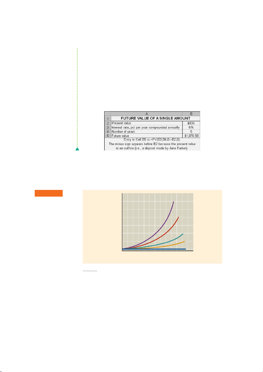
Jane Farber places $800 in a savings account paying 6% interest compounded
annually. She wants to know how much money will be in the account at the end
of 5 years. Substituting PV ⫽ $800, i ⫽ 0.06, and n ⫽ 5 into Equation 4.4 gives
the amount at the end of year 5.
FV5⫽$800⫻(1⫹0.06)5⫽$800⫻(1.338)⫽$1,070.40
This analysis can be depicted on a time line as follows: Time line for future FV5 = $1,070.40 value of a single amount ($800 initial principal, earning 6%, PV = $800 at the end of 5 years) 0 1 2 3 4 5 End of Year CHAPTER 4 Time Value of Money 157
Using Computational Tools to Find Future Value
Solving the equation in the preceding example involves raising 1.06 to the fifth
power. Using a future value interest table or a financial calculator or a computer
and spreadsheet greatly simplifies the calculation. A table that provides values for
(1 ⫹ i)n in Equation 4.4 is included near the back of the book in Appendix Table
future value interest factor
A–1. The value in each cell of the table is called the future value interest factor.
The multiplier used to calculate,
This factor is the multiplier used to calculate, at a specified interest rate, the
at a specified interest rate, the
future value of a present amount as of a given time. The future value interest fac-
future value of a present amount
tor for an initial principal of $1 compounded at i percent for n periods is referred as of a given time. to as FVIFi,n.
Future value interest factor ⫽ FVIFi,n⫽ (1 ⫹ i)n (4.5)
By finding the intersection of the annual interest rate, i, and the appropriate
periods, n, you will find the future value interest factor that is relevant to a par-
ticular problem.1 Using FVIFi,n as the appropriate factor, we can rewrite the gen-
eral equation for future value (Equation 4.4) as follows: FVn⫽PV⫻(FVIFi,n) (4.6)
This expression indicates that to find the future value at the end of period n of an
initial deposit, we have merely to multiply the initial deposit, PV, by the appro-
priate future value interest factor.2 E X A M P L E
In the preceding example, Jane Farber placed $800 in her savings account at 6%
interest compounded annually and wishes to find out how much will be in the account at the end of 5 years. Input Function
Table Use The future value interest factor for an initial principal of $1 on 800 PV
deposit for 5 years at 6% interest compounded annually, FVIF found in 6%, 5yrs, 5 N
Table A–1, is 1.338. Using Equation 4.6, $800 ⫻ 1.338 ⫽ $1,070.40. Therefore, 6 I
the future value of Jane’s deposit at the end of year 5 will be $1,070.40. CPT
Calculator Use3 The financial calculator can be used to calculate the future FV
value directly.4 First punch in $800 and depress PV; next punch in 5 and depress 5 Solution
N; then punch in 6 and depress I (which is equivalent to “i” in our notation) ; 1070.58
finally, to calculate the future value, depress CPT and then FV. The future value
of $1,070.58 should appear on the calculator display as shown at the left. On
1. Although we commonly deal with years rather than periods, financial tables are frequently presented in terms of
periods to provide maximum flexibility.
2. Occasionally, you may want to estimate roughly how long a given sum must earn at a given annual rate to double
the amount. The Rule of 72 is used to make this estimate; dividing the annual rate of interest into 72 results in the
approximate number of periods it will take to double one’s money at the given rate. For example, to double one’s
money at a 10% annual rate of interest will take about 7.2 years (72⫼ 10 ⫽ 7.2). Looking at Table A–1, we can see
that the future value interest factor for 10% and 7 years is slightly below 2 (1.949); this approximation therefore
appears to be reasonably accurate.
3. Many calculators allow the user to set the number of payments per year. Most of these calculators are preset for
monthly payments—12 payments per year. Because we work primarily with annual payments—one payment per
year—it is important to be sure that your calculator is set for one payment per year. And although most calculators
are preset to recognize that all payments occur at the end of the period, it is important to make sure that your calcu-
lator is correctly set on the END mode. Consult the reference guide that accompanies your calculator for instruc-
tions for setting these values.
4. To avoid including previous data in current calculations, always clear all registers of your calculator before
inputting values and making each computation.
5. The known values can be punched into the calculator in any order; the order specified in this as well as other
demonstrations of calculator use included in this text merely reflects convenience and personal preference. 158 PART 2 Important Financial Concepts
many calculators, this value will be preceded by a minus sign (⫺1,070.58). If a
minus sign appears on your calculator, ignore it here as well as in all other “Cal-
culator Use” illustrations in this text.6
Because the calculator is more accurate than the future value factors, which
have been rounded to the nearest 0.001, a slight difference—in this case, $0.18—
will frequently exist between the values found by these alternative methods.
Clearly, the improved accuracy and ease of calculation tend to favor the use of
the calculator. (Note: In future examples of calculator use, we will use only a dis-
play similar to that shown on the preceding page. If you need a reminder of the
procedures involved, go back and review the preceding paragraph.)
Spreadsheet Use The future value of the single amount also can be calculated as
shown on the following Excel spreadsheet.
A Graphical View of Future Value
Remember that we measure future value at the end of the given period. Figure 4.5
illustrates the relationship among various interest rates, the number of periods
interest is earned, and the future value of one dollar. The figure shows that (1) the F I G U R E 4 . 5 20% Future Value 30.00 Relationship Interest rates, time periods, 25.00 and future value of one 15% 20.00 dollar 15.00 10.00 10% alue of One Dollar ($) V 5.00 5% Future 1.00 0% 0
2 4 6 8 10 12 14 16 18 20 22 24 Periods
6. The calculator differentiates inflows from outflows by preceding the outflows with a negative sign. For example,
in the problem just demonstrated, the $800 present value (PV), because it was keyed as a positive number (800), is
considered an inflow or deposit. Therefore, the calculated future value (FV) of ⫺1,070.58 is preceded by a minus
sign to show that it is the resulting outflow or withdrawal. Had the $800 present value been keyed in as a negative
number (⫺800), the future value of $1,070.58 would have been displayed as a positive number (1,070.58). Simply
stated, the cash flows—present value (
PV) and future value (FV)—will have opposite signs. CHAPTER 4 Time Value of Money 159
higher the interest rate, the higher the future value, and (2) the longer the period
of time, the higher the future value. Note that for an interest rate of 0 percent, the
future value always equals the present value ($1.00). But for any interest rate
greater than zero, the future value is greater than the present value of $1.00.
Present Value of a Single Amount
It is often useful to determine the value today of a future amount of money. For
example, how much would I have to deposit today into an account paying 7 per- present value
cent annual interest in order to accumulate $3,000 at the end of 5 years? Present
The current dollar value of a
value is the current dollar value of a future amount—the amount of money that
future amount—the amount of
would have to be invested today at a given interest rate over a specified period to
money that would have to be
equal the future amount. Present value depends largely on the investment oppor-
invested today at a given interest
rate over a specified period to
tunities and the point in time at which the amount is to be received. This section
equal the future amount.
explores the present value of a single amount.
The Concept of Present Value discounting cash flows
The process of finding present values is often referred to as discounting cash
The process of finding present
flows. It is concerned with answering the following question: “If I can earn i
values; the inverse of compound-
percent on my money, what is the most I would be willing to pay now for an ing interest.
opportunity to receive FVn dollars n periods from today?”
This process is actually the inverse of compounding interest. Instead of find-
ing the future value of present dollars invested at a given rate, discounting deter-
mines the present value of a future amount, assuming an opportunity to earn a
certain return on the money. This annual rate of return is variously referred to as
the discount rate, required return, cost of capital, and opportunity cost.7 These
terms will be used interchangeably in this text. E X A M P L E
Paul Shorter has an opportunity to receive $300 one year from now. If he can
earn 6% on his investments in the normal course of events, what is the most he
should pay now for this opportunity? To answer this question, Paul must deter-
mine how many dollars he would have to invest at 6% today to have $300 one
year from now. Letting PV equal this unknown amount and using the same nota-
tion as in the future value discussion, we have PV⫻ (1 ⫹ 0.06) ⫽ $300 (4.7)
Solving Equation 4.7 for PV gives us Equation 4.8: $300 PV⫽ ᎏᎏ (4.8) (1 ⫹ 0.06) ⫽ $283.02
The value today (“present value”) of $300 received one year from today,
given an opportunity cost of 6%, is $283.02. That is, investing $283.02 today at
the 6% opportunity cost would result in $300 at the end of one year.
7. The theoretical underpinning of this “required return” is introduced in Chapter 5 and further refined in subse- quent chapters.