Topic : Predict student performance in secondary education | Tiểu luận môn Tiếng Anh thống kê | Trường Đại học Kinh tế Quốc dân

National Economics University
Topic : Predict student performance in secondary education
Instructor : TS.Nguyen Huyen Trang
List of group members: Tran Minh Thu Nguyen Cong Hoan Le Phan Hoang Giap Pham Thi Van Anh Nguyen Phi Long Nguyen Thuy Trang
Hà Nội, tháng 11/2024 INDEX
I, INTRODUCTION................................................................................................................. 1
1. Rationale..................................................................................................................... 1 2.
Literature Review......................................................................................................... 1 3.
Aims of the Study.........................................................................................................2 4.
Object and Range of Study..........................................................................................2 5.
Research Methods.......................................................................................................4
II. DESCRIPTIVE STATISTICS..............................................................................................5
1. Table........................................................................................................................... 5
1.1. Cross table............................................................................................................... 5
1.2. Frequency table........................................................................................................5
2. Graphs............................................................................................................................ 6
2.1. Barchart.................................................................................................................... 6
2.2. Histogram.................................................................................................................7
2.3. Boxplot..................................................................................................................... 8
2.4. Pie chart...................................................................................................................9
III. INFERENTIAL STATISTICS............................................................................................10 1.
Statistical hypothesis test...........................................................................................10 2.
Linear regression.......................................................................................................11
2.1. Linear regression model.........................................................................................11
2.2. The fit of the model test..........................................................................................11
2.3. Regression analysis...............................................................................................12
IV. CONCLUSION................................................................................................................14 I, INTRODUCTION 1. Rationale
Currently, the state of education faces numerous challenges and opportunities amid a
continuously evolving society. Despite increases in the number of educational programs and
investments in facilities, disparities between urban and rural students remain a serious issue.
Students in urban areas often have access to more learning resources, such as libraries,
learning centers, and extracurricular activities, whereas students in rural areas frequently
struggle to access these services.
Additionally, family-related factors show considerable variation among students,
which is readily observed within each classroom. Parents of high-achieving students tend to
be those with higher educational attainment, often working in fields like education and
healthcare, and typically have a stable financial background as well as strong family and marital support structures.
Furthermore, students who are aware of the importance of studying from an early age,
recognize the value of education, and are effective in time management tend to achieve better
academic results than their peers. Therefore, this research is designed to explore the
relationship between individual, family, and social behavior factors on students' academic
performance, specifically focusing on scores in Mathematics or Portuguese (G3). By
analyzing these factors, this study aims to identify the main predictors of academic success
and offer insights to support the development of more effective educational interventions.
Understanding the factors that influence students' academic performance can also help
educational administrators, teachers, and parents make decisions that better support students
throughout their educational journey, especially in a context where personalized and holistic
education is increasingly prioritized. 2. Literature Review
Cortez and Silva (2008) applied quantitative research methods using data from
students at two Portuguese high schools, Gabriel Pereira and Mousinho da Silveira, to
analyze the relationship between personal, familial, educational conditions, and students'
academic performance. The data were collected and processed using SPSS software, with
variables coded as Nominal, Ordinal, and Scale. Analytical methods included descriptive
statistics, relationship testing among variables, and linear regression modeling to determine
the impact of each factor on students' academic achievements. The dataset included variables
related to demographics (such as gender and age), family background (parental occupation
and education level), living and study conditions (study time, health, and absences), and
students’ grades across terms. The dependent variable is students' academic performance,
measured by term scores: the first-term grade (G1), second-term grade (G2), and final annual
grade (G3). Linear regression analysis was used to assess the impact of these factors on
academic outcomes, identifying those with the greatest influence on student achievement.
The descriptive statistics table provides an overview of the characteristics of 397
students in the sample. The variables include school, gender, age, reasons for choosing the
school, travel time from home to school, and weekly study time. the most noticeable finding
is that over half of the students (50.13%) spend more than 10 hours per day studying. 3 3. Aims of the Study
The primary aim of this study is to analyze the individual, family, and study-related factors
that impact high school students' academic outcomes. By examining characteristics such as
gender, age, parental occupation and education, study time, health status, and absenteeism,
this study seeks to identify the relationships between these factors and students' academic
achievements. Specifically, the research focuses on the relationships between prior term
grades (G1, G2) and final year grades (G3) in Mathematics and Portuguese.
From this, the study also aims to examine other potential factors affecting academic
achievement, ultimately providing recommendations to enhance academic performance.
4. Object and Range of Study
The study sample consists of high school students, with a dataset capturing
information on personal characteristics, family circumstances, and academic outcomes. The
students in this study are enrolled at two schools: Gabriel Pereira and Mousinho da Silveira.
The dataset provides demographic details of the students, such as gender and age, as well as
family-related information, including parental occupation and education level.
In addition, factors related to study conditions and student health are also
documented. Data include information on commuting time to school, weekly study hours,
health status, and the number of absences.
Finally, the dataset includes variables on students' grades across different terms,
specifically the grades for the first term, second term, and final cumulative grade. This data
enables an assessment of students' academic performance based on the various factors recorded within the dataset. VARIABLES Value Label Gender F Female M Male School GP Gabriel Pereira MS Mousinho da Silveira Age from 15 to 22 numeric Address U Urban R Rural famsize LE3 less or equal to 3 GT3 greater than 3 Pstatus T living together A apart Medu 0 None 1 primary education (4th grade) 2 5th to 9th grade 3 secondary education 4 4 higher education Fedu 0 None 1 primary education (4th grade) 2 5th to 9th grade 3 secondary education 4 higher education Mjob Teacher Heath Services at_home Other Fjob Teacher Heath Services At_home Other Reason Home Reputation Course Other Travel time 1 <15 min 2 15 to 30 min 3 30 min. to 1 hour 4 >1 hour Study time 1 <2 hours 2 2 to 5 hours 3 5 to 10 hours 4 >10 hours Freetime 1 Very low 2 low 3 medium 4 High 5 Very high heath 1 Very bad 2 Bad 3 Medium 4 Good 5 Very good absences From 0 to 93 number of school absences 5 5. Research Methods
This study employs a quantitative research method using secondary data from the
research by Cortez and Silva (2008), collected from students. The data includes demographic
factors (such as gender, age, and residence), family background (including parental
occupation, parental education level, and marital status), living and study conditions (study
time, health status, and number of absences), and students' academic performance across terms. 6
II. DESCRIPTIVE STATISTICS 1. Table 1.1. Cross table
Table 2. Mean Statistics on Number of school absences; First, Second and Final period
grade of students by Gender Number
of First period Second period Final period school absences grade grade grade Mean Mean Mean Mean Gender 1 Female 6.22 10.59 10.37 9.95 2 Male 5.12 11.20 11.04 10.86 Total 5.70 10.88 10.69 10.38
Table 2 presents the mean statistics on the number of school absences and grades over
three academic periods, broken down by gender. The data indicates that female students have
an average of 6.22 absences, which is higher than the 5.12 absences reported for male
students. This suggests that female students tend to have more absences than male students.
When it comes to academic performance, male students consistently achieve higher
average grades across all three periods. In the first period, male students have an average
grade of 11.20, while female students have an average of 10.59. This trend continues in the
second period, with male students averaging 11.04, compared to 10.37 for female students.
By the final period, male students maintain a higher average grade of 10.86, while female
students’ average drops slightly to 9.95.
Overall, the table suggests that, despite having fewer absences, male students
generally outperform female students in terms of average grades across all three periods. 1.2. Frequency table
Table 3. Frequency of Reason to choose this school Frequency Percent Valid Cumulative Percent Percent Valid course 146 36.8 36.8 36.8 home 109 27.5 27.5 64.2 other 37 9.3 9.3 73.6 reputation 105 26.4 26.4 100.0 total 397 100.0 100.0
Table 3 provides a breakdown of the reasons students choose this school, using
frequency, percent, valid percent, and cumulative percent to illustrate the distribution of 7
responses. The most common reason for selecting the school is related to the courses offered,
with 146 students (36.8%) choosing this factor. Proximity to home ranks as the second most
cited reason, with 109 students (27.5%), bringing the cumulative percentage to 64.2%.
Reputation is also a significant factor, chosen by 105 students (26.4%), which brings
the cumulative percentage to 100.0%. A smaller group of students, 37 in total (9.3%),
selected other reasons not listed in the main categories.
This analysis shows that the courses offered and the school’s proximity to home are
the primary factors influencing students' decisions to enroll, followed closely by the school’s reputation. 2. Graphs 2.1. Barchart
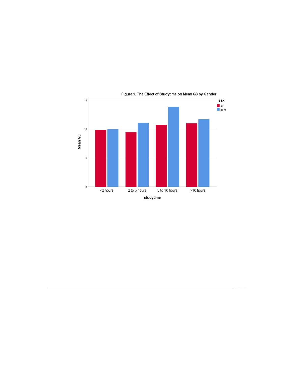
The bar chart compares the average scores in subject G3 between male and female students
based on different study time ranges.
Overall, it is evident that the average score for both genders increases as the study time
becomes longer. However, male students tend to outperform female students when they study for 5 to 10 hours.
For female students, there is a gradual increase in the average score as the study time extends.
The average score for female students who study for less than 2 hours is slightly below 10,
and it increases steadily to just over 11 for those who study for more than 10 hours. 8
In contrast, the average score for male students shows a more significant increase when the
study time is between 2 and 5 hours and 5 to 10 hours. After that, the average score remains
relatively stable. Notably, male students who study for 5 to 10 hours achieve a higher average
score compared to female students in the same study time range.
In conclusion, the bar chart highlights a positive correlation between study time and average
score for both genders. While female students demonstrate a consistent upward trend, male
students experience a more pronounced improvement in their scores when they study for an extended period. 2.2. Histogram
The histogram presents the frequency distribution of the G3 variable.
It can be observed that the data follows a normal distribution pattern, characterized by a bell-
shaped curve. The majority of values cluster around the mean of 10.38, indicating that this is
the most common score. As we move away from the mean in either direction, the frequency of values decreases.
The standard deviation of 4.605 suggests a moderate spread in the data, meaning that values
are distributed fairly evenly around the mean. The bell-shaped curve indicates that most of
the observations fall within one standard deviation of the mean, with fewer observations at the extremes. 9 2.3. Boxplot
The boxplot illustrates the distribution of G3 scores. The vertical axis represents the G3
score, and the horizontal axis shows the range of scores.
The boxplot reveals that the majority of G3 scores fall between approximately 10 and 15. The
median score, indicated by the line within the box, appears to be around 12. The box itself
represents the interquartile range (IQR), which encompasses the middle 50% of the data. The
whiskers extend from the box to the minimum and maximum values, excluding outliers.
There are no outliers present in this dataset, as indicated by the absence of any data points
beyond the whiskers. The distribution appears to be slightly skewed to the right, with a longer
tail on the right side of the boxplot. This suggests that there are more scores towards the
lower end of the range compared to the higher end. 10 2.4. Pie chart
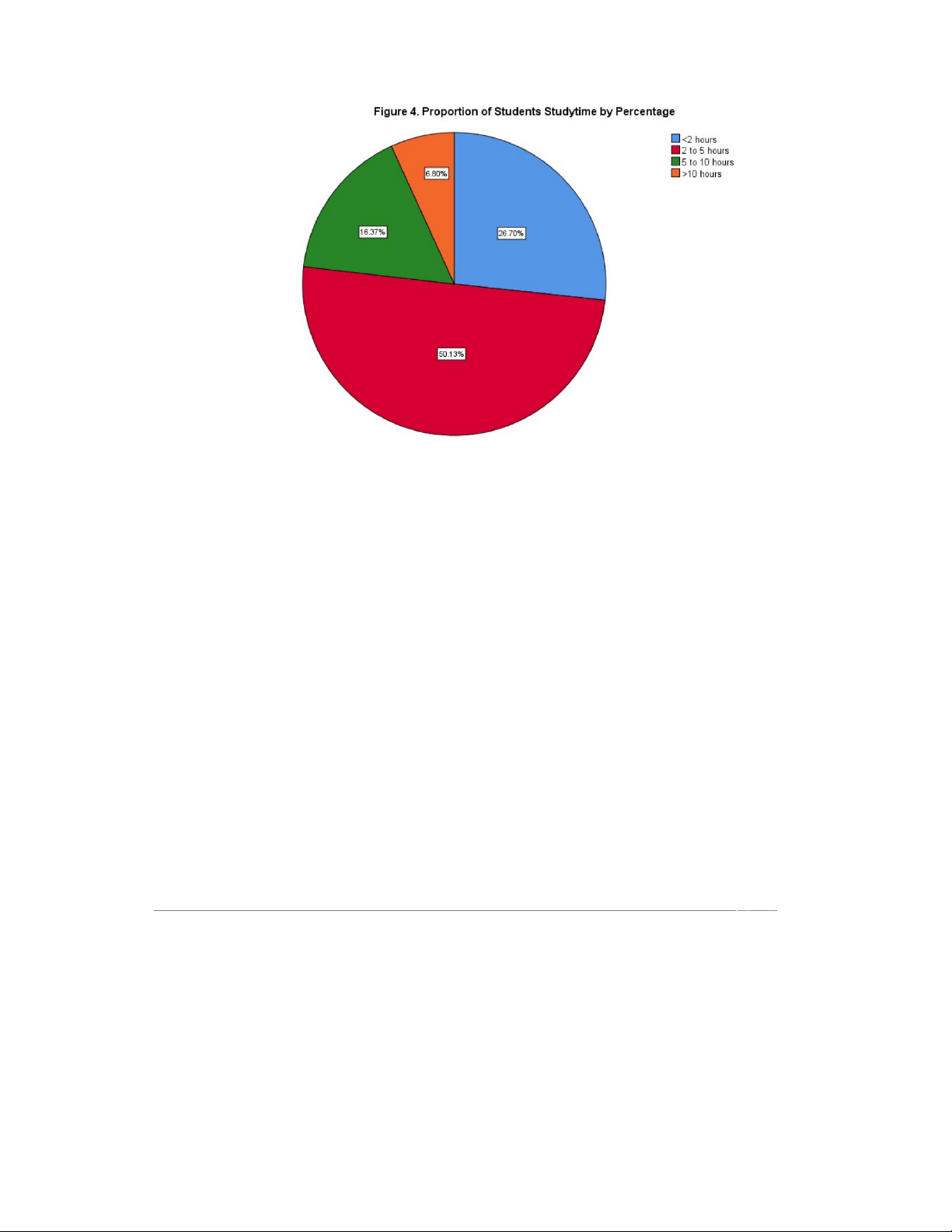
The pie chart illustrates the distribution of students based on their daily study time. It is
evident that a significant proportion of students dedicate a substantial amount of time to their studies.
Specifically, the most noticeable finding is that over half of the students (50.13%) spend
more than 10 hours per day studying. Following closely behind, approximately a quarter of
students (26.70%) study between 5 and 10 hours daily. In contrast, a much smaller
percentage of students study for less than 5 hours, with only 6.80% studying for less than 2 hours.
In conclusion, the data highlights a strong tendency among students to commit a considerable
amount of time to their academic pursuits. 11
III. INFERENTIAL STATISTICS
1. Statistical hypothesis test
According to practical understanding, we can easily see that weekly study time influences
students' grades. To verify this claim, our team conducted a hypothesis test on the differences
in second period grades among students with varying weekly study times.
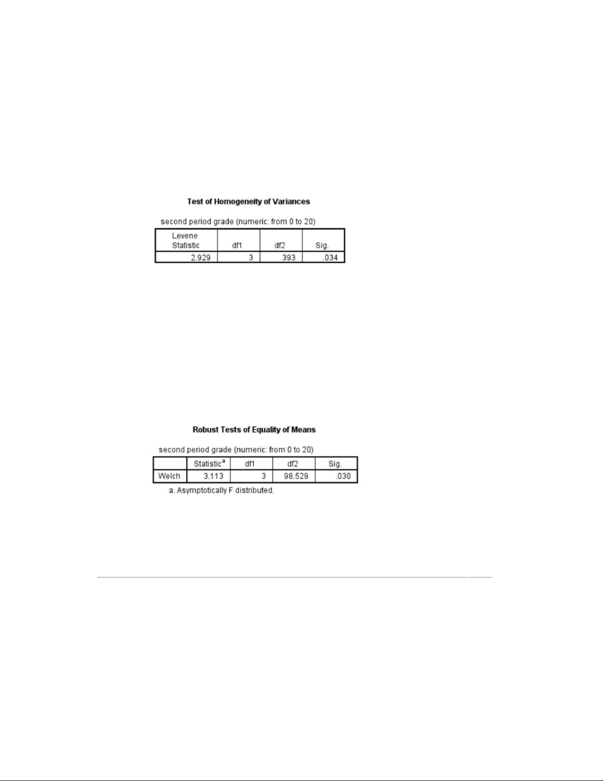
First, we carried out the Levene test to check whether the population variances are equal. Statistical hypothesis:
● H0: The variances of the populations are equal.
● H1: The variances of the populations are different.
After performing the Levene test, we obtained a Sig. value of 0.034, which is less than 0.05.
This result indicates a variance difference between the populations at a 5% significance level.
Therefore, to test for differences in second period grades among groups of students based on
weekly study time, we will proceed with a Welch’s test. Statistical hypothesis:
● H0: There is no difference in grades between students with different weekly study times.
● H1: There are differences in grades between students with different weekly study times. Test statistic: F 12
The results of the Welch test give a Sig. value of 0.03, which is less than 0.05, allowing us to
reject the null hypothesis. We conclude that there is a statistically significant difference
between the populations. Simply put, there are differences in the grades of students who have
different weekly study times at a 5% significance level. In other words, weekly study time is
a factor that affects students' grades. 2. Linear regression
2.1. Linear regression model
* Our team conducted a study on the linear regression model with:
- Dependent variable: Final grade - Independent variable: + First semester grade ( G1) + Second semester grade ( G2 )
+ Number of school absences (N) + Student's age (age)
+ A1( <2 hours), A2( from 2 to 5 hours ), A3( from 5 to 10 hours ) : create these 3 dummy
variables from the numeric variables Study time.
+ B1( very low), B2( low ), B3( medium ), B4( high ) : create these 4 dummy variables from
the numeric variables Freetime.
+ T1( <15min), T2(15 to 30 min), T3(30 min to 1 hour) : create these 3 dummy variables from the traveltime .
+ H1 ( very bad ), H2(bad), H3(medium), H4(good) : create these 4 dummy variables from the health.
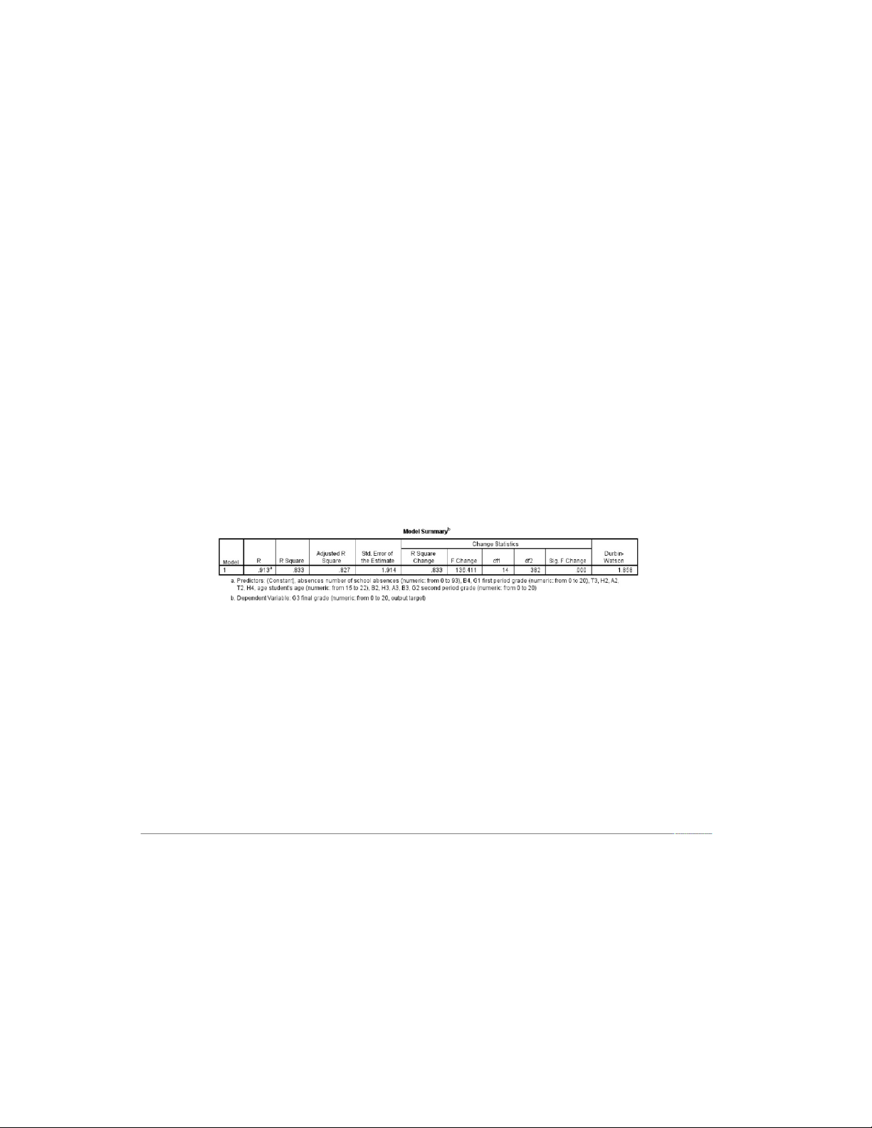
2.2. The fit of the model test
Evaluate the fit of the model.
a. Predictors: (Constant), first semester grade , second semester grade ,A2( from 2 to 5
hours ), A3( from 5 to 10 hours ), B2( low ), B3( medium ), B4( high ), T2(15 to 30 min),
T3(30 min to 1 hour), H2(bad), H3(medium), H4(good), number of school absences, student's age
b. Dependent variable: Final grade
This table shows the R, R-squared, and adjusted R-squared values. The R value provides the
simple correlation and is 0.913, which indicates a relatively high degree correlation. The R-
squared value indicates the overall variability in the dependent variable. The adjusted R-
squared considers the number of predictors in the model and penalizes excessive variables, 13
providing a more accurate measure of the model’s fit, especially with many predictors. The
results in the table show that the adjusted R-squared coefficient = 0.827 means that the model
fit is 82.7% or the dependent factor has been explained by 82.7% of the variation of the
independent factors. Thus, the results of the collected data are explained at a reasonable level
for the model. This shows that the model is suitable.
Test the fit of the regression model:
H0: B0 = B1 = B2 = …. = Bk = 0 (all regression coefficients of variables are equal to 0)
H1: At least 1 regression coefficient can be different from 0
The ANOVA table reports how well the regression equation fits the data. ANOVA analysis
of variance results give Sig. = 0, which is less than 0.05, leading to the conclusion that we can
reject null hypothesis. In short, the regression model is appropriate at 5% significance level. 2.3. Regression analysis
This research conducted regression analysis using the OLS least squares method. Estimate
and test the statistical significance of the regression coefficients
H0: Bn = 0 (estimated regression coefficient is not statistically significant)
H1: Bn ≠ 0 (estimated regression coefficient is statistically significant) 14
The Coefficients table gives us the necessary information to predict the weight from
independent variables and determine if they contribute statistically to the model.
First, we choose Variance Inflation Factor (VIF) to know whether there is multicollinearity in
our regression model. All calculated VIF coefficients are less than 10 , so the model does not
have multicollinearity. Unstandardized Coefficients reflect the expected (linear) change in the
response with each unit change in the predictor. Standardization of the coefficient is done to
answer the question of which of the independent variables have a greater effect on the
dependent variable in a multiple regression analysis where the variables are measured in
different units of measurement. We use values calculated above to present regression equation:
G3 = 1.139 + 0.164G1 + 0.976G2 + 0.06A2 + 0.154A3 - 0.039B2 - 0.112B3 + 0.197B4 -
0.649H2 + 0.131H3+ 0.078H4- 0.128T2+ 0.11T3 - 0.204age+ 0.043N
Of the 14 variables included in the linear regression model, at the 5% significance
level, the test results show that 5 independent variables are statistically significant (Sig.
<0.05). The variables are First semester grade, Second semester grade, student's age, absences number, H2 .
Based on the Standardized Beta Coefficient, we can evaluate the influence of each
factor on the dependent variable. Second semester grade seems to be the strongest influence.
The least influential factor is low’s freetime ( B2)
Specifically, if other factors are the same, a student with a high second semester grade
will be 0.976 points higher than a student with a low second semester grade.Similarly,
students with low’s freetime will score 0.039 points lower than students with high freetime.
This can be explained by the remaining busy time students can spend on studying.
Those in poor health had an impact on their final grades, which were 0.649 points
lower than those in better health.
Age also affects students' results. Statistics show that high age will reduce the score
by 0.204 points compared to low age. Finally, the number of absences of students also affects the final grade of students. IV. CONCLUSION
After analyzing the data, evaluating the variables, and performing hypothesis testing
and regression on the survey response dataset, we can draw several important conclusions
about factors related to high school students' academic outcomes at two Portuguese high
schools, Gabriel Pereira and Mousinho da Silveira.
Female students tend to have higher absence rates in classes compared to male
students at both schools. This somewhat affects the scores in all three categories, as male
students consistently achieve higher grades than female students. Notably, more than half of
the students spend over 10 hours each day studying.
There are five main factors that affect high school students' academic results.We can
calculate the influence level of each factor to the score of them.
Second semester grade(G2) is the factor which has the biggest effect on their outcomes,
followed by the first semester grade(G1) and the number of school absences. 15 16 17