Two sample hypothesis testing solutions môn Xác suất thống kê| Trường Đại học Ngoại Thương

Exercises 8 - Solutions Two Sample Hypothesis Testing
1. Test the hypothesis that the average SAT math scores from students in California
and New York are different. A sample of 45 students from California had an
average score of 552, whereas a sample of 38 New York students had an average
score of 530. Assume the population standard deviations for California and New
York students are 105 and 114 respectively.
a. Test at the  = 0.05 level.
b. Find the p-value for these samples. Answers a. 0 : 1 2 H  =  1 : 1 2 H    Where:
 = the mean SAT scores of California students.
 = the mean SAT scores of New York students.
We can also express the hypothesis as: 0 H : 1 −2 = 0 1 H : 1 −2  0
We are given the following information: n X  Californian Students 45 552 105 New York Students 38 530 114
Let’s test this hypothesis at the  = 0.05 level.
We know that we have a two-tailed test since the alternative hypothesis is 1
H : 1 −2  0 .
Since 1 and 2 are known, and the sample sizes taken are both greater than 29, we can use the following formulas. Z = Z 2= Then we can find 9 . 1 6from the normal tables.  % 5 . 2 1 We use the equation: 2 2 1   2  = + n x − x 1 n 2 1 2 2 105 2 114 = +  1=2 x −x 24 2 . 28 45 38
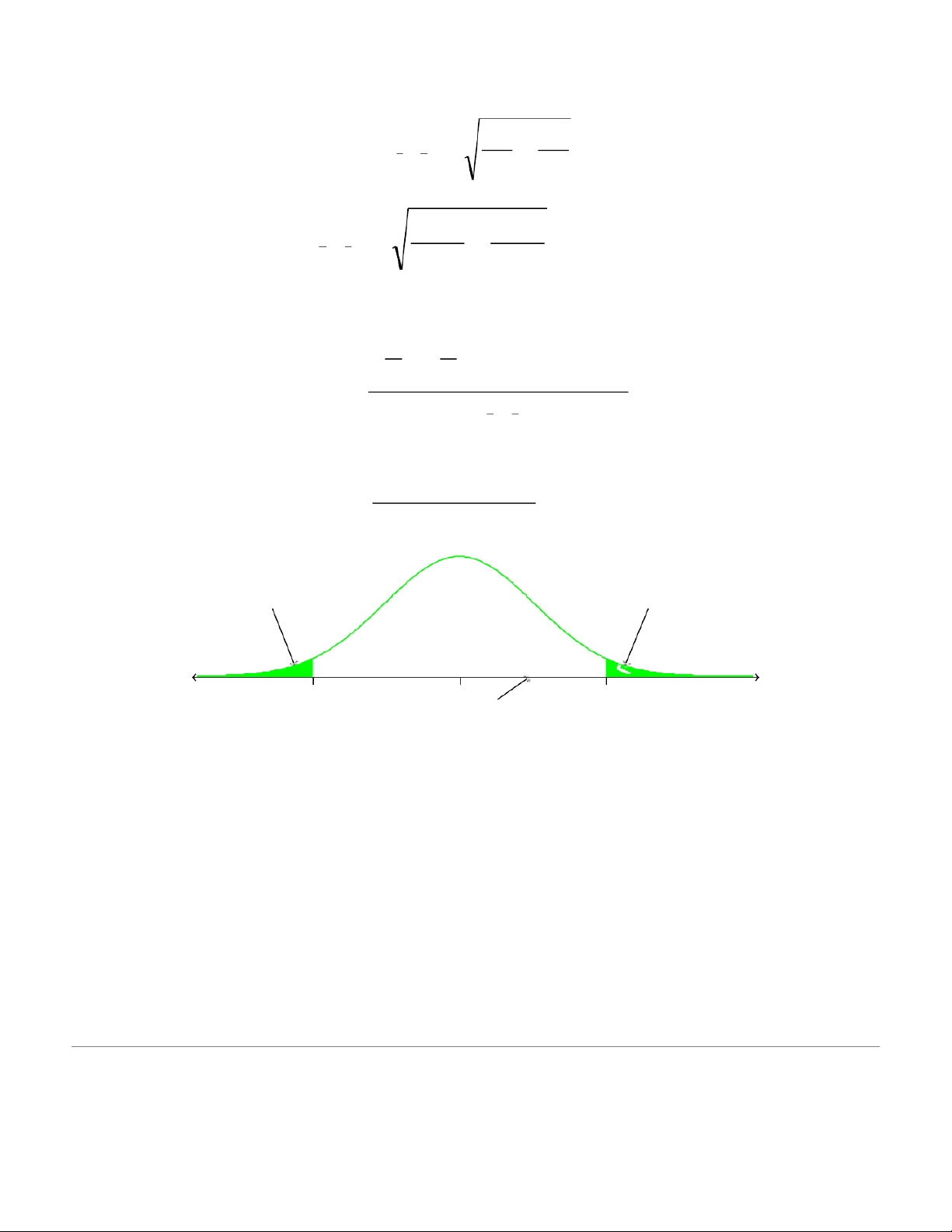
We can now calculate the test statistic, for this two sample test, in standardized form using: 1 2 1 ( X 2 X − )− ( −  ) H0 Z =  x1− x 2 For this example: 5 ( 5 = 2− 53 ) 0 − 0 Z = 9 . 0 08 24 2 . 28 Reject Ho Reject Ho Do NOT reject Ho z –1.96 0 1.96 0.908
Here we do not reject H0 . We conclude that there is not enough evidence to support a
difference between the two states. 2
b. Find the p-value for these samples. Do NOT r 18.14% 31.86% 18.14% z –0.908 0 0.908
The p-value is the sum of the green areas i.e. 18.14% + 18.14% = 36.28% 3
2. A company tracks satisfaction scores based on customer feedback from individual
stores on a scale from 0 to 100. The following data represents the customer scores from Store 1 and Store 2. Store1 : 90 87 93 75 88 96 90 82 95 97 78
sample mean = 88.3, sample standard deviation=7.30 Store 2: 82 85 90 74 80 89 75 81 93 75
sample mean = 82.4, sample standard deviation=6.74
Assume population standard deviations are equal but unknown and that the population is
normally distributed. Test the hypotheses H0:  =  vs. H1: ≠ 
H0:  ≤  vs. H1:  > 
H0:  ≥  vs. H1:  <  Using  = 0.10. 4 a. H 0 : 1 = 2 H 1 : 1   2 Where:
 = the mean satisfaction scores of store 1.
 = the mean satisfaction scores of store 2.
We can also express the hypothesis as: − 0 = 1H : 2  0 − 1  1H : 2  0
We are given the following information: n X s Store 1 11 88.3 7.30 Store 2 10 82.4 6.74
Let’s test this hypothesis at the  = 0.10 level.
We know that we have a two-tailed test since the alternative hypothesis − 1 is  1H : 2  0 .
Since 1 and 2 are not known, and the sample sizes taken are both less than 29, we can use the following formulas.
Even though we do not actually know 1 or 2, we are assuming that they are equal.
Under these conditions we first calculate the pooled estimate of the standard
deviation using the following: (n − ) 12s + (n − ) 1 2 s 1 1 2 2 n Sp =n + − 1 2 2
Putting in the numbers gives: = 2 = 1 ( 12− 3 . 7 ) 1 0 + 1 ( 0− . 6 ) 1 74 941 7 . 48 S = p . 7 04 11+ 10− 2 19
We now approximate the standard error using: 5 1 1 n =  x x + − Sp 1 ˆ n 2 1 2 1 1 1 1 = + T
=his leads to + ˆ 1x 2=x Sp 0 . 7 4 0 . 3 8 n hours −n 1 2 11 10
We can now calculate the t –score for our test statistic: 1 2 1 ( X 2 X − )− ( −  )H 0 t = ˆ  1 x − x2 For this example: 8 ( 8 = 3 . − 82 ) 4 . − 0 t = 9 . 1 18 0 . 3 8
We must now find our cut off, or critical t-score for the “Do Not Reject H0” region.
To look up this value in the t-tables we must first determine the number of degrees of freedom. This is found from: n + 1 n − 2 2
In our case this is equal to 11 + 10 2 = – 19.
The critical t-score from the t-tables is 1.729. Remember that we have a two-tailed test
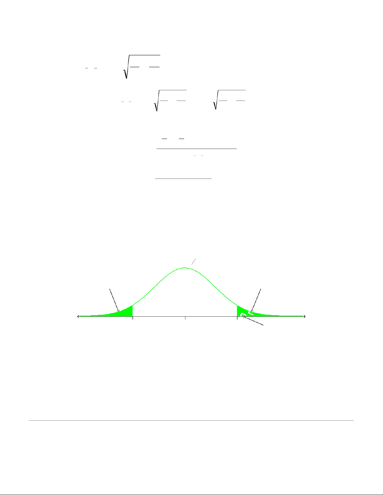
with  = 0.10 and 19 degrees of freedom nt n . ( = 2 19 1 = + 2 t −  % 5 7 . 1 29 ). 2 Reject Ho Reject Ho Do NOT reject Ho –1.729 0 z 1.729 1.918
Here we reject H0 . We may conclude that based on our two samples and the 10% level of
significance we believe that a difference exists between customer satisfaction between the two stores. 6 b. H 0 : 1  2 H1 : 1  2 Where:
 = the mean satisfaction scores of store 1.
 = the mean satisfaction scores of store 2.
We can also express the hypothesis as: − 0  1H : 2  0 − 1  1H : 2  0
We are given the following information: n X s Store 1 11 88.3 7.30 Store 2 10 82.4 6.74
Let’s test this hypothesis at the  = 0.10 level.
We know that we have a one-tail test with the rejection region to the right,since the alternative hypothe − sis i 1 s  1H : 2  0 .
Since 1 and 2 are not known, and the sample sizes taken are both less than 29, we can use the following formulas.
Even though we do not actually know 1 or 2, we are assuming that they are equal.
Under these conditions we first calculate the pooled estimate of the standard
deviation using the following: (n − ) 12s + (n − ) 1 2 s 1 1 2 2 n Sp =n + − 2 1 2
Putting in the numbers gives: = 2 = 1 ( 12− 3 . 7 ) 1 0 + 1 ( 0− . 6 ) 1 74 941 7 . 48 S = p . 7 04 11+ 10− 2 19
We now approximate the standard error using: 7 1 1 n =  x x + − S 1 ˆ n 2 p 1 2 1 1 1 1 = + T
=his leads to + ˆ 1x 2 =x Sp 0 . 7 4 0 . 3 8 n hours −n 11 10 1 2
We can now calculate the t –score for our test statistic: 1 2 1 ( X 2 X − )− ( −  )H 0 t = ˆ  1 x − x2 For this example: 8 ( 8 = 3 . − 82 ) 4 . − 0 t = 9 . 1 18 0 . 3 8
We must now find our cut off, or critical t-score for the “Do Not Reject H0” region.
To look up this value in the t-tables we must first determine the number of degrees of freedom. This is found from: n + 1 n − 2 2
In our case this is equal to 11 + 10 2 = – 19.
The critical t-score from the t-tables is 1.328. Remember that we have a one-tailed test
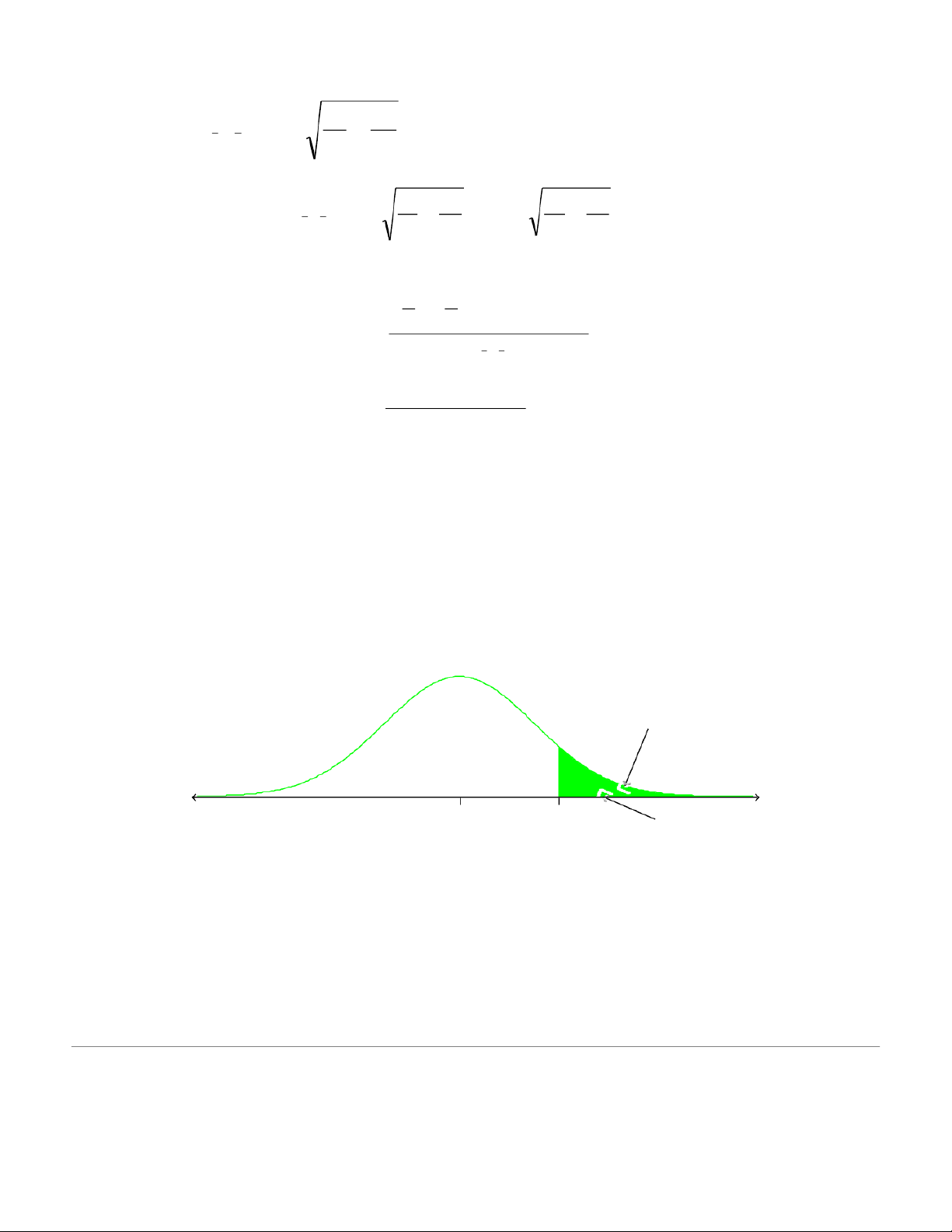
with  = 0.10 and 19 degrees of freedom nt n. ( = 2 19 1 = + 2  t − 1 % 0 3 . 1 28 ). Reject Ho Do NOT reject Ho 0 z 1.328 1.918
Here we reject H0 . We may conclude that based on our two samples and the 10% level of
significance we believe that customer satisfaction is greater at store 1 than store 2. 8 c. H 0 : 1   2  H1 :1  2 Where:
 = the mean satisfaction scores of store 1.
 = the mean satisfaction scores of store 2.
We can also express the hypothesis as: − 0  1H : 2  0 − 1  1H : 2  0
We are given the following information: n X s Store 1 11 88.3 7.30 Store 2 10 82.4 6.74
Let’s test this hypothesis at the  = 0.10 level.
We know that we have a one-tail test with the rejection region to the left, since the alternative hypothe − sis i 1 s  1H : 2   0 .
Since 1 and 2 are not known, and the sample sizes taken are both less than 29, we can use the following formulas.
Even though we do not actually know 1 or 2, we are assuming that they are equal.
Under these conditions we first calculate the pooled estimate of the standard
deviation using the following: (n − ) 12s + (n − ) 1 2 s 1 1 2 2 n Sp =n + − 1 2 2
Putting in the numbers gives: = 2 = 1 ( 12− 3 . 7 ) 1 0 + 1 ( 0− . 6 ) 1 74 941 7 . 48 S = p . 7 04 11+ 10− 2 19
We now approximate the standard error using: 9 1 1 n =  x x + − S 1 ˆ n 2 p 1 2 1 1 1 1 = + T
=his leads to + ˆ 1x 2 =x 0 . 7 4 0 . 3 8 n Sp hours −n 1 2 11 10
We can now calculate the t –score for our test statistic: 1 2 1 ( X 2 X − )− ( −  )H 0 t = ˆ  1 x − x2 For this example: 8 ( 8 = 3 . − 82 ) 4 . − 0 t = 9 . 1 18 0 . 3 8
We must now find our cut off, or critical t-score for the “Do Not Reject H0” region.
To look up this value in the t-tables we must first determine the number of degrees of freedom. This is found from: n + 1 n − 2 2
In our case this is equal to 11 + 10 2 = – 19.
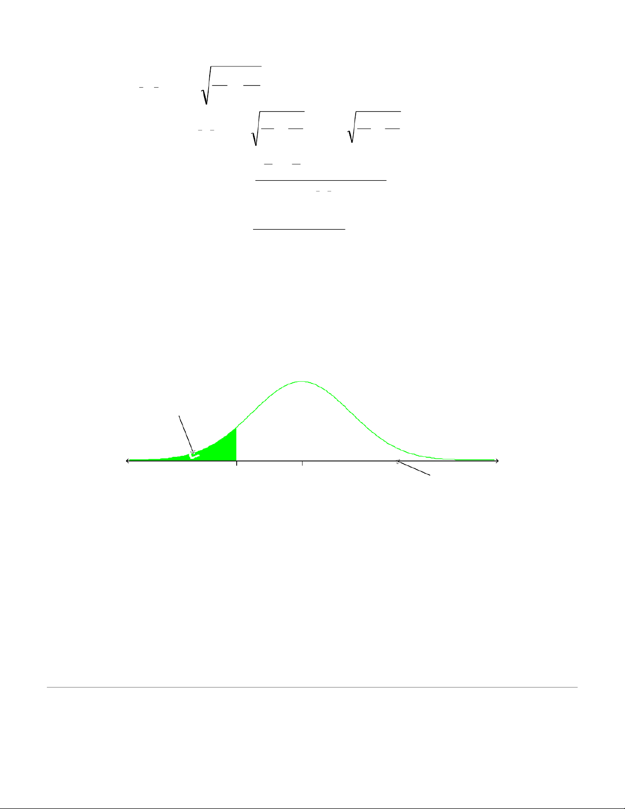
The critical t-score from the t-tables is -1.328. Remember that we have a one-tailed test with  = 0.10 and 19 de nt n grees of − + t f−reedom = . ( − 2 19 1 = −2  1 % 0 3 . 1 28 ). Reject Ho Do NOT reject Ho –1.328 1.918 0 z
Here we do not reject H0 . We may conclude that based on our two samples and the 10%
level of significance we believe that customer satisfaction is at least as great at store 1 compared to store 2.
3. Re-do question 2, but this time assume the population standard deviations are unequal and unknown. a. H 0 : 1 = 2 10 H1 : 1  2 Where:
 = the mean satisfaction scores of store 1.
 = the mean satisfaction scores of store 2.
We can also express the hypothesis as: − 0 = 1H : 2  0 − 1  1H : 2  0
We are given the following information: n X s Store 1 11 88.3 7.30 Store 2 10 82.4 6.74
Let’s test this hypothesis at the  = 0.10 level.
We know that we have a two-tailed test since the alternative hypothesis − 1 is  1H : 2  0 .
Since 1 and 2 are not known, and the sample sizes taken are both less than 29, we can use the following formulas.
Even though we do not actually know 1 or 2, we are assuming that they are not equal.
We can now calculate the t-test statistic, for this two sample test, in standardized form: 1 2 1 ( X 2 X − )− ( −  )H 0 t = where ˆ  1x−x2 2 2 1 s s2 . 7 3 2 7 . 6 2 2 = + ˆ  1x=2x 0 . 3 7 −n 1 n 2 11 10
For this example the test statistic becomes: 8 ( =. 8 3− 82 4 . )− 0 t = 9 . 1 2 0 . 3 7 Degrees of freedom: 11 2 + 2 2 s s  1 2    1 n n2   2 2   2 2    s  1    s  2     n     n 
  1   +   2    n − 1  1 2  n −1          Since 2s 3. 7 2 2 0 s 7 . 6 2 4 = 1= 8 . 4 4 = 2= . 4 n 11 54 n 10 1 2 In our case this will be: Degrees of freedom (4 8 . 4+ 5 . 4 ) 4 2= 18 9 . 9599721  ( 8 . 4 ) 4 2  ( 5 . 4 ) 4 2  +   10     9  
The degrees of freedom must be expressed as an integer, so we round this figure up to the
next whole number which is 19.
We now find the critical t-score by looking at the t-tables, remembering that we have a
two- tailed test with  = 0.10 and we have 19 degrees of freedom. The critical t-score is 1.729. ( 2 19 nt n = 1 = + 2 t −  % 5 7 . 1 29 ) 2 Reject Ho Reject Ho Do NOT reject Ho –1.729 0 z 1.729 1.92
Here we can see that we will reject H . 0 12 b. H 0 : 1   2  H1 : 1  2 Where:
 = the mean satisfaction scores of store 1.
 = the mean satisfaction scores of store 2.
We can also express the hypothesis as: − 0  1H : 2  0 − 1  1H : 2  0
We are given the following information: n X s Store 1 11 88.3 7.30 Store 2 10 82.4 6.74
Let’s test this hypothesis at the  = 0.10 level.
We know that we have a one-tail test with the rejection region to the right, since the alternative hypothe − sis i 1 s  1H : 2  0 .
Since 1 and 2 are not known, and the sample sizes taken are both less than 29, we can use the following formulas.
Even though we do not actually know 1 or 2, we are assuming that they are not equal.
We can now calculate the t-test statistic, for this two sample test, in standardized form: 1 2 1 ( X 2 X − )− ( −  )H 0 t = ˆ  1x−x2 where 2 2 s1 s2 3 . 7 0 2 7 . 6 22 = + ˆ  1= 2 x x 0 . 3 7 −n 1 n 2 11 10
For this example the test statistic becomes: 8 ( 8 = 3 . − 82 4 . )− 0 t = 9 . 1 2 0 . 3 7 13 2 + 2 2 s s  1 2    1 n n2  Degrees of freedom:  2 2   2 2    s  1    s  2     n     n 
  1   +   2    n − 1  1 2  n −1          Since 2 s 3 . 7 2 0 2 s 7 . 6 2 4 = 1= 8 . 4 4 = 2= 5 . 4 4 n 11 n 10 1 2 In our case this will be: Degrees of freedom (4 8 . 4+ 5 . 4 ) 4 2= 18 9 . 9599721  ( 8 . 4 ) 4 2  ( 5 . 4 ) 4 2  +  10   9     
The degrees of freedom must be expressed as an integer, so we round this figure up to the
next whole number which is 19.
We now find the critical t-score by looking at the t-tables, remembering that we have a
one tail test with  = 0.10 and we have 19 degrees of freedom. The critical t-score is 1.328. ( nt = n 2 19 1 = + 2 t −  1 % 0 3 . 1 28 ). Reject Ho Do NOT reject Ho 0 z 1.328 1.92 14
Here we can see that we will reject H . 0 c. H 0 : 1   2  H1 :1  2 Where:
 = the mean satisfaction scores of store 1.
 = the mean satisfaction scores of store 2.
We can also express the hypothesis as: − 0  1H : 2  0 − 1  1H : 2  0
We are given the following information: n X s Store 1 11 88.3 7.30 Store 2 10 82.4 6.74
Let’s test this hypothesis at the  = 0.10 level.
We know that we have a one-tail test with the rejection region to the left, since the alternative hypothe − sis i 1 s  1H : 2   0 .
Since 1 and 2 are not known, and the sample sizes taken are both less than 29, we can use the following formulas.
Even though we do not actually know 1 or 2, we are assuming that they are not equal.
We can now calculate the t-test statistic, for this two sample test, in standardized form: 1 2 1 ( X 2 X − )− ( −  )H 0 t = where ˆ  1x−x2 2 2 s1 s2 3 . 7 0 2 7 . 6 22 = + ˆ  1= 2 x x 0 . 3 7 −n 1 n 2 11 10
For this example the test statistic becomes: 8 ( 8 = 3 . − 82 4 . )− 0 t = 9 . 1 2 0 . 3 7 15 2 + 2 2 s s  1 2    1 n n2  Degrees of freedom:  2 2   2 2    s  1    s  2     n     n 
  1   +   2    n − 1  1 2  n −1          Since 2s 3. 7 2 2 0 s 7 . 6 2 4 = 1= 8 . 4 4 = 2= . 4 n 11 54 n 10 1 2 In our case this will be: Degrees of freedom (4 8 . 4+ 5 . 4 ) 4 2= 18 9 . 9599721  ( 8 . 4 ) 4 2  ( 5 . 4 ) 4 2  +   10     9  
The degrees of freedom must be expressed as an integer, so we round this figure up to the
next whole number which is 19.
We now find the critical t-score by looking at the t-tables, remembering that we have a
one tail test with  = 0.10 and we have 19 degrees of freedom. The critical t-score is nt n − + t − -1.328. ( = − 2 19 1 = −2  1 % 0 3 . 1 28 ). Reject Ho Do NOT reject Ho –1.328 1.92 0 z
Here we can see that we will not reject H0 . 16
4. Bank of America’s Consumer Spending Survey collected data on annual credit card charges
in seven different categories of expenditures: transportation, groceries, dining out,
household expenses, home furnishings, apparel and entertainment. Using data from a
sample of 42 credit card accounts, assume that each account was used to identify the
annual credit card charges for groceries (population 1) and the annual credit card charges
for dining out(population 2). Using the difference data, the sample mean was ,
and the sample standard deviation was .
a. Formulate the null and alternative hypotheses to test for no difference between
the population mean credit card charges for groceries and the population mean
credit card charges for dining out.
b. Use a 0.05 level of significance. Can you conclude that the population means differ? c. What is the p-value?
d. Which category, groceries or dining out, has a higher population mean annual credit card charge? Solutions
a. =population mean grocery expenditures
=population mean dining-out expenditures b.
df= n-1=41. Can either use p-value or critical point to draw conclusion. Critical
point will be 2.02 from t table.
The conclusion is that there is a difference between the annual population mean
expenditures for groceries and for dining out. c. p-value is approximately 0
d. Groceries have a higher mean annual expenditure by an estimated $850. 17
5. Airline travelers often choose which airport to fly from based on flight cost. Cost data (in
dollars) for a sample of flights to eight cities from Dayton Ohio, and Louisville, Kentucky,
were collected to help determine which of the two airports was more costly to fly from. A
researcher argued that it is significantly more costly to fly out of Dayton than Louisville.
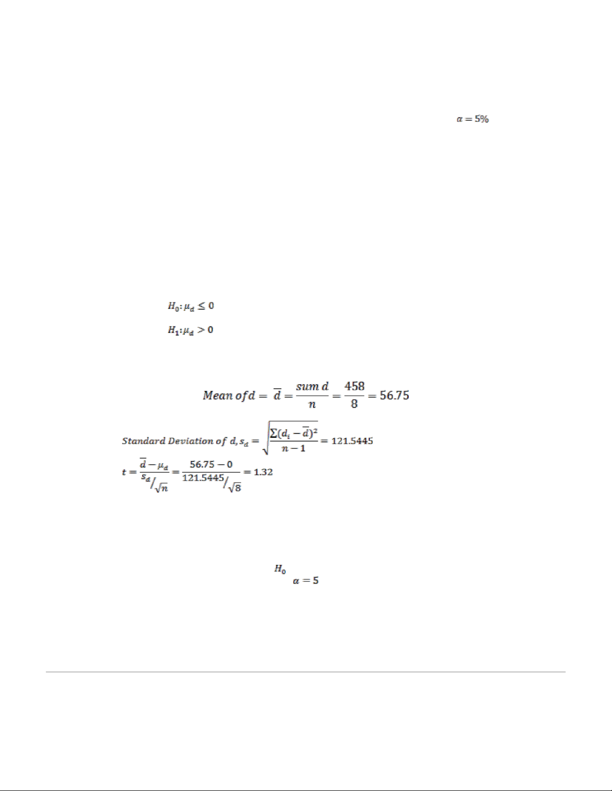
Use the sample data to see whether they support the researcher’s argument, Use as the level of significance. Destination Dayton Louisville Chicago-O’Hare $319 $142 Grand Rapids, Michigan 192 213 Portland, Oregon 503 317 Atlanta, Georgia 256 387 Seattle, Washington 339 317 South Bend, Indiana 379 167 Miami, Florida 268 273 Dallas-Ft. Worth, Texas 288 274 Answer a.
Differences are 177, -21, 186, -131, 22, 212, -5, 14 df=n-1=7
Using t table, p-value is greater than 0.10
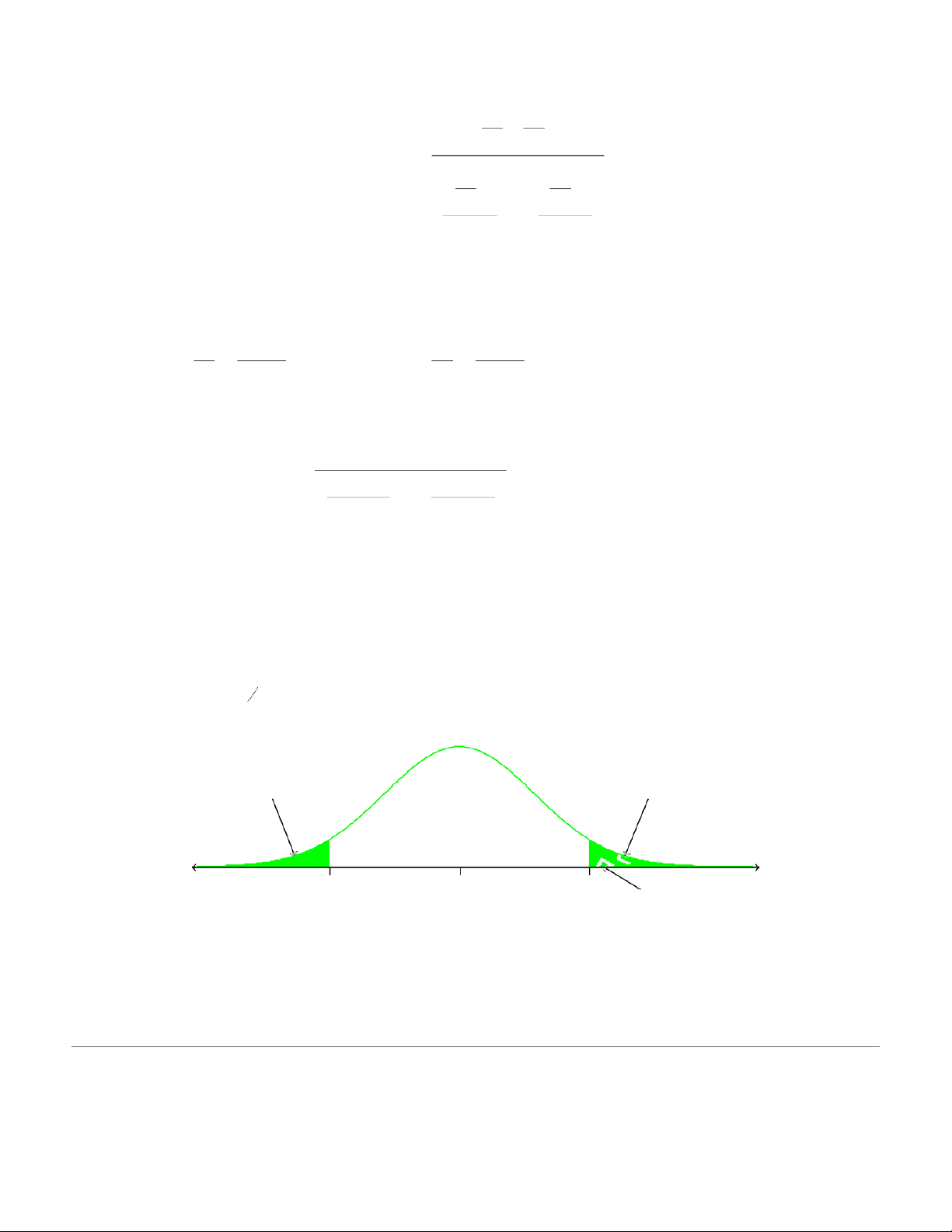
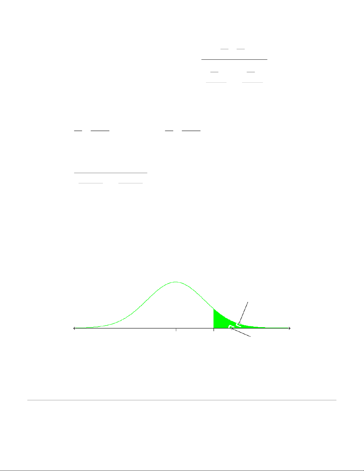
Exact p-value corresponding to t=1.32 is 0.1142
Since p-value> 0.10 we do not reject . We cannot conclude that airfares from Dayton
are higher than those from Louisville at a %. Level of significance. 18
6. In recent years, a growing array of entertainment options competes for consumer time. By
2004, cable television and radio surpassed broadcast television, recorded music, and the
daily newspaper to become the two entertainment media with the greatest usage.
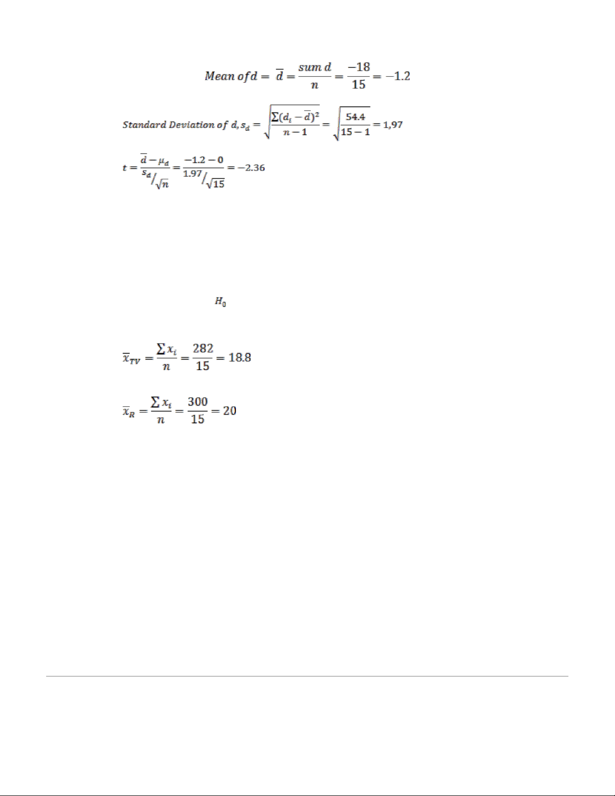
Researchers used a sample of 15 individuals and collected data on the hours per week
spent watching cable television and hours per week spent listening to radio. Individual Television Radio 1 22 25 2 8 10 3 25 29 4 22 19 5 12 13 6 26 28 7 22 23 8 19 21 9 21 21 10 23 23 11 14 15 12 14 18 13 14 17 14 16 15 15 24 23 18.8 5,4142 5,4248
a. Use a 0.05 level of significance and test for a difference between the population mean
usage for cable television and radio. b. What is the p-value?
c. What is the sample mean number of hours per week spent listening to radio?
d. Which medium has greater usage? Answers a.
Use difference data: -3, -2, -4, 3, -1, -2, -1, -2, 0, 0, -1, -4, -3, 1, 1 19 d.f. = n-1=14
Using t table, area is between 0.01 0.025
Two-tail p-value is between 0.02 and 0.05
b. Exact p-value corresponding to t=-2.36 is 0.0333
p-value ≤ 0.05, reject . Conclude that there is a difference between the population
mean weekly usage for the two media. c.
Hours per week for cable television Hours per week for radio
d. So radio has greater usage. 20