An outlook towards hydrogen supply chainnetworks in 2050 — Design of novel fuelinfrastructures in Germany
An outlook towards hydrogen supply chainnetworks in 2050 — Design of novel fuelinfrastructures in Germany. Tài liệu được sưu tầm giúp bạn tham khảo, ôn tập và đạt kết quả cao. Mời bạn đọc đón xem.
Môn: Tài liệu Tổng hợp 3.6 K tài liệu
Trường: Tài liệu khác 3.9 K tài liệu
Tác giả:


Preview text:
Chemical Engineering Research and Design 1 3 4 ( 2 0 1 8 ) 90–103
Contents lists available at ScienceDirect
Chemical Engineering Research and Design
j o u r n a l h o m e p a g e : w w w . e l s e v i e r . c o m / l o c a t e / c h e r d
An outlook towards hydrogen supply chain
networks in 2050 — Design of novel fuel
infrastructures in Germany
Anton Ochoa Bique ∗, Edwin Zondervan
Laboratory of Process Systems Engineering, Department of Production Engineering, Universität Bremen, Leobener
Str. 6, 28359 Bremen, Germany a r t i c l e i n f o a b s t r a c t Article history:
This work provides a comprehensive investigation of the feasibility of hydrogen as trans- Received 30 August 2017
portation fuel from a supply chain point of view. It introduces an approach for the
Received in revised form 20 March
identification the best hydrogen infrastructure pathways making decision of primary energy 2018
source, production, storage and distribution networks to aid the target of greenhouse gas Accepted 23 March 2018
emissions reduction in Germany. The minimization of the total hydrogen supply chain (HSC) Available online 3 April 2018
network cost for Germany in 2030 and 2050 years is the objective of this study. The model
presented in this paper is expanded to take into account water electrolysis technology driven Keywords:
by solar and wind energy. Two scenarios are evaluated, including a full range of technologies Hydrogen supply chain design
and “green” technologies using only renewable resources. The resulting model is a mixed Fuel infrastructures
integer linear program (MILP) that is solved with the Advanced Integrated Multidimensional
Mixed integer linear programming
Modeling System (AIMMS). The results show that renewable energy as a power source has Germany
the potential to replace common used fossil fuel in the near future even though currently AIMMS
coal gasification technology is the still the dominant technology.
© 2018 Institution of Chemical Engineers. Published by Elsevier B.V. All rights reserved. 1. Introduction
and biomass based production of energy and chemicals is strongly
supported by governments (Schill, 2014). For example, the German
Up till now, fossil fuels, which include natural gas, oil, and coal are
government decided to completely phase out nuclear energy by 2022
the primary energy sources for transportation, electricity, and residen-
(Pregger et al., 2013) and replace it with renewable energy production.
tial services. Based on a report by the International Energy Agency
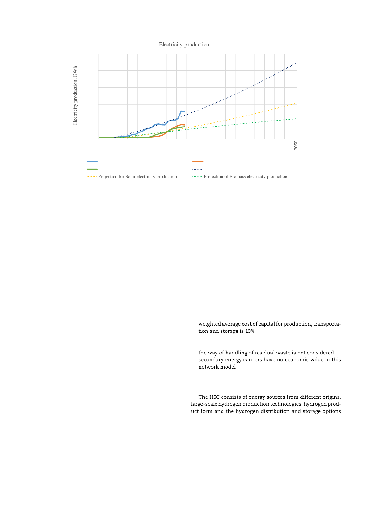
The largest part of renewable power will come from solar and wind as
(IEA) and the U.S. EIA, the global energy demand will grow with 30% in
shown in Fig. 1. Electric power from wind mills increases its contribu-
2040 (International Energy Agency (IEA), 2016; U.S. Energy Information
tion by 225 TWh in 2050, which is 39% of the final produced energy; solar
Administration, 2017). This means a progressively growing fuel con-
contributes 17%, at 100 TWh per year, while biomass reaches 60 TWh
sumption in the near future i.e. greenhouse gas emissions such as per year.
carbon dioxide also increase. Fossil fuel is a nonrenewable energy
While biomass as a raw material might be stored for a long period
source. The depletion time for fossil fuel is estimated to be around
of time, wind and solar are more difficult to handle. As battery sys-
100 years, where oil and gas will be exhausted earlier than coal (Shafiee
tems do currently not have enough capacity and storage of electricity
and Topal, 2009). Moreover, due to increasing fuel consumption, cause
is very expensive, the developments in new long-term storage technol-
of concern is the fast rise of CO
ogy is one of the main challenges. Industrial key players, like Siemens
2 level, now already exceeding 400 ppm
level and, left unmitigated, can possibly double in 100 years to 800 ppm
currently work on a new type of energy storage system based on hydro- (CO2.earth, n.d.).
gen production (Siemens, n.d.). The main idea is that excess energy
Due to the increasing demand of electric energy and a decreas-
from renewable energy sources can be converted into hydrogen from
ing amount of fossil fuel sources, the development of solar-, wind-
water by electrolysis, which is a non-toxic source of energy to con-
∗ Corresponding author.
E-mail address: antochoa@uni-bremen.de (A. Ochoa Bique).
https://doi.org/10.1016/j.cherd.2018.03.037
0263-8762/© 2018 Institution of Chemical Engineers. Published by Elsevier B.V. All rights reserved.
Chemical Engineering Research and Design 1 3 4 ( 2 0 1 8 ) 90–103 91 Nomenclature TC
Daily distribution cost [$ d−1] TCCf ,t
Capital cost of transport mode t for distribution Indices
hydrogen in the form f [$] e Type of energy source Total Total cost of HSC network [$] f Type of hydrogen physical form g
Grid points, each grid point represents German Integer variables state
NPFp,f ,g Number of production facility p generating p
Type of hydrogen production facility
hydrogen in from f at grid point g s Type of storage facility NSF
of storage facility s holding hydrogen s,f ,g Number t Type of transportation mode
in the form f at grid point g
NTFg,g,f ,t The number of transport mode t used for Abbreviation
hydrogen distribution in the form f from g to CH Compressed-gaseous hydrogen g FCEV Fuel cell electric vehicle PNg
Population at the grid point g HSC Hydrogen supply chain IEA International Energy Agency Parameters LH Liquid hydrogen AvCon
Average of household energy consumption USEIA
U.S. Energy Information Administration [kWh d1] AvD
The average distance travelled by personal car Continuous variable [km y1]
EESAve,g Amount of available energy source e in the grid AvT
The average amount of personal car per 1000
point g, which is used to satisfy energy demand people
in grid point g [kWh d−1] AFp
Annual factor for the facility p [%]
EESNe,g,g The flowrate of the supplied energy source e AFs
Annual factor for the s storage facility s [%]
from neighboring grid point g to grid point g, AFt
Annual factor for the transport mode t [%]
which is used to satisfy energy demand in grid Disg,g
Distance between grid points [km] point g [kWh d−1]
Disg,g,t Distance between grid points depending of type
ESAve,g Amount of available energy source e in the grid of transport [km] point g [unit e d−1]
ESCoste Energy source e price in year y, generated locally ESC
Total cost for the energy source consumed for [$ unit−1 e] hydrogen production [$ d−1] ESDise Delivery price for energy source e ESDg
Daily energy source demand [kWh d−1] [$ unit−1 km−1] HDg
Hydrogen demand by grid point [kg d−1]
ESICoste Energy source e import price [$ unit−1]
HFg,g,t,f Hydrogen flowrate in the form f from grid point FE
The fuel economy [kg H2 km−1]
g to g via transportation mode t [kg d−1] FPt
Fuel price for transport mode t [$ l−1] HHEDg
Total energy demand in the grid point g
MaxPCapp/MinPCapp Max/min production capacity for [kWh d−1]
hydrogen production facility p [kg d−1] HPg,f
Hydrogen generation in the form f at grid point OP Operating period [d y−1] g [kg d−1] SCaps,f
Capacity of storage facility s for holding hydro- HPp,g,f
Amount of produced hydrogen in the produc- gen in the from f [kg]
tion facility p in the form f at grid point g [kg d−1] PC
Daily production costs [$ d−1] Greek letters PCC
Production capital cost [$ d−1] ˛
ratio between energy sources e consump- e,p The
PESAve,g Amount of available energy source e in the grid
tion to produce 1 kg [unit e kg1 H 2]
point g, which is used to satisfy energy source FCEVs penetration rate [%]
demand for hydrogen production [unit e d−1]
Is total product storage period [d]
PESIme,g,g Flowrate of imported energy source e from
neighboring grid point g to grid point g, which
is used to satisfy energy source demand for
hydrogen production [unit e d−1]
sumers allowing a greater energy security and flexibility. As soon as PESNe
there is energy shortage, hydrogen might be used in different appli-
,g,g Flowrate supplying energy source e from
neighboring grid point g to grid point g
cations such as power generation, domestic and industrial services, [unit e d−1]
navigation and space (Hake et al., 2006). However, hydrogen is not a
naturally occurring fuel of mineral origin; it can be produced from POC
Production operating cost [$ d−1]
both renewable and non-renewable resources: from coal and biomass PCC p,f
Capital cost of facility p, producing hydrogen in
gasification, the reforming of natural gas, from water electrolysis, form f [$]
photo-electrolysis, water-splitting thermochemical cycle, photobio- POCp,f
Hydrogen production operating cost in form f
logical production, and high temperature decomposition. Moreover,
at facility p [$ kg−1]
hydrogen generation is only a part of the hydrogen production net- SC
The total hydrogen storage cost [$]
work, which can be defined as a supply chain consisting of several SCCp,f
Capital cost for storage facility s holding hydro-
components (such as production, storage and distribution). For each gen in the form f [$]
of these stages a wide range of potential technological options exist. SOCp
Due to increasing demand for energy, the development of sustainable ,f
Operating cost to store 1 kg of hydrogen in the
from f inside of storage facility s [$ kg−1 d−1]
and environmental friendly concepts such as the HSC should be devel-
oped to replace non-sustainable alternatives to meet the global need for 92
Chemical Engineering Research and Design 1 3 4 ( 2 0 1 8 ) 90–103 250000 200000 150000 100000 50000 0 1990 1993 1996 1999 2002 2005 2008 2011 2014 2017 2020 2023 2026 2029 2032 2035 2038 2041 2044 2047 Year Wind electricity production Solar electricity prodution Biomass
Projection for Wind electricity production
Fig. 1 – Projection of energy generation.
energy (Ball et al., 2007). The work of Hugo et al. (2005) takes all possible
develop and describe the model, setup a case study and interpret and
hydrogen alternatives for the design of an optimal hydrogen infras- discuss the results obtained.
tructure in Germany in to consideration. However, their model does
not include energy sources distribution and the ability of centralized 2.
Network description and problem
hydrogen storage to satisfy the local demand. A study of Almansoori statement
investigated a number of strategic decisions for hydrogen fuel pro-
duction and hydrogen delivery networks in Germany at large-scale 2.1.
Problem statement
considering emission targets and carbon tax as a part of the model for-
mulation for 2030 (Almansoori and Betancourt-Torcat, 2016). The main
Given are the location and capacity of energy source suppliers,
objective in that study was to satisfy the hydrogen demand which was
determined by a fuel cell electric vehicles (FCEVs) penetration of 10%
capital and operating costs for a large-scale hydrogen pro-
of the overal passenger transport. The results showed that liquefied
duction, transportation and storage facilities of the network,
hydrogen production by coal gasification facilities at large-scale and under the conditions that:
delivery via railway tank cars results in the best HSC network struc-
ture. Large-size facilities showed benefit compared to a small-scale
1. location of storage facilities is fixed;
facility since large facilities have a high energy efficiency. Renewable
2. all natural gas is imported (despite a national 12% produc-
energy such as wind and solar were not included in that study due to tion of natural gas);
technical- and economical hurdles such as expenses of electricity price
3. weighted average cost of capital for production, transporta-
for water electrolysis technology and size-independent electrolyzer tion and storage is 10%;
efficiency. The rate of renewable energy consumption to generate a unit
of hydrogen for both sizes of electrolysis facility is identical as the elec-
4. electricity is the main energy source to power rail freight
trolyzer efficiency is independent of the facility size. A similar model
transport (International Union of Railways, 2012);
was developed for the United Kingdom (Almansoori and Shah, 2012).
5. the way of handling of residual waste is not considered;
The objective was the minimization of the cost of the network consider-
6. secondary energy carriers have no economic value in this
ing capital- and operating costs. The results showed the dominance of network model;
steam methane reforming technology. Large-scale electrolysis facilities
7. electricity price based on industrial electricity price for
were not considered due to a size-independent electrolyzer efficiency Germany. that was mentioned before.
The aim of this paper is to develop and evaluate an optimization
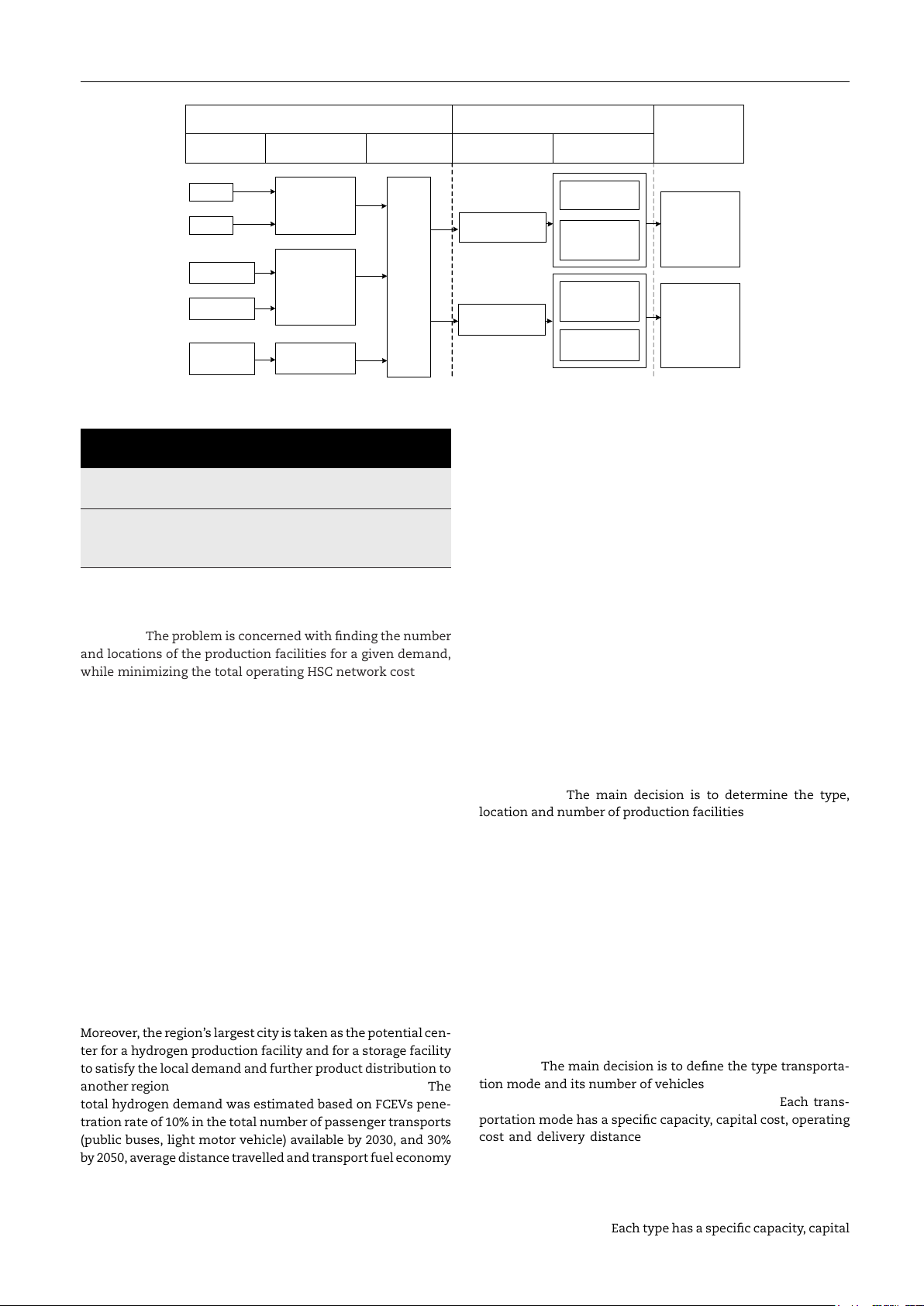
The HSC consists of energy sources from different origins,
model that can be used to solve a HSC network design problem forecast-
ing in 2030 and 2050 years while considering a full range of local factors
large-scale hydrogen production technologies, hydrogen prod-
such as (i) energy sources distribution for hydrogen production, (ii) local
uct form and the hydrogen distribution and storage options
hydrogen demand and (iii) distribution between the place of hydrogen
(Fig. 2). Five types of energy sources are considered: wind-
production and hydrogen demand. The model is used to define the
and solar energy, biomass, natural gas and coal. In addition,
procurement of energy sources from the supplier, the type, the num-
four types of hydrogen production technologies are included
ber and the location of a production facility, the hydrogen production
into the model: steam methane reforming, coal gasifica-
form and the delivery of hydrogen to consumers. The logistics of renew-
tion, biomass gasification and water electrolysis. As hydrogen
able sources is also included into the model by accounting for personal
might be generated by different production technologies, it
needs such as household energy and hydrogen based fuel consump-
may be transported into two forms (i.e. liquid or gaseous),
tion. In addition, this work also considers environmental influences.
which determines the transportation mode that will be used.
Moreover, all techno-economic parameters were collected for 2015 and
were assumed stay same as for the reference years. The German land-
The liquid form (LH) could be stored in super-insulated spher-
scape provides an important case study as Germany has an immense
ical tanks and be distributed via two types of transportation
potential to develop a sustainable hydrogen infrastructure (Hake et al.,
modes: by railway tank car or via tanker truck. Gaseous hydro-
2006). In the following sections we will define the problem statement,
gen (CH) could be stored into pressurized cylindrical vessels
Chemical Engineering Research and Design 1 3 4 ( 2 0 1 8 ) 90–103 93 PRODUCTION DISTRIBUTION STORAGE ENERGY OPTION SOURCE TYPE OF PLANT PRODUCT PRODUCT FORM DISTRIBUTION MODE Wind Tube trailer Electrolysis Pressurized Solar Compression Railway tube Cylindrical car vessels Biomass H2 Gasification Railway tank Coal car Liquefaction Super-insulated Spherical tanks Tanker truck Steam Natural gas reforming
Fig. 2 – Structure of the hydrogen supply and delivery chain.
in Fig. 4), the household energy demand was estimated over
Table 1 – Parameters used for total hydrogen demand calculation in Germany. time. Parameter Passenger transport system in Germany 2015 2.2.2. Primary energy sources
Hydrogen can be produced from different sources such as Number 45,046,564
water, natural gas, biomass and coal. This resource availability
Average distance travelled (km y−1) 13,000
at each grid point plays an important role in defining the type Fuel economy (kg H 2 km−1) 0.018
and location of production technologies (see Appendix F). In
addition, the main problem of a domestic production facility is
and be distributed via railway tube car or tube trailer. Each
concerned with finding an appropriate energy source supplier.
facility of the HSC includes: a technological option, a capacity,
There are three opportunities related with the energy source
a location. The problem is concerned with finding the number
consumption from (i) a domestic grid point or (ii) supply from
and locations of the production facilities for a given demand,
neighboring grid points or (iii) import from abroad.
while minimizing the total operating HSC network cost. 2.2.3. Hydrogen production 2.2.
Model description
Considering that hydrogen is not a naturally occurring fuel
of mineral origin, different production technologies, including
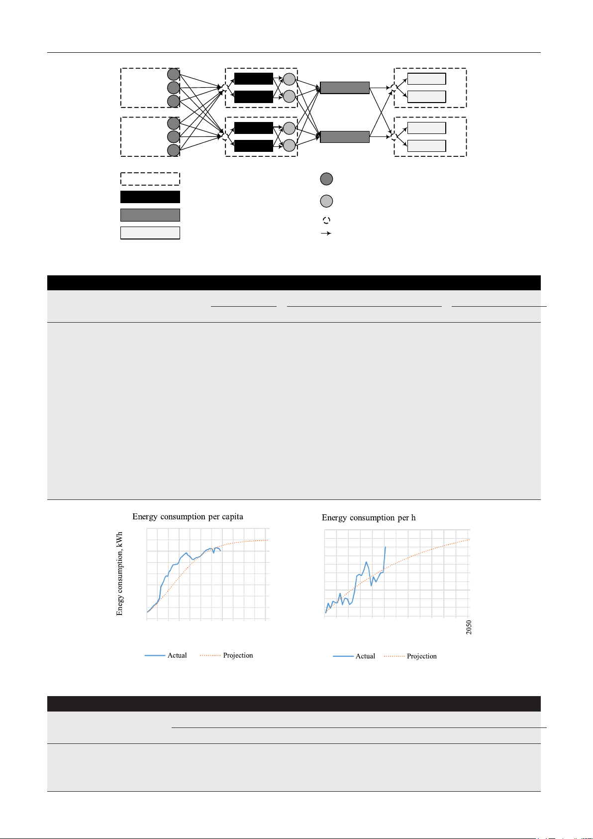
In Fig. 3 the superstructure of HSC model is shown (Hugo
steam methane reforming, coal gasification, biomass gasifica-
et al., 2005). The superstructure includes all the possible
tion and water electrolysis, are generally used to generate it.
connections between the model components. Ultimately, an
Each alternative has fixed capital and operational costs (see
optimization algorithm is used to search for the best strategy
Appendix A). The main decision is to determine the type,
to minimize the costs of the HSC network. The superstructure
location and number of production facilities. Each facility car-
consists a set of grid points (g, each grid point represents a
ries out large-scale hydrogen production (960 t per day) (see
German state), energy sources (e), different transportation (t) Table 3).
modes, different hydrogen production-(p) and storage (s) facil-
ities. The transportation modes are used to distribute different 2.2.4. Hydrogen physical form
types of hydrogen (f) from production facility to storage facil-
Hydrogen can be carried in two physical forms: liquid and
ity. In the following subsections, each component of the HSC
gaseous. Each form is distributed by different transportation
model will be described in more detail.
modes and might be stored in special storage facilities. The
hydrogen form plays an important role in defining which 2.2.1. Grid
transportation mode and storage facilities should be used.
In this study, the landscape of Germany is divided into 16 grid
These decisions affect the final costs of the HSC network.
points, each of this grid points represents a German region.
Moreover, the region’s largest city is taken as the potential cen- 2.2.5. Transportation mode
ter for a hydrogen production facility and for a storage facility
The transportation mode is related to the hydrogen form (gas
to satisfy the local demand and further product distribution to
or liquid). The main decision is to define the type transporta-
another region (Almansoori and Betancourt-Torcat, 2016). The
tion mode and its number of vehicles used to deliver the final
total hydrogen demand was estimated based on FCEVs pene-
product from production point to storage point. Each trans-
tration rate of 10% in the total number of passenger transports
portation mode has a specific capacity, capital cost, operating
(public buses, light motor vehicle) available by 2030, and 30%
cost and delivery distance (see Table 4). It is noted that the
by 2050, average distance travelled and transport fuel economy
operating cost is associated with the delivery distance.
(see Table 2) (BM Verkehr Bau und Stadtentwicklung, 2013).
2015 was used as the reference year for the calculations. All 2.2.6. Storage facility
relevant parameters are listed in Table 1. Based on the pro-
The storage facility, just like the transportation mode, is linked
jections of energy consumption from 1960 to 2050 (as shown
to the hydrogen form. Each type has a specific capacity, capital 94
Chemical Engineering Research and Design 1 3 4 ( 2 0 1 8 ) 90–103 Region g Energy source e Production technology type p Hydrogen form f Distribution mode t Combiner Storage facility s Energy/Material flow
Fig. 3 – Model superstructure.
Table 2 – Local energy and hydrogen demand for the 2030 and 2050. Grid points, g German region Population (MM)
Household energy consumption (GWh d−1) Hydrogen demand (t d−1) 2030 2050 2030 2050 2030 2050 1. Baden-Wurttemberg 10.80 10.10 34.20 32.74 380.81 1068.39 2. Bavaria 12.90 12.10 40.85 39.23 454.86 1279.95 3. Berlin 3.70 3.60 11.72 11.67 130.46 380.81 4. Brandenburg 2.30 1.90 7.28 6.16 81.10 200.98 5. Bremen 0.60 0.60 1.90 1.95 21.16 63.47 6. Hamburg 1.80 1.80 5.70 5.84 63.47 190.41 7. Hesse 6.00 5.60 19.00 18.16 211.56 592.37 8. Mecklenburg-Vorpommern 1.40 1.20 4.43 3.89 49.36 126.94 9. Lower Saxony 7.50 6.70 23.75 21.72 264.45 708.73 10. North Rhine-Westphalia 16.90 15.30 53.52 49.60 595.90 1618.45 11. Rhineland-Palatinate 3.80 3.40 12.03 11.02 133.99 359.65 12. Saarland 0.90 0.80 2.85 2.59 31.73 84.62 13. Saxony 3.80 3.30 12.03 10.70 133.99 349.08 14. Saxony-Anhalt 1.90 1.60 6.02 5.19 66.99 169.25 15. Schleswig-Holstein 2.80 2.40 8.87 7.78 98.73 253.87 16. Thuringia 1.90 1.60 6.02 5.19 66.99 169.25 Total 79.00 72.00 250.18 233.42 2785.56 7616.22 ousehold 9000 3600 h 8000 3550 W 7000 3500 , k 3450 on 6000 3400 pti 5000 3350 4000 3300 nsum 3250 3000 3200 gy co 2000 3150 ner 1000 E 3100 0 8 6 4 2 0 8 6 4 2 0 8 0 5 0 5 0 5 0 5 0 5 0 5 196 196 197 198 199 200 200 201 202 203 204 204 199 199 200 200 201 201 202 202 203 203 204 204 Year Year
Fig. 4 – Projection of energy consumption.
Table 3 – Capital and unit production costs of hydrogen production technologies (Simbeck and Chang, 2002). Parameters Facility type Steam reforming Coal gasification Electrolysis Biomass gasification Capacity (kg d−1) 960,000 960,000 960,000 960,000 Product form LH CH LH CH LH CH LH CH Facility capital cost (Mio $) 1082 775 1668 1123 1910 1663 1895 1518
Unit production cost ($ kg−1) 1.55 0.97 1.66 0.95 6.40 5.86 2,19 1,58
Chemical Engineering Research and Design 1 3 4 ( 2 0 1 8 ) 90–103 95
Table 4 – Parameters used to estimate the capital and operating costs of transportation modes (Amos, 1999). Transpiration mode Tanker truck Tube trailer Railway tank car Railway tube car Capacity (kg trip−1) 4082 181 9072 454 Total cost ($) 500.000 250,000 500,000 300,000 Fuel economy (km unit−1a) 2,550 1.133 22.637 Fuel price ($ unit−1a) 1,22 0,05
a Unit for truck and trailer in l, for railway car in kWh.
denotes the ratio between the energy sources e consumption to
Table 5 – Capital and unit storage costs of hydrogen
storage facilities (Almansoori and Shah, 2012).
produce 1 kg of hydrogen in production facility p. The demand
must be covered by local power generation and/or imports Storage type Super-insulated Pressurized
from neighboring grid points as follows: spherical tanks cylindrical vessel Product form LH CH ESD PESAv +PESIm e,g ≤ e,g+ PESN e,g, ∀g (4) g e,g ,g Capacity (kg) 540,000 540,000 Storage capital cost (Mio $) 122 1894 where PESAve
the amount of available energy source e at
Unit storage cost ($ kg−1 d−1) 0,005 0,076 ,g is
grid point g, which is used to satisfy the demand for energy
source e at grid point g, PESNe,g the flowrate supplying
and operating cost (see Table 5). Storage facilities are installed ,g is
energy source e from neighboring grid point g to grid point g,
at each grid point to satisfy the local hydrogen demand. Stor-
and PESIme,g is the flowrate importing energy source e to grid
age facilities could be located next to production plant or away point g. from it.
The price for the energy source consumed in year y is cal- culated as follows: 3. Model formulation ESC = (PESN ESDise Dis +PESAve,g ESCoste
This section represents the model constraints, the compo- e,g ,g g ,g g ,g,e
nents and objective function, resulting in a MILP. +PESIme,g ESICoste) (5) 3.1.
Household energy demand
where ESICoste represents the energy source e import price,
ESCoste denotes the energy source e price, generated locally,
As mentioned earlier, the household’s energy demand by grid
ESDise is the delivery price for energy source e, and Disg ,g is
point was estimated by projections of the German popula-
the distance between grid points.
tion (Statistisches Bundesamt, n.d.) and energy consumption
till 2050. The household energy demand can be calculated as 3.3. Hydrogen demand follows:
The hydrogen demand by grid point can be calculated as fol- HHEDg = PNgAvCon, ∀g (1) lows:
where HHEDg is the total energy demand at grid point g, PNg HD ␥PN AvD FE, ∀g (6)
represents the population at grid point g, AvCon denotes aver- g = g AvT
age of household energy consumption. The demand must be
where represents the FCEVs penetration rate, AvT repre-
covered by local energy sources generation and/or imports
sents the average number of personal cars per 1000 people,
from neighboring grid points as follows:
AvD is the average distance travelled by a personal car, and FE
denotes the fuel economy. The demand must be satisfied by HHED g ≤ e EESAve,g+ EESN , ∀g (2) g e,g ,g
local production and/or import from neighboring grid points as follows: where EESAv
e,g is amount of available energy source e in grid
point g, which is used to satisfy the energy demand in grid HD HP , ∀g (7) point g, and EESN
the flowrate of the supplied energy g ≤ f g,f + t,g HFg,g,t,f e,g,g is
source e from neighboring grid point g to grid point g. Prefer-
ably, the renewable energy source e will be used to satisfy the
where HPg,f represents the hydrogen generation in the form f household energy demand.
at grid point g, and HFg,g,t,f is hydrogen flowrate in the form f
from a neighboring grid point g to g via transportation mode 3.2.
Demand for a certain energy source t.
The demand for a certain energy source must be satisfied to 3.4.
Hydrogen generation
ensure production. The demand for a certain energy source is calculated as follows:
The hydrogen production is described as follows: ESD ∀ g,e = g (3) HPg,f = HPp,g,f, g, f (8) f,p HPp,g,f ˛e,p, ∀e, p
where HPp,g,f denotes the amount of produced hydrogen in
where HPp,g,f , denotes the amount of produced hydrogen in
the production facility p in the form f at grid point g and ˛e,p
the production facility p in the form f at grid point g. The 96
Chemical Engineering Research and Design 1 3 4 ( 2 0 1 8 ) 90–103
hydrogen production rate is constrained by a maximum and
ity s for holding hydrogen in the from f, is total product minimum capacities as follows: storage period.
The total hydrogen storage cost is calculated as follows: MinPCapp NPFp,f,g ≤ HP MaxPCap g, f (9) p,g,f ≤ p NPFp,f,g, ∀p, SCCs,f NSFs,f,g AFs SC = + SOC (HF s,f g,f+ where MaxPCap t,g HFg,g,t,f)
p, MinPCapp is the max/min production capac- f,s,g OP f
ity for hydrogen production facility p, NPF (15) p,f ,g represents
number of installed production technologies p at grid point
g, Each production plant has an associated capital- and oper- where SCCp
the capital cost for storage facility s
ating cost, the total daily production cost is given by: ,f denotes
holding hydrogen in the form f, AFs is annuity factor for the
s storage facility, SOCp,f is the operating cost to store 1 kg of PC = PCC+POC (10)
hydrogen in the form f at storage facility s.
where PCC represents the production capital cost, and POC is 3.7.
Objective function
production operating cost. Each cost factor can be calculated as follows:
The total cost of HSC network is given as follows: PCCp,f NPFp,f,g AFp PC = +HP (11) min Total = PC + TC + SC + ESC (16) p,g,f POCp,f p,f,g OP
The right-hand side of Eq. (16) contains four parts: the costs where PCC
p,f represents the capital cost of facility p, producing
of hydrogen production (PC), transport (TC), storage (SC), and
hydrogen in form f, NPF
p,f ,g denotes the number of production
energy sources (ESC). The objective is to minimize the total
facilities p generating hydrogen in form f at grid point g, AF p
annualized cost finding the combination of network compo-
is an annuity factor for facility p, OP represents the operating
nents to satisfy the local hydrogen demand under the given period, and POC
p,f denotes the hydrogen production cost in
constraints. The model is coded in AIMMS and is solved with
form f at facility p.
CPLEX 12.6.3. The model consists 8922 equations, 3694 contin-
uous variables, and 2241 integer variables. 3.5.
Hydrogen distribution 4. Case study
The product flowrate by transportation mode t from g to g is given as follows:
Almansoori and Betancourt-Torcat (2016) concluded that the
development of a HSC in Germany is economically feasible for HP g,f ≥ ∀g (12) t,g HFg,g,t,f,
the following reasons: there are already 20 hydrogen fueling
stations across country and the government is reaching the
It is noted that the product can only move in one direction
decarbonization target for private transport and reduction of
between grid points. The total distribution cost, calculated as
greenhouse gases of at least 85% by 2050.
the sum of the operating and capital costs, is represented as:
To validate the model, a future HSC scenario analysis for
Germany was performed. The data was collected from the Fed- TCC f,t NTFg,gf,t AFt TC = + NTF
eral Statistical Office of Germany (Statistisches Bundesamt, f,t,g,g OP g,g,f,t Disg,g,t FPt
n.d.), the Fraunhofer Institute (ISE, n.d.) for Solar Energy Sys- (13)
tems ISE, and Almansoori and Betancourt-Torcat (2016).
This work considers two case studies. Each case represents
where TCCf ,t denotes the capital cost of transport mode t for
a design of an HSC network for Germany for 2030 and 2050.
the distribution of hydrogen in form f, NTFg,g the number ,f ,t is
The first case study considers a scenario to satisfy local hydro-
of transport mode t used for the hydrogen distribution in the
gen demand on the HSC by using the whole range of available
form f from g to g, AFt is an annuity factor for transport mode
technologies. The second case considers a “green” scenario, t, Disg,g
the distance between grid points depending ,t denotes
which represents the ability to satisfy local personal needs
on the type of transport, and FPt is the fuel price for trans-
(local household energy demand first and hydrogen based
port mode t. The driver’s wage and maintenance costs are not
fuel demand after using rest of energy sources) by using only included.
renewable sources (see Appendix E). 3.6. Hydrogen storage 5. Results and discussion
The required hydrogen storage is constrained by a maximum 5.1.
Base case scenario
and minimum capacities as follows:
The optimization results show that 3 or 8 large coal gasifica- NSF ≤ HP s,f s,f,g MinSCaps,f f g,f + t,g HFg,g,t,f
tion hydrogen facilities are selected as most economic option (14)
to satisfy hydrogen demand in 2030 and 2050 respectively for ≤ NSF , ∀g
the first scenario (see Appendix B). Coal is one of the main s,f s,f,g MaxSCaps,f
power sources in Germany. Moreover, capital and operating
where NSFs,f ,g denotes the number of storage facility s holding
costs for a coal gasification facility are very low. In energy
hydrogen in form f at grid point g, and MaxSCaps,f , MinSCaps,f
use the coal gasification facility only costs 0.03 $ kg−1 which is
represents maximum and minimum capacity of storage facil-
around 5 times less then natural gas (0.14 $ kg−1) and 1.7 times
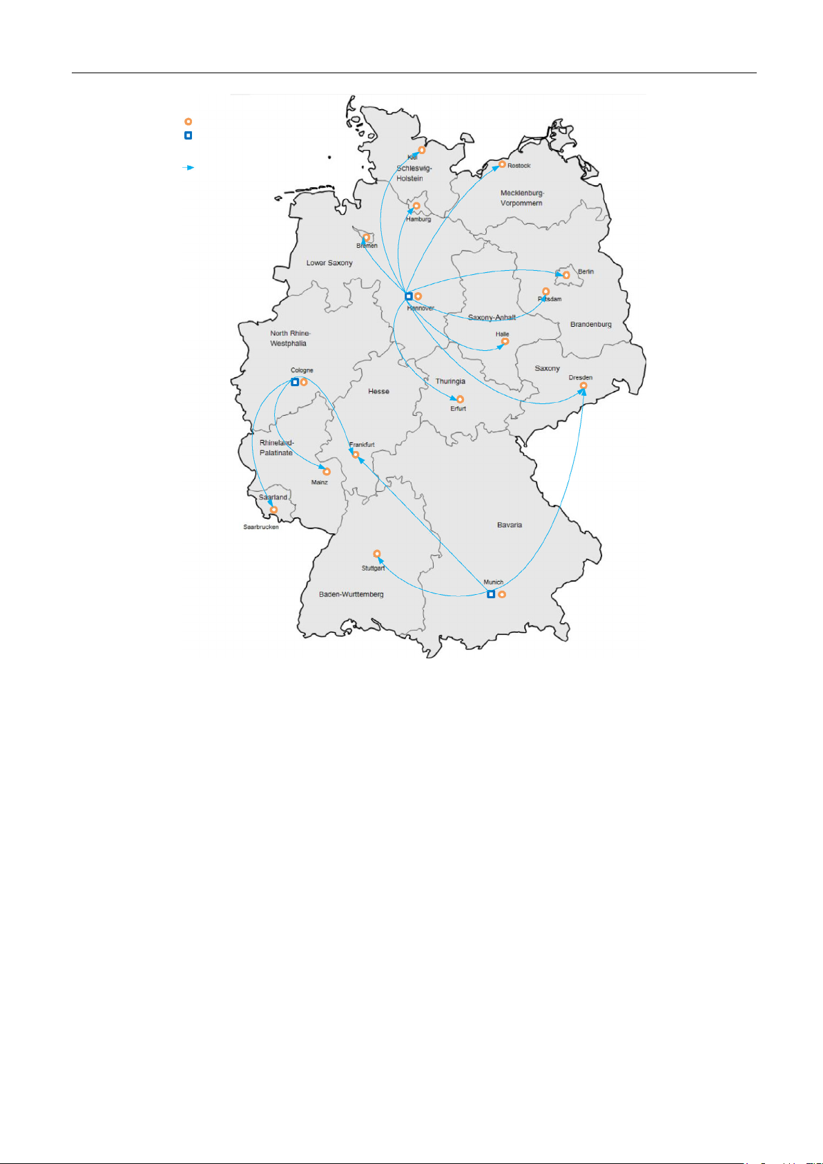
Chemical Engineering Research and Design 1 3 4 ( 2 0 1 8 ) 90–103 97 2030 Storage system Hydrogen production plant N Number of facility 1 Hydrogen flowrate 1 1 1 1 1 1 1 1 1 2 1 1 1 1 1 1 1 1
Fig. 5 – Hydrogen supply chain network for 2030 (Base scenario).
less than biomass or wind and solar energy (0.05 $ kg−1) (see
rent work is time-invariant: load/unload time, driver wage
Appendix A). Facilities and their interconnections are shown
expenses of transportation modes were not included, and it
in Fig. 5. The result is comparable with the outcomes of the
is close to the average unit cost expected in Europe in 2030
by work of Almansoori and Betancourt-Torcat (2016) for 2030.
(around 3.2 $ kg−1). In 2050, one extra facility is installed in
In both studies, coal gasification technology is selected as
Cologne. Additionally, plants are installed in Stuttgart, Berlin,
the most economic option. One of the production facility is
Frankfurt and Dresden (see Fig. 6).
installed in Hannover, another in Cologne, and the last one in
Munich for both studies. The production facilities locations 5.2.
“Green” scenario
promotes the product distribution to regional storage facil-
ities. Additionally, each production facility includes nearby
Despite the costs for water electrolysis technology, the “green”
storage facilities to satisfy the local hydrogen demand.
scenario considers the opportunity to satisfy the local hydro-
Furthermore, hydrogen is generated in liquid form.
gen demand and the household energy demand by wind- and
Germany has a well-developed railway infrastructure, i.e. the
solar energy (see Appendix C). It was founded that 3 or 8
railway tank car is selected as preferred transportation mode
large hydrogen facilities are required. The “green” scenario
in both studies. It is noted that a large part of the German
shows that hydrogen facilities need to be built in Potsdam
rail freight transport is electrified, which means that the rail
and Hannover by 2030, and in 2050 they need to be installed
transport is a clean type of distribution. As hydrogen is gener-
in Hannover, Potsdam, Munich, Mainz, Rostock, Halle, and
ated in liquid form, super-insulated spherical tanks are used
Kiel. The total costs of the HSC are approximately 27.9 and
to minimize heat loss. The total cost of HSC is approximately
73.5 Mio $ d−1 for 2030 and 2050 respectively, which means
7.8 and 19.3 Mio $ d−1 for 2030 and 2050 respectively, which
9.69 and 9.57 $ kg−1 of H2. The hydrogen price decreased by
means 2.63 and 2.51 $ kg−1 of H2 (the hydrogen price is 4.5%
4% from 2030 to 2050. However, it is not a reasonable price for
less in 2050 than in 2030). In case of hydrogen price decreas-
industry. In addition, expenses related with household energy
ing up to 2050, it might motivate to replace gasoline cars by
consumption account for 25.3 and 23.4 Mio $ d−1 for 2030 and
FCEVs in future. However, the hydrogen price (2.63 $ kg−1) is
2050 respectively, which shows electricity price reduction for
lower than from Almansoori’s work (3.03 $ kg−1) as the cur- this sector. 98
Chemical Engineering Research and Design 1 3 4 ( 2 0 1 8 ) 90–103 2050 Storage system Hydrogen production plant N Number of facility 1 Hydrogen flowrate 1 1 1 1 1 1 2 1 1 2 3 1 1 1 1 1 2 1 1 2 1 3
Fig. 6 – Hydrogen supply chain network for 2050 (Base scenario).
hydrogen production and the general power demand for any
Table 6 – HSC cost for two case studies in 2030.
electrical facility (excluding compression). Due to the high HSC costs (k$ d−1) Base case “Green” scenario
energy consumption an electricity price reduction can make Operating costs
water electrolysis technology feasible (see Appendix E).
Production and storage facilities 4795.0 18,442.5
The electricity price might be decreased by several Production feedstock fuel 471.0 6912.0
strategies such as integration of more renewable electricity Transportation 2.2 5.3
generation facilities such as wind mills, solar panels, wave Capital costs
pumps, or using off-peak electricity. However, the installa-
Production and storage facilities 2277.0 2512.0
tion of new energy facilities is only realistic in places with Transport 37.2 61.3
suitable geographical conditions (location with high avail- Total network cost 7582.4 27,933.1
ability of renewable energy sources) providing continuous
Hydrogen unit cost ($ kg−1) 2.6 9.7
energy generation. Moreover, the modification of existing con-
ventional methods or development of innovative methods is
necessary for reduction of conversion losses and capital costs 5.3. Case comparison
investment. There are a number of problems related with
conventional electrolysers such as safety risks due to leaks,
As shown in Table 6, the cost analysis has been done for
stack degradation, membrane deterioration, difficulties with
the two cases in 2030. For the hydrogen pathways, water
starting the system after shutdown, and freezing of mem-
electrolysis consumes more electricity than other technolo-
branes, especially during cold weather. All these problems
gies (see Appendix A). This energy consumption is about
require technological improvements. In addition, analysis of 50 kWh kg−1 H
2, with a specific power cost to supply the elec-
the impact of intermittency of renewable energy sources on
trolysers of 0.05 $ kWh−1. The capital- and operating costs
the electrolysis system performances and reliability, analysis
for a hydrogen production facility are only related to the
of possible cost parameters changing and demand shifting are
required power to achieve the targeted hydrogen production
required to map the uncertainty. Thus, there is a necessity
rate. The actual hydrogen production facility’s specific energy
of further R&D efforts on system design, power electronics
consumption is the sum of the specific power demand for
Chemical Engineering Research and Design 1 3 4 ( 2 0 1 8 ) 90–103 99
and process control to make hydrogen production by water
in terms of economy as well as implementation. Hydrogen electrolysis competitive.
transport in liquid form is preferable, distributed via rail-
way tank car and stored into super-insulated spherical tanks. 6. Conclusion
FCEVs penetration rate of 10% in 2030 and 30% in 2050 into pas-
senger transport shows a 4% reduction of the hydrogen price,
In this work, general optimization model for a HSC network
it can motivate to replace gasoline cars by FCEVs in future to
is proposed. The results shows that H2 has the potential diminish environmental impact.
to replace fossil fuel as a source of energy, especially for
Based on the obtained results, the building of HSC network
transportation. The model was applied to design strategies of
would be expensive at the current stage of technological devel-
developing the future HSC network in Germany, considering a
opment. However, the potential impact of renewable energy
full range of local factors and geographical conditions. More-
sources on the development of the cost effective and sustain-
over, the use of the water electrolysis technology is suitable
able HSC network takes place in future. Moreover, that can
option to satisfy the local hydrogen demand and the house-
be complemented by CO2 network, captured in industry, to
hold energy demand by existing installed wind- and solar
produce chemicals like methanol or heavy hydrocarbons can
power plants without environmental impact. Due to the high
further motivate a hydrogen based economy.
energy consumption an electricity price reduction can make
water electrolysis technology competitive. However, currently
Appendix A. Capital and unit production costs
coal gasification technology is still the dominant technology,
of hydrogen production technologies (Simbeck and Chang, 2002) Production technology Steam reforming Coal gasification Water electrolysis Biomass gasification Product form LH LH LH LH
Design production capacity t d−1 960.00 960.00 960.00 960.00 Plant availability d 329.00 329.00 329.00 329.00 Annual production 103 t 315.84 315.84 315.84 315.84
Fuel required per H2 generated unit kg−1 H2 3.16 5.33 47.60 11.26 Fuel consumed unit d−1 3033.60 5116.80 45,696.00 10,809.60 Fuel price $ unit−1 0.14 0.03 0.05 0.05 CO2 produced kg kg−1 H2 17.40 30.30 0.00 32.10
SMR/gasifier/electrolyzer $ unit−1 317.25 239.85 1110.67 506.70 CO2 cost $ kg−1 0.06 0.06 0.06 0.06 Energy cost $ kW−1 560.00
CO shift, cool and cleanup $ kg−1 d−1 CO2 20.00 15.00
Air separation unit $ kg−1 d−1 O2 28.00 27.00 O2 consumed per H2 generated 1.08 1.41 Dispenser rate kg h−1 4000.00 4000.00 4000.00 4000.00 Number of dispenser 10.00 10.00 10.00 10.00 H2 dispenser unit cost $ 100,000.00 100,000.00 100,000.00 100,000.00
Power consumption kWh kg−1 H2 11.00 11.00 58.60 11.00 Electricity cost $ kWh−1 0.05 0.05 0.05 0.05 Unit cost $ kg−1 d−1 H2 318.22 877.74 1110.67 1027.94 Size factor process 0.75 0.75 0.75 0.80
Unit liq/gas cost $ kg−1 d−1 H2 700.00 700.00 700.00 700.00 Size factor liq/gas 0.75 0.75 0.75 0.75 Unit storage cost $ kg−1 H2 19.00 19.00 19.00 19.00 Size factor of storage 0.70 0.70 0.70 0.70
Total process unit cost (UC) M$ 746.89 1149.74 1317.45 1307.23
General facilities cost 20% of UC M$ 149.38 229.95 263.49 261.44
Engineering Permitting 10% of UC M$ 74.69 114.97 131.74 130.72 Contingencies 10% of UC M$ 74.69 114.97 131.74 130.72
Working Capital, Land 5% of UC M$ 37.34 57.49 65.87 65.36
Total capital cost (CC) M$ 1082.99 1667.13 1910.30 1895.48 O&M 1% of CC M$ y−1 10.83 16.67 19.10 18.95 100
Chemical Engineering Research and Design 1 3 4 ( 2 0 1 8 ) 90–103 Fuel price M$ y−1 139.73 50.50 751.70 177.82 Electricity cost M$ y−1 173.71 173.71 925.41 173.71
Fixed operating cost 5% M$ y−1 54.15 83.36 95.51 94.78
Capital charges 12% of capital M$ y−1 129.96 200.06 22.92 227.46
Total Operating Cost M$ y−1 508.38 524.30 2020.96 692.71
Unit Production cost $ kg−1 1.61 1.66 6.40 2.19
Appendix B. Results of the hydrogen supply by grid point (Base scenario) Grid point, g Year 2030 Year 2050 H2 produced H2 imports by Local H2 produced H2 imports by Local by grid point grid point satisfaction of by grid point grid point satisfaction of (t d−1) (t d−1) H2 demand (t d−1) (t d−1) H2 demand (t d−1) (t d−1) 1 381.02 959.52 108.86 959.52 2 917.53 454.86 953.36 326.59 953.36 3 136.08 952.35 380.81 4 81.658 208.66 5 27.22 63.50 6 63.50 190.51 7 217.73 955.25 592.37 8 54.43 127.01 9 953.92 264.45 953.68 708.73 10 958.78 595.90 1908.75 1618.45 11 136.08 362.88 12 36.29 90.72 13 136.08 956.90 349.08 14 72.586 172.37 15 99.79 254.02 16 72.58 172.37 Total 2830.23 1515.02 1315.21 7639.81 2077.49 5562.32
Appendix C. Results of the hydrogen distribution by grid point (“Green” scenario) Grid point, g Year 2030 Year 2050 H2 produced H2 imports by Local H2 produced H2 imports by Local by grid point grid point satisfaction of by grid point grid point satisfaction of (t d−1) (t d−1) H2 demand (t d−1) (t d−1) H2 demand (t d−1) (t kg d−1) 1 381.02 1070.50 2 462.67 953.36 326.59 953.36 3 136.08 381.02 4 942.94 81.10 953.96 200.98 5 27.22 63.50 6 63.50 190.51 7 217.73 598.75 8 54.43 952.49 126.94
Chemical Engineering Research and Design 1 3 4 ( 2 0 1 8 ) 90–103 101 9 1897.41 264.45 1915.31 708.73 10 598.75 1623.89 11 136.08 958.41 359.66 12 36.29 90.72 13 136.08 353.81 14 72.58 958.51 169.25 15 99.79 952.42 253.87 16 72.58 172.37 Total 2840.35 2494.80 345.55 7644.45 4871.66 2772.79
Appendix D. Hydrogen flowrate for different scenario Base scenario “Green” scenario Year 2030 Year 2050 Year 2030 Year 2050 From To H2 From To H2 From To H2 From To H2 grid grid flowrate grid grid flowrate grid grid flowrate grid grid flowrate (t d−1) (t d−1) (t d−1) (t d−1) 2 1 381.02 1 1 959.52 4 2 462.67 2 2 953.36 2 7 27.22 2 2 953.36 4 3 136.08 4 2 18.14 2 13 54.43 3 3 380.81 4 8 54.43 4 3 381.02 9 3 136.08 3 4 208.66 4 13 136.08 4 13 353.81 9 4 81.65 3 8 127.01 4 14 72.58 8 1 254.02 9 5 27.22 3 15 235.87 9 1 381.02 8 7 571.54 9 6 63.50 7 1 108.86 9 5 27.22 9 7 27.22 9 8 54.43 7 2 63.50 9 6 63.50 9 10 1179.36 9 13 81.65 7 7 592.37 9 7 217.73 11 1 508.03 9 14 72.58 7 11 190.51 9 10 598.75 11 12 90.72 9 15 99.80 9 5 36.29 9 11 136.08 14 1 308.45 9 16 72.58 9 6 190.51 9 12 36.29 14 2 308.45 10 7 190.51 9 9 708.73 9 15 99.79 14 16 172.37 10 11 136.08 9 15 18.14 9 16 72.58 15 5 63.50 10 12 36.29 10 5 27.22 15 6 190.51 10 10 1618.45 15 10 444.53 10 11 172.37 10 12 90.72 13 2 263.09 13 13 349.08 13 14 172.37 13 16 172.37
Appendix E. HSC network cost depending of the energy price HSC costs “Green” scenario Electricity price reduction 10% 50% 100% Operating costs
Production and storage facilities (M$ d−1) 16.91 10.80 3.15 102
Chemical Engineering Research and Design 1 3 4 ( 2 0 1 8 ) 90–103
Production feedstock fuel (M$ d−1) 6.64 3.65 0.01 Transportation ($ d−1) 3475.30 2441.66 2213.80 Capital costs
Production and storage facilities (M$ d−1) 2.51 2.51 2.51 Transport ($ d−1) 51,498.89 41,912.51 37,230.80
Total network cost (M$ d−1) 26.12 17.01 5.71
Hydrogen unit cost ($ d−1) 9.38 6.10 2.05
Appendix F. Initial availability of energy sources Grid point, g Primary energy source, e Biomass (t d−1) Coal (t d−1) Natural gas (t d−1)
Renewable energy source (GWh d−1) Base scenario “Green” scenario 2030 2050 2030 2050 1 1.99 0.00 0.00 25.85 43.57 0.00 10.83 2 4.62 0.00 0.00 61.50 104.09 20.64 64.87 3 0.00 0.00 0.00 0.34 0.57 0.00 0.00 4 1.92 95,890.41 0.00 55.73 98.52 37.07 81.26 5 0.00 0.00 0.00 1.70 3.04 0.00 1.09 6 0.00 0.00 0.00 0.59 1.04 0.00 0.00 7 1.13 0.00 0.00 16.43 28.60 0.00 10.45 8 4.39 0.00 0.00 32.51 57.78 28.08 53.89 9 5.34 0.00 0.00 112.46 200.64 88.51 178.92 10 2.19 293,041.10 0.00 46.47 81.43 0.00 31.83 11 0.63 0.00 0.00 29.67 52.37 0.00 41.34 12 0.06 0.00 0.00 3.81 6.63 0.63 4.04 13 2.46 95,890.41 0.00 15.58 27.09 3.55 16.39 14 3.07 26,027.40 0.00 42.32 75.07 36.31 69.88 15 2.91 0.00 0.00 47.50 84.74 33.52 72.16 16 2.26 0.00 0.00 14.38 25.22 8.36 20.04 Total 32.97 510,849.32 0.00 506.85 890.41 256.67 656.99 References
Almansoori, A., Betancourt-Torcat, A., 2016. Design of
optimization model for a hydrogen supply chain under
Hake, J.F., Linssen, J., Walbeck, M., 2006. Prospects for hydrogen in
emission constraints — a case study of Germany. Energy 111,
the German energy system. Energy Policy 34, 1271–1283,
414–429, http://dx.doi.org/10.1016/j.energy.2016.05.123.
http://dx.doi.org/10.1016/j.enpol.2005.12.015.
Almansoori, A., Shah, N., 2012. Design and operation of a
Hugo, A., Rutter, P., Pistikopoulos, S., Amorelli, A., Zoia, G., 2005.
stochastic hydrogen supply chain network under demand
Hydrogen infrastructure strategic planning using
uncertainty. Int. J. Hydrogen Energy 37, 3965–3977,
multi-objective optimization. Int. J. Hydrogen Energy 30,
http://dx.doi.org/10.1016/j.ijhydene.2011.11.091.
1523–1534, http://dx.doi.org/10.1016/j.ijhydene.2005.04.017.
Amos, W.A., 1999. Costs of Storing and Transporting Hydrogen.
International Energy Agency (IEA), 2016. World Energy Outlook
Other Inf. PBD 27 Jan 1999; PBD 27 Jan 1999; PBD 27 Jan 1999. 2016.
Ball, M., Wietschel, M., Rentz, O., 2007. Integration of a hydrogen
http://www.iea.org/publications/freepublications/publication/
economy into the German energy system: an optimising
WEB WorldEnergyOutlook2015ExecutiveSummaryEnglishFinal.pdf.
modelling approach. Int. J. Hydrogen Energy 32, 1355–1368,
International Union of Railways, 2012. Railway Handbook 2012 —
http://dx.doi.org/10.1016/j.ijhydene.2006.10.016.
Energy Consumption and CO2 Emissions.
BM Verkehr Bau und Stadtentwicklung, 2013. The Mobility and
ISE, F.I. for S.E.S., n.d. Energy Charts [WWW Document].
Fuels Strategy of the German Government (MFS).
https://www.energy-charts.de/index.htm (accessed 5.25.17).
CO2.earth, n.d. 2100 Projections [WWW Document].
Pregger, T., Nitsch, J., Naegler, T., 2013. Long-term scenarios and
https://www.co2.earth (accessed 5.25.17).
strategies for the deployment of renewable energies in
Chemical Engineering Research and Design 1 3 4 ( 2 0 1 8 ) 90–103 103
Germany. Energy Policy 59, 350–360,
Simbeck, D.R., Chang, E., 2002. Hydrogen Supply: Cost Estimate
http://dx.doi.org/10.1016/j.enpol.2013.03.049.
for Hydrogen Pathways–Scoping Analysis. National
Schill, W.P., 2014. Residual load, renewable surplus generation
Renewable Energy Laboratory, doi:NREL/SR-540-32525.
and storage requirements in Germany. Energy Policy 73, 65–79,
Statistisches Bundesamt, n.d. Koordinierte
http://dx.doi.org/10.1016/j.enpol.2014.05.032.
Bevölkerungsvorausberechnung nach Bundesländern [WWW
Shafiee, S., Topal, E., 2009. When will fossil fuel reserves be
Document]. https://www.destatis.de/EN/Homepage.html.
diminished? Energy Policy 37, 181–189, (Accessed 25 May 2017).
http://dx.doi.org/10.1016/j.enpol.2008.08.016.
U.S. Energy Information Administration, 2017. Annual Energy
Siemens, L., n.d. Energiepark Mainz [WWW Document].
Outlook, doi:DOE/EIA-0383(2017).
http://www.energiepark-mainz.de/en/. (Accessed 20 March 2017).
Document Outline
- An outlook towards hydrogen supply chain networks in 2050 — Design of novel fuel infrastructures in Germany
- 1 Introduction
- 2 Network description and problem statement
- 2.1 Problem statement
- 2.2 Model description
- 2.2.1 Grid
- 2.2.2 Primary energy sources
- 2.2.3 Hydrogen production
- 2.2.4 Hydrogen physical form
- 2.2.5 Transportation mode
- 2.2.6 Storage facility
- 3 Model formulation
- 3.1 Household energy demand
- 3.2 Demand for a certain energy source
- 3.3 Hydrogen demand
- 3.4 Hydrogen generation
- 3.5 Hydrogen distribution
- 3.6 Hydrogen storage
- 3.7 Objective function
- 4 Case study
- 5 Results and discussion
- 5.1 Base case scenario
- 5.2 “Green” scenario
- 5.3 Case comparison
- 6 Conclusion
- Appendix A Capital and unit production costs of hydrogen production technologies (Simbeck and Chang, 2002)
- Appendix B Results of the hydrogen supply by grid point (Base scenario)
- Appendix C Results of the hydrogen distribution by grid point (“Green” scenario)
- Appendix D Hydrogen flowrate for different scenario
- Appendix E HSC network cost depending of the energy price
- Appendix F Initial availability of energy sources
- References
Tài liệu liên quan:
-

Ung dung game hoa trong cac chien dich MKT
18 9 -

Bao cao Chi so TMDT Viet Nam 2025
15 8 -

Thông tư quy định về việc phân quyền, phân cấp và phân định thẩm quyền quản lý nhà nước về giáo dục cho chính quyền địa phương
23 12 -

Nghị quyết về phát huy các giá trị di sản văn hóa gắn với phát triên du lịch bền vững tỉnh Khánh Hòa đến năm 2025, định hướng đến năm 2030
13 7 -

Quyết định phê duyệt Chiến lược phát triển du lịch Việt Nam đến năm 2030
13 7