Analysis of shield tunnel - International journal for numerical and analytical methods in geomechanics
Analysis of shield tunnel - International journal for numerical and analytical methods in geomechanics. Tài liệu được sưu tầm giúp bạn tham khảo, ôn tập và đạt kết quả cao. Mời bạn đọc đón xem.
Môn: Tài liệu Tổng hợp 3.6 K tài liệu
Trường: Tài liệu khác 3.9 K tài liệu
Tác giả:


Preview text:
INTERNATIONAL JOURNAL FOR NUMERICAL AND ANALYTICAL METHODS IN GEOMECHANICS
Int. J. Numer. Anal. Meth. Geomech., 2004; 28:57–91 (DOI: 10.1002/nag.327) Analysis of shield tunnel
W. Q. Ding1, Z. Q. Yue2,n,y, L. G. Tham2, H. H. Zhu1, C. F. Lee2 and T. Hashimoto3
1 Department of Geotechnical Engineering, Tongji University, Shanghai, China
2 Department of Civil Engineering, The University of Hong Kong, Pokfulam Road, Hong Kong, China
3 Geo-Research Institute, Osaka, Japan SUMMARY
This paper proposes a two-dimensional finite element model for the analysis of shield tunnels by taking
into account the construction process which is divided into four stages. The soil is assumed to behave as an
elasto-plastic medium whereas the shield is simulated by beam–joint discontinuous model in which curved
beam elements and joint elements are used to model the segments and joints, respectively. As grout is
usually injected to fill the gap between the lining and the soil, the property parameters of the grout are
chosen in such a way that they can reflect the state of the grout at each stage. Furthermore, the contact
condition between the soil and lining will change with the construction stage, and therefore, different stress-
releasing coefficients are used to account for the changes. To assess the accuracy that can be attained by the
method in solving practical problems, the shield tunnelling in the No. 7 Subway Line Project in Osaka,
Japan, is used as a case history for our study. The numerical results are compared with those measured in
the field. The results presented in the paper show that the proposed numerical procedure can be used to
effectively estimate the deformation, stresses and moments experienced by the surrounding soils and the
concrete lining segments. The analysis and method presented in this paper can be considered to be useful
for other subway construction projects involving shield tunnelling in soft soils. Copyright # 2004 John Wiley & Sons, Ltd. KEY WORDS:
subway construction; shield tunnelling; soil–structure interaction; numerical procedure;
finite element method; ground settlement; lining; soft soils 1. INTRODUCTION
Since 1950s, urban developments in many cities have experienced continuous growth and
expansion. Because of the large populations and shortage of land resources, these cities have
always had a strong demand for efficient, economic and environmental friendly urban civil
infrastructure systems to accommodate the daily and routine travels of thousands and millions
of commuters. The subway system is an obvious solution to meet the demand. To minimize the
nCorrespondence to: Dr. Q. Z. Q. Yue, Department of Civil Engineering, The University of Hong Kong, Pokfulam Road, Hong Kong, China. y E-mail: yueqzq@hkucc.hku.hk
Contract/grant sponsor: Research Grant Council of Hong Kong SAR Government
Contract/grant sponsor: Hong Kong Jockey Club Charities Trust Received 23 August 2002 Revised 9 July 2003
Copyright # 2004 John Wiley & Sons, Ltd. Accepted 30 August 2003 58 W. Q. DING ET AL.
impact on the existing traffic during construction, tunnelling is usually adopted for the
construction of the subway. Because of its efficiency and safety, shield tunnelling is one of the
most popular tunnelling methods for the construction of subway tunnels in soft soil ground.
Over the last 30 years, the shield tunnelling method has experienced continuous improvement
and development. New shield tunnelling methods including the earth pressure balanced shield,
the slurry shield, the simultaneous backfill grouting as well as some improved grouting materials
have been introduced and developed in recent years [1].
Shield tunnelling will inevitably induce ground deformation and the surrounding soils will
also act on the shield lining segments. Quantitative and accurate prediction of such soil and
structure interaction will be of significant importance in many aspects including lining segment
design, construction safety, ground settlements, potential damage to existing structures and
facilities, and operation of the subway system.
Peck [2] developed an empirical method for the ground settlement associated with tunnelling
in soft soils by assuming the settlement trough to be a Gaussian distribution curve. The
actual ground settlement is predicted based on the estimation of the ground loss ratio. This
method was used and improved by many engineers and researchers such as Clough and
Schmidt [3] and Rowe et al. [4]. Recently, Schmidt [5] has proposed the semi-empirical
error function method for the estimation and prediction of ground settlement. Though these
empirical or semi-empirical methods are useful in the evaluation of the ground settlements
caused by shield tunnelling construction, they must be applied with caution as they may not be
applicable to situations significantly different from the cases on which they are based on Wang [6].
Another important design parameter is the load acting on the lining. Such load can be
taken to be either the sum of the overburden pressure and water pressure or that determined
using Terzaghi’s formula, Schulze–Duddeck method or other empirical methods. It is noted
that such load only considers the final state that is after the completion of the shield tunnelling.
To provide a better simulation of the interaction between the lining and soil, beam–
spring models, in which the lining and soil are modelled by beam and spring, respectively,
can be adopted. As shield tunnel lining is composed of several concrete segments, a number of
researchers and engineers had also taken into consideration the effects of the segment ring
joints [7, 8] in their studies. Lee and Ge [9] suggested an equivalent method to determine
the correction factor for approximating a jointed shield-driven tunnel lining as a continuous
ring structure under a plane strain condition. The present literature review has revealed that
there are three widely accepted methods for modelling the effects of shield segment joints [10, 11].
Furthermore, shield tunnelling usually adopts staged construction and supporting techniques.
Consequently, the responses such as soil displacements and lining forces induced by the
construction will be different at different stages. It is believed that an optimal construction
process can improve the safety and reduce the disturbance to the surrounding soils. Hence, it
becomes very important to take into account the actual construction process in the shield
tunnelling design [12, 13]. Due to the complex nature of the problems, one may have to resort to
numerical approach for analysing the problems. It is well known that the finite element method
is a powerful tool for the analysis of soil–structure interaction in geomechanics and it has been
applied to tunnel excavations by taking into account the construction process, the different soil
layers, complex geometries, various loading conditions and soil–lining interfaces [14]. Though
shield tunnelling, strictly speaking, is a three-dimensional and time-dependent soil–structure
Copyright # 2004 John Wiley & Sons, Ltd.
Int. J. Numer. Anal. Meth. Geomech. 2004; 28:57–91 ANALYSIS OF SHIELD TUNNEL 59
interaction problem [15–18], many engineers and researchers have demonstrated that the two-
dimensional finite element models can still give a fairly accurate prediction on the behaviour of
the tunnel [12, 19, 20]. Benmebarek et al. [21] proposed two methods for taking into account the
three-dimensional effects in a two-dimensional model. Further assessment of two-dimensional
models in analysing shield tunnelling was reported in a recent publication by Negro and de Queiroz [22].
In this paper, we propose a two-dimensional finite element method for analysing shield
tunnels during construction. The construction of each lining segment of a shield tunnel is
divided into four stages. To model the discontinuous displacements between segments, a beam–
joint discontinuous model is adopted for simulating the shield action. Moreover, the changes
from fluid and solid states of the backfill grout at different stages are also considered.
Furthermore, stress-releasing coefficients are used to account for the different contact conditions
between the soil and external lining surface. These coefficients are estimated based on field
measured settlements and professional experiences. The numerical results obtained by the
present model are compared with those measured during the construction of the No. 7 Subway
Line Project in Osaka, Japan. The comparison shows that the proposed model can be used to
estimate the deformation, stresses and moments experienced by the surrounding soils and the
concrete lining segments during tunnelling. 2. BACKGROUND
During shield tunnelling, the shield will advance segment by segment with a balanced soil
pressure that supports the soil. After cutting through a length of a segment, the lining will
then be installed. The lining is essentially an assembly of concrete segments linked by bolts
which joints will be covered with waterproof flexible plates. Before the shield tail is
detached, grout will be injected into the gap between the surrounding soil and the lining.
After grouting, the shield will move forward. As the grout hardens and consolidates, the
surrounding soil will deform and induce pressures on the lining. Consequently, the ground will
settle gradually as well. All movements will cease only when a state of equilibrium state is reached.
Field observations have confirmed that the ground movements and the earth pressure on the
lining segments have developed according to the construction process of the shield tunnelling
[1, 21, 23–25]. Factors affecting ground movements due to shield tunnelling have been
summarized in recent publications by Nomoto et al. [25] and Hashimoto et al. [1, 26]. The
construction process is one of the most important factors. Closer study of the field observations
has revealed that the construction process for a segment can be divided into four stages below:
Stage 1}Balanced cutting and shield supporting. This stage includes face cutting and
shield advancing. The existing soil pressure in the cutting face is balanced by pressure
from the machine behind the cutter. Consequently, the stress changes due to the cutting and
the balancing pressure will not result in significant soil movement. Furthermore, the
surrounding soil outside the shield will not be able to release its stress due to the rigid
support of the shield. However, one has to consider the possible disturbance on the surrounding
soil due to over-cutting, snaking and friction between the shield and the soil when the shield advances.
Copyright # 2004 John Wiley & Sons, Ltd.
Int. J. Numer. Anal. Meth. Geomech. 2004; 28:57–91 60 W. Q. DING ET AL.
Stage 2}Backfill grouting. The second stage is to install the lining segments and to backfill the
gap at the shield tail with grout. The lining will form a circular ring within the shield tail cover
plate. Once the shield moves forward, a gap between the soil and the lining segment will be
created. A grout must be simultaneously injected to backfill the gap space. The amount of grout
is usually equal to 1.2–1.3 times of the gap volume and the grout pressure is between 0.2 and
0:4 MPa: Such backfill grouting has three functions: *
preventing soil deformation immediately after the shield tail is detached, *
stabilizing lining segments, and *
improving tunnel water-proof performance.
The soil will start to interact with the lining although the grout is still in a fluid state. It is
noted that this backfill grouting serves a controlling measure to prevent soil deformation.
Excessive grout volume and pressure may lead to soil heave around the shield tail and must be avoided.
Stage 3}Grout hardening. This stage is a transient stage. The grout will harden and consolidate,
and the soil deformation will also increase with time though its rate decreases. The lining
segments and ground soil interaction will increase with time until an equilibrium state is
reached. It is, therefore, necessary to assess the effects of the grout hardening and pressure
distribution on the response of the lining structure at this stage.
Stage 4}Hardened grout. In the final stage, the grout becomes hardened and gains its full
stiffness and strength. The settlement will almost cease to increase.
3. NUMERICAL PROCEDURES FOR SHIELD TUNNELLING
In this paper, a two-dimensional finite element model is developed for modelling shield
tunnelling process. As such process is a very complicated one, exact simulation is almost
impossible. Therefore, the model only tries to take into account major factors, namely the
complex properties of the soil materials, the snaking of the shield direction, the volume loss, the
grout properties and pressure, the joints of lining segment, and the construction process.
Following the standard finite element procedures, one has to obtain the initial stress before the
construction simulation can be carried out. The initial stresses at any point i is calculated by the following equations: P sy0 ¼ gjHj ð1Þ
sx0 ¼ K0ðsy0 PwÞ þ Pw
where sy0 and sx0 are the vertical and horizontal initial earth stresses, respectively, g is the unit j
weight of the jth earth stratum above the point; Hj is the corresponding thickness; K0 is the
lateral earth pressure coefficient, and Pw is the water pressure at the point.
As pointed out in Section 2, the construction of a tunnel segment can be divided into
four stages. As the soils behave non-linearly during the construction, an elasto-plastic
model is adopted to model the soil. Similarly, the lining segment and the joints between
lining segment are modelled by adopting appropriate curved members. Different models
are adopted to simulate the grout as its behaviour is very much different at the various
Copyright # 2004 John Wiley & Sons, Ltd.
Int. J. Numer. Anal. Meth. Geomech. 2004; 28:57–91 ANALYSIS OF SHIELD TUNNEL 61 stages. To take into account such non-linear complex problems, an incremental-
iterated technique with constant stiffness within each construction stage is used in the
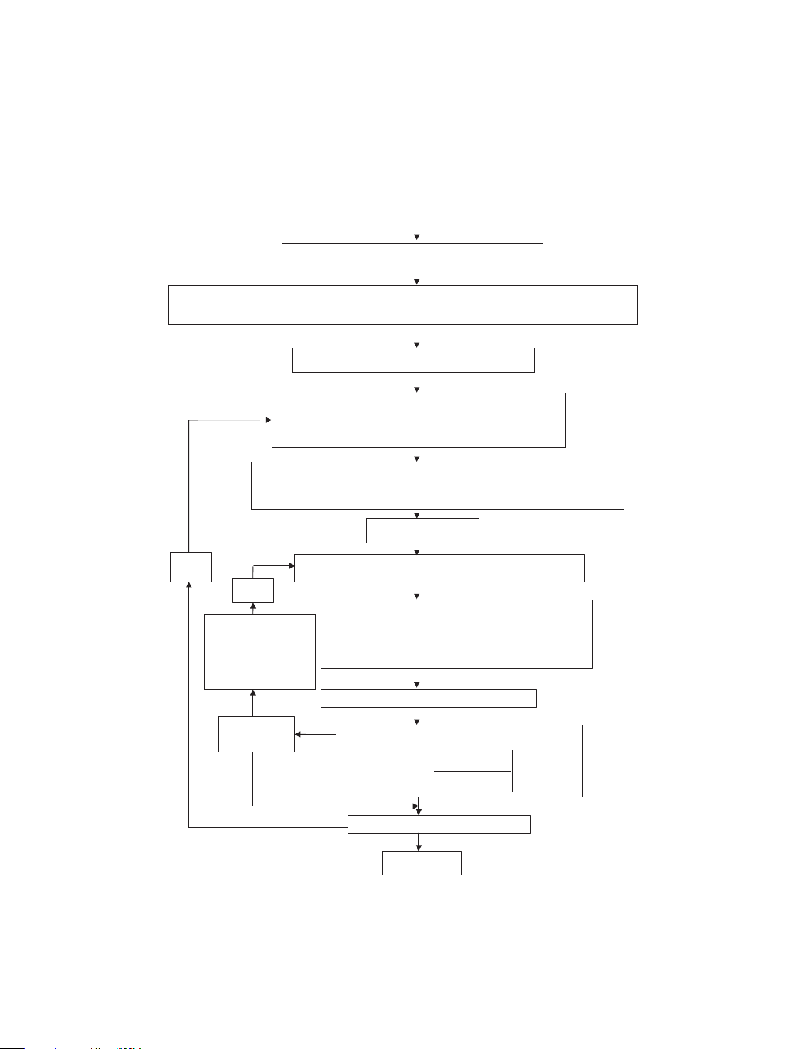
analyses. A flow chart illustrating the above FEM simulation for the soil–structure interaction
analysis of shield tunnelling is presented in Figure 1. Mathematically, the solution process
Input calculating data and controlling information
Calculate initial or current earth stress and stress releasing equivalent nodal forces { F ∆ }rea
Construction stage (stress releasing step): j=1
Calculate newly added and stress releasing nodal forces at j j
current construction stage: α { F ∆ } , F ∆ rea { }add j ζ
Form element and global stiffness matrix: [K ] K ini + ∑ [∆ ] ζ =1 Iteration step: k=1 j=j+1 jk Solve FEM equation, gain: { δ ∆ } k=k+1 jk jk
Calculate incremental strain and stress: { ε ∆ },{ σ ∆ }, Nonlinear equivalent nodal forces:
then gain total displacement, strain and stress. { jk F ∆ }non
Soil and contact element nonlinear analysis No No Iteration step:
New over-excessive stress element exists? k ≥ N Yes ∆ e σ σ jk − ∆ p jk Precision satisfied ? < . 0 00001 p σ σ j (k − − ∆ 1) jk Yes No Construction stage: j ≥ 4 Yes Output results
Figure 1. Flow chart of the finite element simulation for shield tunnelling.
Copyright # 2004 John Wiley & Sons, Ltd.
Int. J. Numer. Anal. Meth. Geomech. 2004; 28:57–91 62 W. Q. DING ET AL. can be expressed as ! X j ½K þ ½ f þ f þ f ð ini DKz
Dd jkg ¼ a jfDF grea DF jgadd DF jkgnon 2Þ B¼1
where j ¼ 1–4 and k ¼ 1–N ; N is the number of non-linear iterative steps; ½Kini is the initial
stiffness matrix of soil ground and structure (if it exists) before excavation; ½DKz is the
increment or decrement stiffness matrix of the soil ground excavated and the supporting
structure installed or removed at the construction stage z; fDF grea is the vector of the stress
releasing equivalent nodal forces due to the stress state of the previous construction process
acting along the currently excavated boundary. For one construction (excavation) process, it is
due to the initial stress state; fDF jgadd is the vector of newly added nodal load at construction
stage j; fDF jkgnon is the vector of current incremental equivalent excessive nodal forces caused P R
by non-linear stress. fDF jkg ¼ f non
BgTfDsag dV where fBg is strain matrix and fDsag is e Ve
the incremental non-linear stress vector; fDd jkg is the vector of incremental nodal displacement
at the stage j and iterative step k; a j is the stress releasing coefficient at construction stage j:
The iteration for each stage will cease after 10 iterative steps, that is N ¼ 10; or the prescribed
iterative precision is achieved. In the analysis, the iterative precision is chosen to be Dse Dsp jk jk 50:00001 ð3aÞ sjðk1Þ Dsp jk
where Dse and Dsp are the elements of the vectors of incremental elastic stress matrix fDse g jk jk jk
and plastic stress matrix fDsp g at the stage j and the iterative step k; respectively, and s jk jðk1Þ is
the corresponding total stress at the stage j and the iterative step k 1: Dse and Dsp can be jk jk
estimated using the following equations:
fDse g ¼ ½D½BfDd jkg ð3bÞ jk fDsp g ¼ ½D jk p½BfDd jk g ð3cÞ
where ½D and ½Dp are the elastic and plastic material property matrices, respectively.
After solving Equation (2), one can obtain the total displacement fdig; strain feig and stress
fsig at the construction stage i ði ¼ 1; 2; 3; 4Þ using the following equations: X i X N fdig ¼ fd0g þ fDd jkg j¼1 k¼1 X i X N feig ¼ fe0g þ fDe jkg j¼1 k¼1 X i X N fsig ¼ fs0g þ fDs jkg ð4Þ j¼1 k¼1
where fd0g and fe0g are the initial displacement and strain respectively, they are usually set to
zero. fs0g is the initial earth stress; fDe jkg and fDs jkg are the vectors of the incremental strain
and stress releasing step (construction stage) j and the iterative step k; respectively.
Furthermore, the lining internal forces (hoop force, shear force and bending moment) can
then be determined from the displacements.
Copyright # 2004 John Wiley & Sons, Ltd.
Int. J. Numer. Anal. Meth. Geomech. 2004; 28:57–91 ANALYSIS OF SHIELD TUNNEL 63
4. A CASE STUDY: SHIELD TUNNELLING FOR OSAKA NO. 7 SUBWAY LINE
Extensive monitoring was carried out during the construction of a tunnel of the Osaka Subway
Line. The results are readily available. This case history is used to assess the accuracy that can be
achieved by the present approach. For completeness, a brief of the relevant information will be
given and more detailed information can be found in the report prepared by the Japanese
Research Society of Construction Maintenance Techniques [27]. 4.1. General
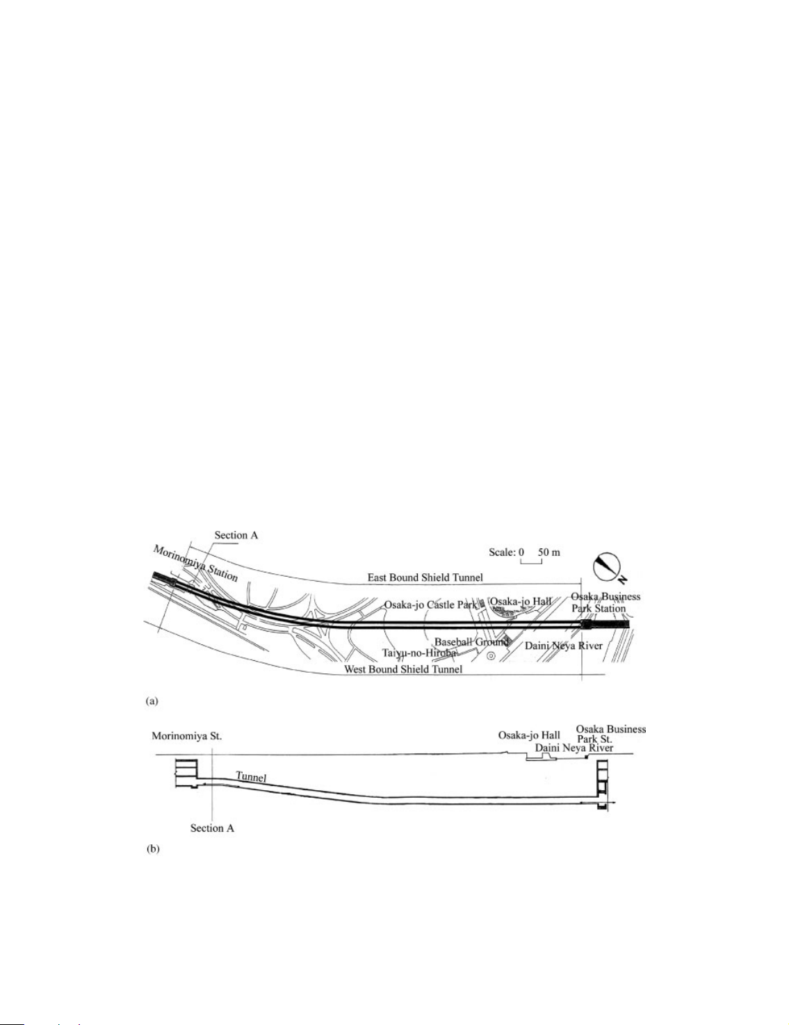
Figure 2 shows the general arrangement and longitudinal profile of the No. 7 Subway Line
Project in Osaka, Japan. The subway is between the Morinomiya Station and the Osaka
Business Park Station. Its east bound tunnel line is about 970:4 m long. Its west bound tunnel
line is about 974:5 m long. The tunnels are about 16–30 m below the soil ground surface. The
lining is of reinforced concrete and each segment is 1:2 m wide and 280 mm thick, and has the
outer diameter 5:3 m: Two 5:44 m in diameter earth pressure balanced shield machines with
synchronous grouting technique were used to construct the tunnels. In this paper, we will focus
on Section A of the west bound tunnel. 4.2. Ground conditions
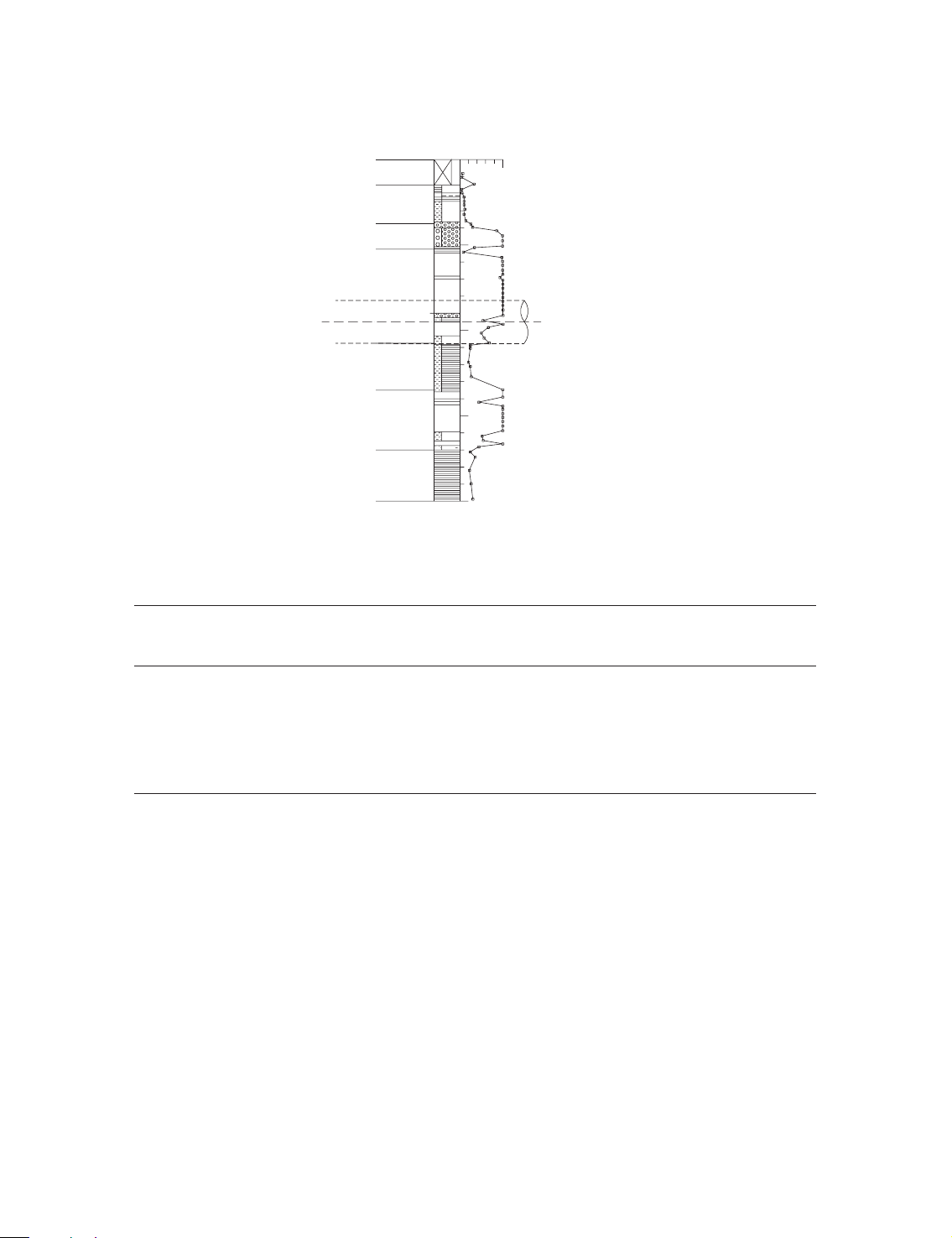
Figure 3 shows the soil stratum characteristics at Section A of the tunnels. There are three
different clayey and sandy soil strata, i.e. AC1, AC2 and AS1, above the proposed tunnel. The
tunnel is located at about 20 m below the ground. The tunnel passes through a sand layer, AS2,
Figure 2. General layout of the Osaka No. 7 Subway Line: (a) line plan; and (b) tunnel profile.
Copyright # 2004 John Wiley & Sons, Ltd.
Int. J. Numer. Anal. Meth. Geomech. 2004; 28:57–91 64 W. Q. DING ET AL. 0 50 Standard Penetration Test (SPT) value Soil layer: Ac1 Ac2 As1 -10 As2 Tunnel -20 Ac3 As3 -30 Ac4 -40 Depth (m)
Figure 3. The soil layer of Section A.
Table I. The adopted ground soil parameters. Soil Thickness Average Elastic Internal Unit Lateral layer of per layer value of modulus Poisson’s friction Cohesion weight pressure name Hj ðmÞ SPT N E ðkPaÞ ratio m angle j ð8Þ C ðkPaÞ g ðkN=m3Þ coefficient j K0 AC1 2.0 2.50 8500 0.43 0.0 25.0 16.0 0.75 AC2 5.5 6.11 20774 0.43 0.0 61.1 16.7 0.75 AS1 3.0 34.00 39500 0.35 37.6 0.0 16.6 0.55 AS2 11.0 43.05 49003 0.35 40.4 0.0 16.5 0.55 AC3 5.0 11.80 40120 0.43 0.0 118.0 17.0 0.75 AS3 7.0 42.64 48572 0.35 40.3 0.0 16.5 0.55 AC4 26.0 13.80 46920 0.43 10.0 138.0 17.4 0.75
and a clayey layer, AC3. The thicknesses of these layers are about 11 and 5 m; respectively.
Below the AC3 stratum, there are a sandy stratum, AS4, and a clayey stratum, AC4. The
permanent ground water level is at about 3 m below the ground surface. The standard
penetration test results revealed that the three upper clayey soil strata (AC1–AC3) had a SPT N -
values from 2.5 to 11.8 whereas the three sandy soil strata (AS1–AS3) had SPT N -values ranging
from 34 to 43.05 (Figure 3 and Table I).
4.3. Instrumentation system for monitoring
In order to verify the shield tunnelling design and the settlement prediction, an instrumentation
system was installed before and during the tunnel construction to monitor the ground settlement
Copyright # 2004 John Wiley & Sons, Ltd.
Int. J. Numer. Anal. Meth. Geomech. 2004; 28:57–91 ANALYSIS OF SHIELD TUNNEL 65 z depth (m) y 0 S1 -0.25 S1 ~ S5 Measuring points S2 -10.8 S3 -14.8 S4 -15.8 S5 -16.3 180° 270° o' 90° θ 0° East Bound West Bound to be constructed being constructed and examed in this paper Section A-A
Figure 4. The locations of the settlement gauges.
and lining structural performance. Figure 4 shows the arrangement of the five settlement
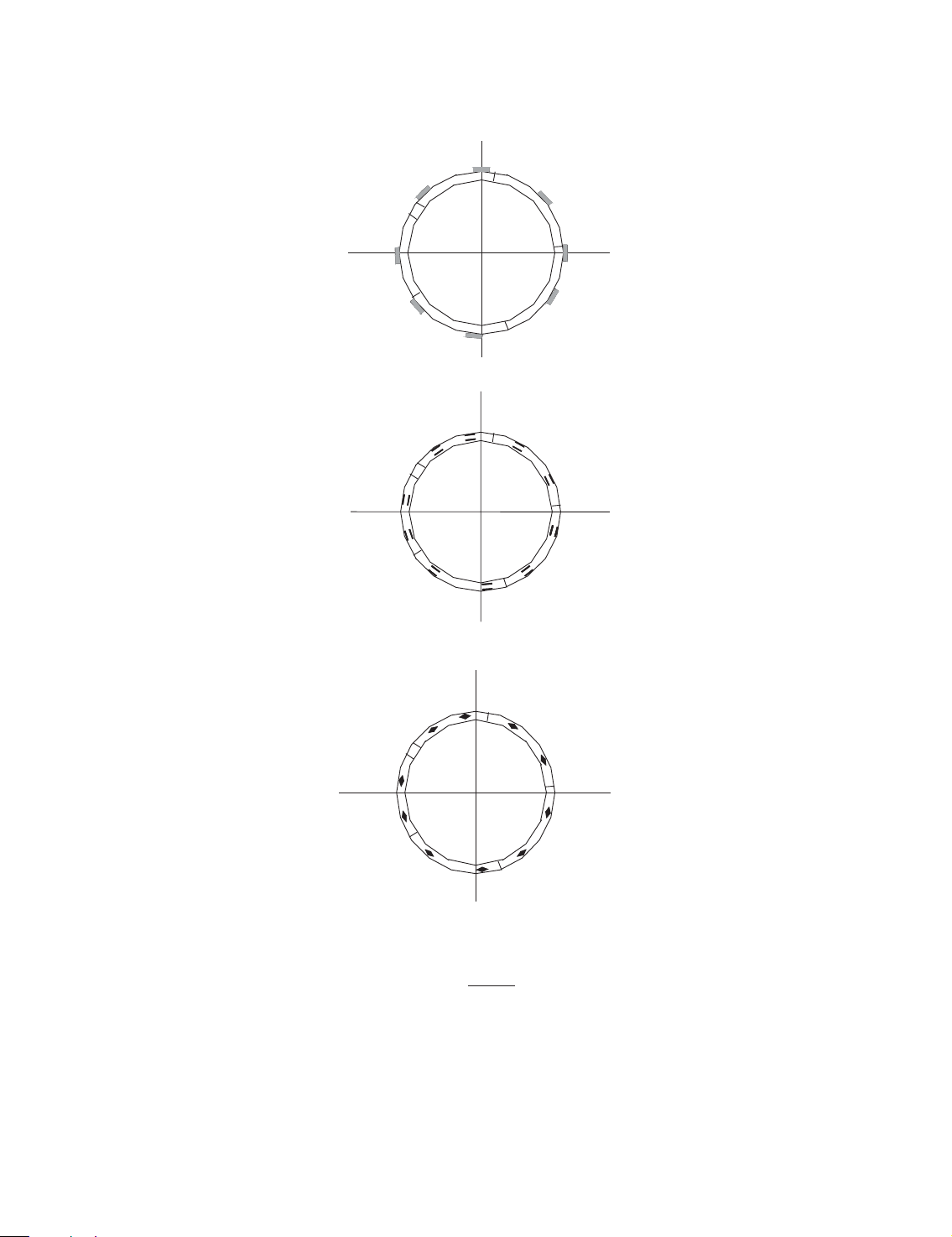
monitoring points in the soil right above the west bound tunnel. Figure 5(a) shows the
arrangement of eight earth pressure cells installed to measure the soil pressure acting on the
outer surface of the concrete lining segments. Gauges are installed to measure moment as well as
hoop forces. Their locations are shown in Figure 5(b) and 5(c), respectively.
4.4. Constitutive model for the surrounding soil
An elasto-plastic constitutive model was used in this paper for the soils surrounding the tunnel.
The model employs the classical Drucker–Prager yield criterion and the Reyes elasto-plastic
matrix [28] after a careful examination of the soil properties [12]. The following empirical
equations are used to determine the Young’s modulus E ðkN=m2Þ the internal friction angle j,
the lateral pressure coefficient K0 and Poisson’s ratio m for the sandy soil:
E ¼ 3800 þ 1050N ð5aÞ pffiffiffiffiffiffiffiffiffi j ¼ 15 þ 15N ð5bÞ K0 ¼ 1 sin j0 ð5cÞ
Copyright # 2004 John Wiley & Sons, Ltd.
Int. J. Numer. Anal. Meth. Geomech. 2004; 28:57–91 66 W. Q. DING ET AL. EP3(180°) 180° EP4(224°) EP2(131°) 270° 90° EP5(272 EP1(90 °) °) EP8(58°) EP6(310°) EP7(355°) 0° (a) M04(188°) 180° M05(214 M03(151 °) °) M02(116°) M06(261°) 270° 90° M07(288°) M01(75°) M08(323°) M10(37°) 0 M09(5 ° °) (b) AF04(188˚) 180˚ AF05(214˚) AF03(151˚) AF02(116˚) AF06(261˚) 270˚ 90˚ AF07(288˚) AF01(75˚) AF08(323˚) AF10(37˚) 0° AF09(5˚) (c)
Figure 5. The locations of: (a) earth pressure cells; (b) moment gauges; and (c) hoop force gauges. K m ¼ 0 ð5dÞ 1 þ K0
where j is the internal friction angle, j0 is effective internal friction angle, K0 is the lateral
pressure coefficient, N is the number of standard penetration test (SPT) value.
Copyright # 2004 John Wiley & Sons, Ltd.
Int. J. Numer. Anal. Meth. Geomech. 2004; 28:57–91 ANALYSIS OF SHIELD TUNNEL 67
For the clayey soils, we used the following empirical relations: E ¼ 170qu ð6aÞ K0 ¼ OCR0:3 0:5 ð6bÞ qu c ¼ ð6cÞ 2 N qu ¼ ð6dÞ 50 K m ¼ 0 ð6eÞ 1 þ K0
where c is the cohesion ðkN=m2Þ; qu is the unconfined compression strength (MPa), and OCR is the over-consolidation ratio.
The parameters of the seven soil strata are given in Table I.
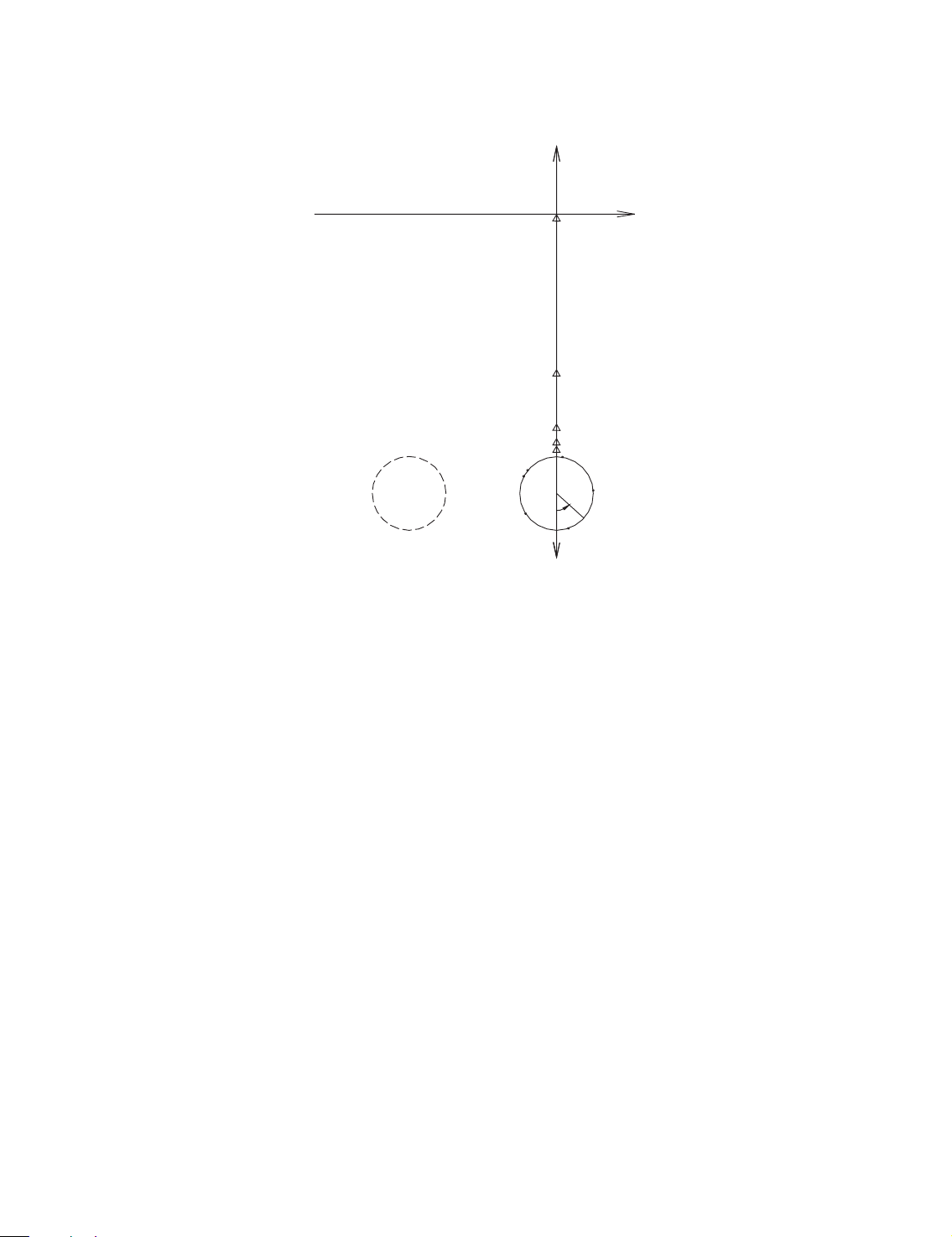
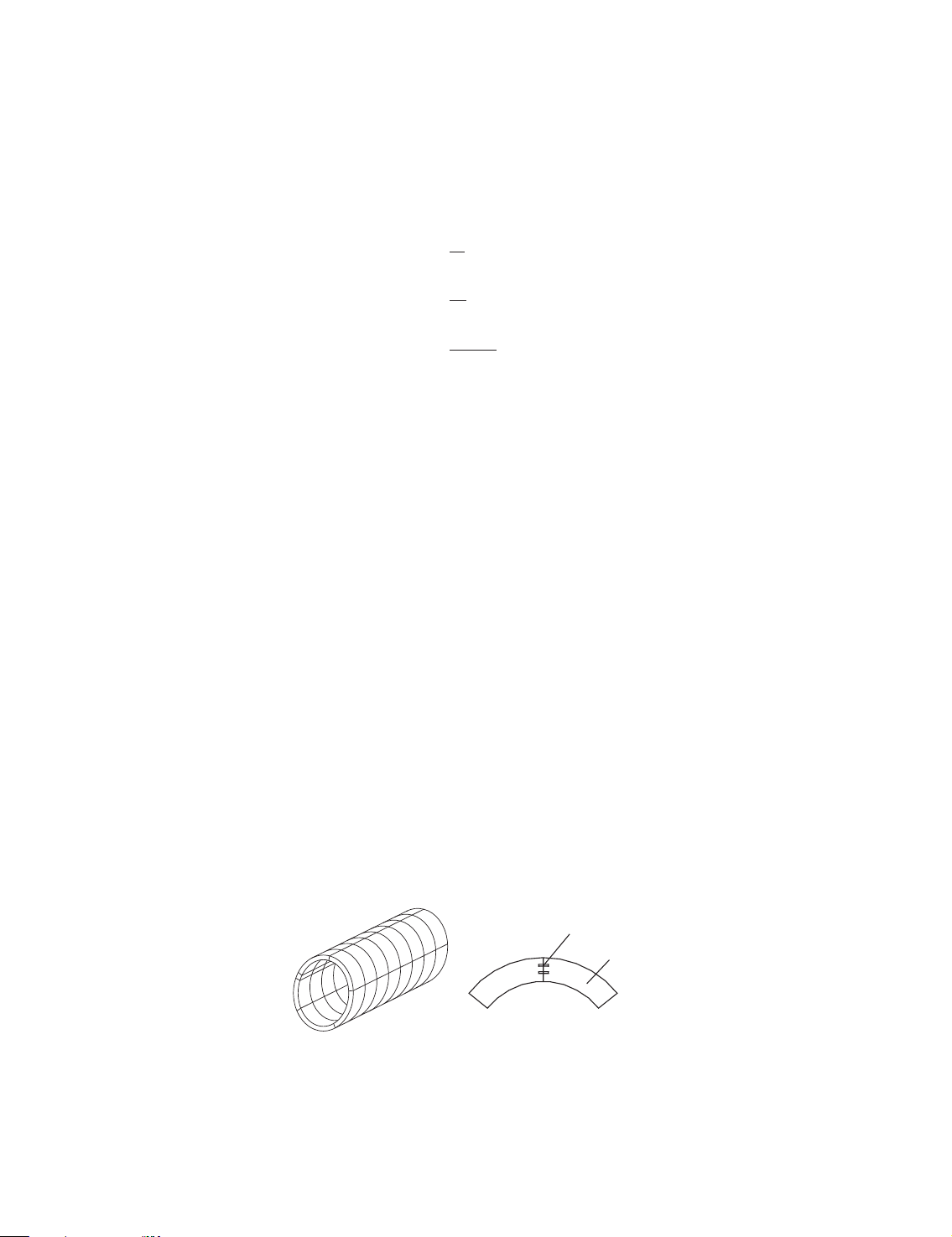
4.5. Modelling of the shield lining
Figure 6 shows a typical reinforced concrete segment with a circular-arc-shape. For such
segment, one can adopt curved beam elements to simulate its action (Figure 7). As flexible plates
were used to ensure flexible joint contact between the concrete segments, the joints will
smoothen the stress concentration but they have some inherent discontinuous characteristics in
transfering deformation. In this study, we have proposed a special joint element to represent the
flexible contact between any two adjacent segments. A detailed description of the model is given in Appendix A.
Based on the test results, the following lining parameters are adopted: the Young’s modulus
E ¼ 3:5 107 kN=m2; the rectangular cross-section area A ¼ 0:28 m2; the bending moment of
inertia I ¼ 1:83 103 m4; the joint parameters: kW ¼ 2:5 108 kN m=rad=m2; kn ¼ 6:55
107 kN=m3; ks ¼ 2:5 107 kN=m3: 4.6. Modelling of the grout
In the analysis, both the grout stiffness and grout pressure have to be modelled adequately and
the details of the models are outlined as follows:
(a) Grout stiffness. In this study, we adopted the Goodman joint model to represent such grout
contact property [28]. In this model, the element thickness is assumed to be zero and the
stiffnesses are defined in terms of the normal and tangential stiffness. The normal stiffness Kn joint segment
Figure 6. Shield tunnel lining segment.
Copyright # 2004 John Wiley & Sons, Ltd.
Int. J. Numer. Anal. Meth. Geomech. 2004; 28:57–91 68 W. Q. DING ET AL. Joint n Beam 2 1 s
Figure 7. Beam–joint discontinuous model.
depends on the grout deformation modulus whereas the tangential stiffness Ks is related to the
sliding feature of the contact.
If the normal contact stress sn is compressive, i.e. it has positive value, one can assume that
the yield criterion of the contact element will follow the Mohr–Coulomb function, that is
f ¼ jtsj ðcj þ sntgj Þ ð7Þ j
where cj and j are, respectively, the cohesion and internal friction angle of the contact element, j
ts is the total shear stress on the contact element.
One can show readily that the elastic property matrix ½D and plastic property matrix ½Dp for
the ideal plastic and plane strain situation can be expressed as " # Ks 0 ½D ¼ ð8aÞ 0 Kn " # 1 K2 K s sS1 ½Dp ¼ ð8bÞ S0 KsS1 S21
where S0 ¼ Ks þ Kntg2j ; S : j
1 ¼ Kntgjj
The grout initially is in fluid state and it hardens gradually. Therefore, different parameters
should be used to simulate the behaviour of the grout. A brief description is given below to
explain how to adopt different grout parameters at the different construction stages.
In Stage 2, the grout is in the fluid state, and therefore, the tangential contact stiffness Ks is
close to zero. Although the liquid is incompressible, the trapped air voids can be compressed.
Assuming 15% of the total grout volume is occupied by air voids, the relation between the
grouting pressure and volumetric strain can be expressed as P e a v ¼ 0:15 1 ð9Þ Pa þ Pg
where Pa and Pg are the atmospheric pressure and the grouting pressure, respectively. In the
numerical calculations, we assumed Pa ¼ 0:1 MPa and Pg ¼ 0:15 MPa: The value of the normal
contact stiffness Kn can be estimated using the equation below Pg Kn ¼ ð10Þ ev t0
where t0 is the thickness of shield tail void and it equals to 0:07 m for the present shield tunnel.
Copyright # 2004 John Wiley & Sons, Ltd.
Int. J. Numer. Anal. Meth. Geomech. 2004; 28:57–91 ANALYSIS OF SHIELD TUNNEL 69
In Stages 3 and 4, the grout hardens and its stiffness increases gradually. The tangential
contact stiffness is given as: Kn Ks ¼ ð11Þ 2ð1 þ nÞ
where n ¼ 0:3: The normal stiffness Kn can be estimated by using the following empirical relation [12]: E 150qu Kn ¼ ¼ ð12Þ t t
where qu is the unconfined compressive strength of grout, t is the thickness of contact element.
In this study, qu are taken to be 0.2 and 3:0 MPa for Stages 3 and 4, respectively. The normal
and tangential stiffnesses adopted at various stages are given in Table II.
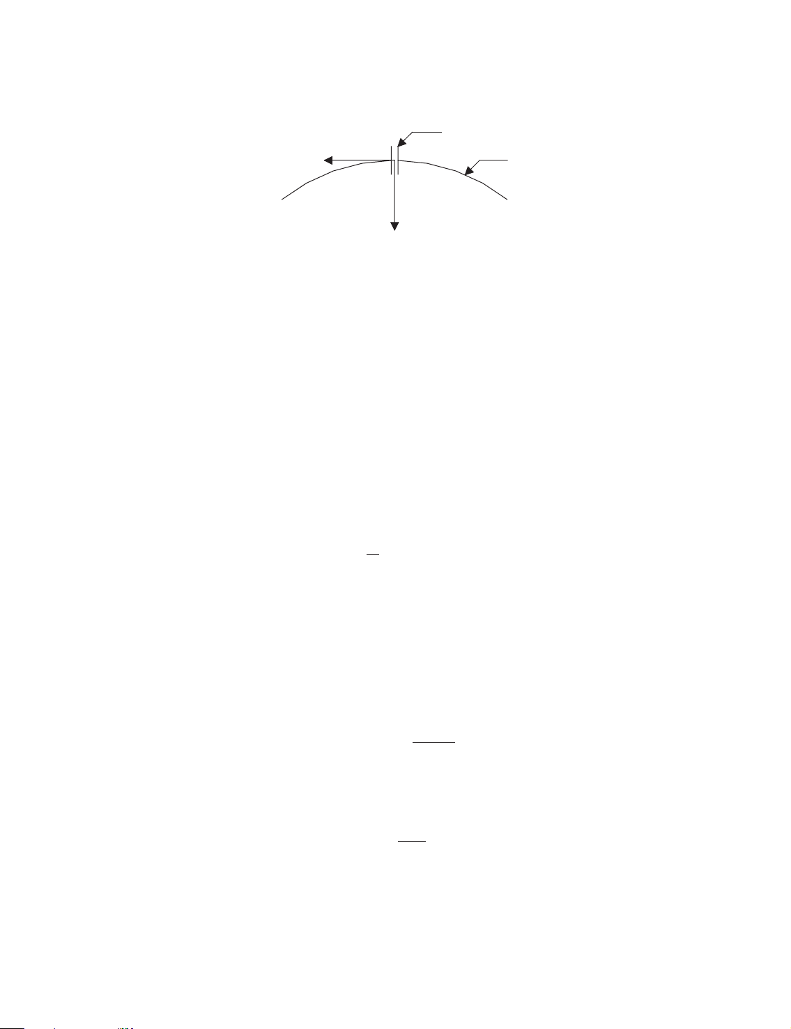
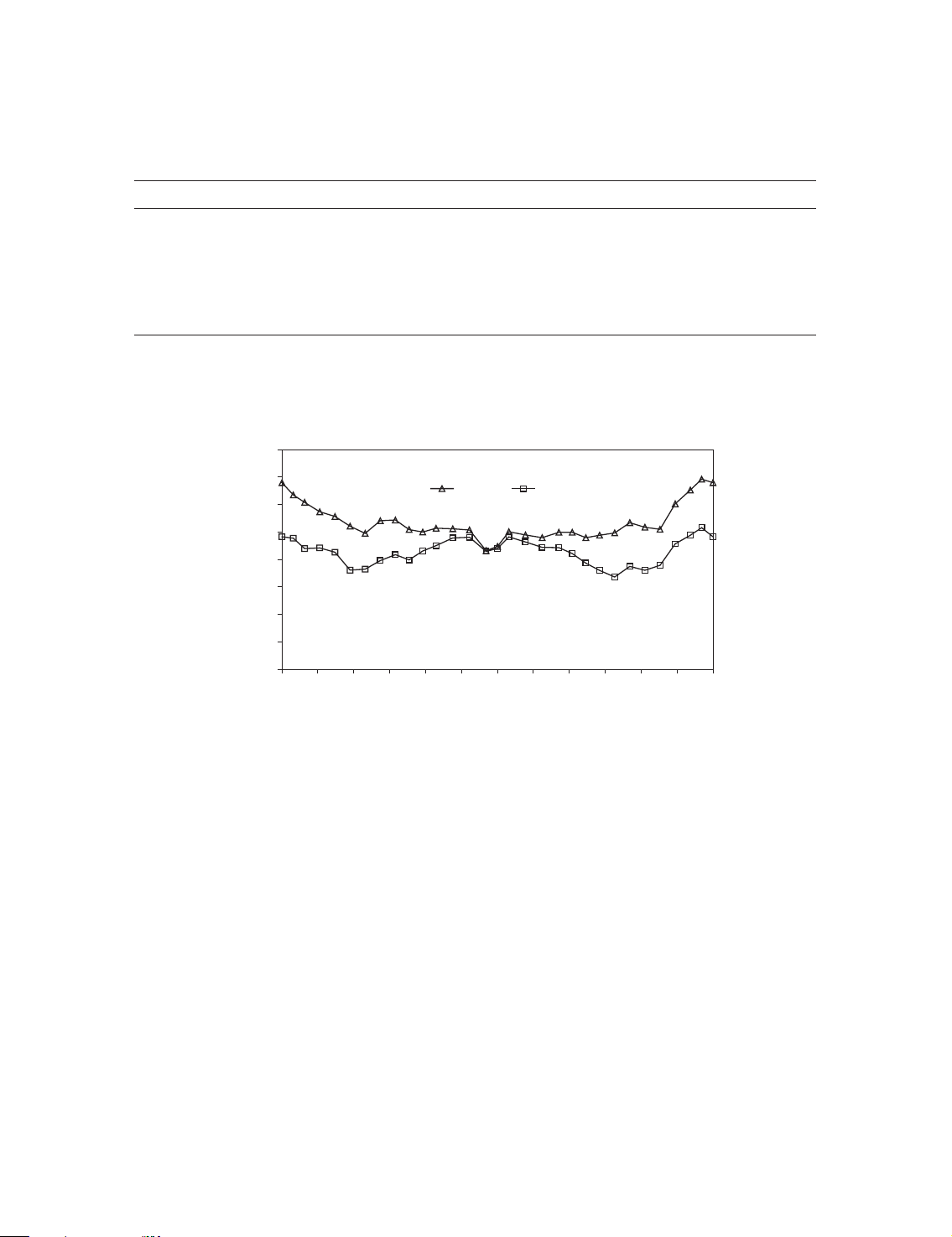
(b) Distribution of grout pressure. Two models of grout pressure distribution (Figure 8) are
considered in the analysis. The first model (GP-A) assumes that the grout pressure is uniform
and such model has the advantage of being simplicity, but, it may not be able to model the
decrease in pressure as the grout flows away from the grout hole. To overcome the above
Table II. The adopted parameters of the contact elements. Shear stiffness Normal stiffness Internal friction Cohesion Construction stage Ks ðkN=m3Þ Kn ðkN=m3Þ angle j ð8Þ c ðkPaÞ No. 1 } } } } No. 2 100 2:381 104 0.0 0.0 No. 3 1:648 105 4:286 105 20.0 100.0 No. 4 2:473 106 6:429 106 50.0 3000.0 180° Grouting hole 170° GP-A GP-B 217° 143° 232° 242° 270° 95° 90° 303° θ 19° 0 Segment joint ° 180 160 140 120 100 80 60 40 Grouting pressure (kPa) 20 0 30 60 90
120 150 180 210 240 270 300 330 360 θ (degree)
Figure 8. Grout pressure models.
Copyright # 2004 John Wiley & Sons, Ltd.
Int. J. Numer. Anal. Meth. Geomech. 2004; 28:57–91 70 W. Q. DING ET AL.
limitation, a non-uniform pressure distribution is assumed in the second model (GP-B).
Mathematically, the grout pressure at the hoop angle y is defined as y b
P ðyÞ ¼ P1 þ P2 cos ðp4y b4pÞ ð13Þ 2
where b is the grout hole angle; P1 is the pressure at y ¼ b; P2 is the pressure at y ¼ p þ b:
As two grout holes are used in the present case and they are symmetric about the vertical axis,
the non-uniform model of the grouting pressure distribution can be expressed as follows: X 2 y b P ðyÞ ¼ 2P i 1 þ P2 cos ðp4y b 2 1; y b24pÞ ð14Þ i¼1
where b1 and b2 are the grout hole angles. In the present study, P1 ¼ 5:47 kPa; P2 ¼ 77:32 kPa; b ¼ ¼ 1 1438; b2 2178:
4.7. Modelling of the stress release: stress releasing coefficient
The releasing coefficient for each construction stage is determined according to the field displacements and experience.
Depending on the degree of snaking and volume loss, the stress release coefficient is taken to
be 0.0 to 0.1 in the first stage. In the second stage, the lining structure is installed and the grout is
injected at prescribed pressure to fill up the gap between the lining and the ground. The pressure
applied will not only restrain some of the ground movements but it may cause heaving, if the
pressure is high. Consequently, the coefficient depends on the grout pressure. In the third stage,
the stress releasing is mainly caused by the gap of the shield tail, and therefore, the coefficient
will depend on the gap. In the fourth stage, it depends on the stresses that have not yet released.
The releasing coefficients for the first to the fourth construction stages are chosen to be 0.10,
0.45, 0.3 and 0.15, respectively.
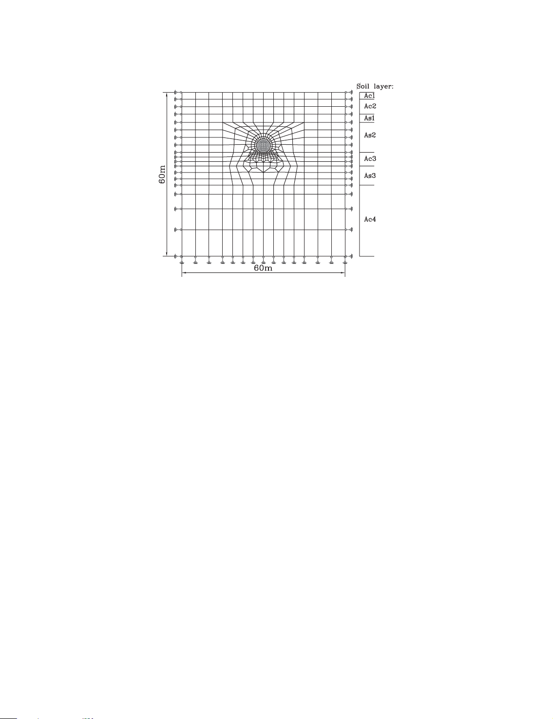
4.8. FEM mesh and boundary conditions
The initial finite element mesh adopted for the analysis is shown in Figure 9. In the finite element
simulation, the soil is modelled by 512 elements containing 545 nodes. Lining segments and their
joints are simulated with 30 beam elements and six joint elements, respectively. Thirty contact
elements are used to model the interface between the ground and lining segments. The left and
right boundaries of the mesh are laterally restricted. The bottom boundary is vertically restricted
whereas the top surface is assumed to be a free boundary. 5. RESULTS AND ANALYSIS
Section A of the Osaka No. 7 subway line is analysed in this paper and the results are compared
with the field measurement data documented in the report prepared by the Japanese Research
Society of Construction Maintenance Technique [27].
5.1. Soil displacements and settlements
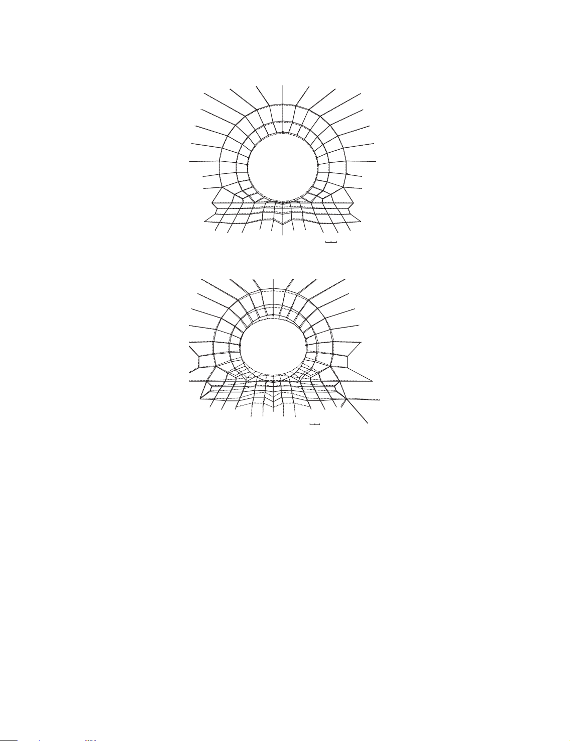
Figure 10 shows the original and deformed meshes around the shield tunnel before grouting and
after completion of Stage 4. In Table III, the displacements at four points around the tunnel are
Copyright # 2004 John Wiley & Sons, Ltd.
Int. J. Numer. Anal. Meth. Geomech. 2004; 28:57–91 ANALYSIS OF SHIELD TUNNEL 71
Figure 9. Initial finite element mesh.
tabulated. They are the results before grouting and after the completion of the Stage 4 using the
uniform grout pressure models. The settlement at the crown point A is about 7 mm: The
horizontal displacement at the points C and D are about 2–3 mm: The heave at the bottom
point B is about 11 mm: These results have shown that the soil displacements can gain
substantial increases with the progress of the construction stages.
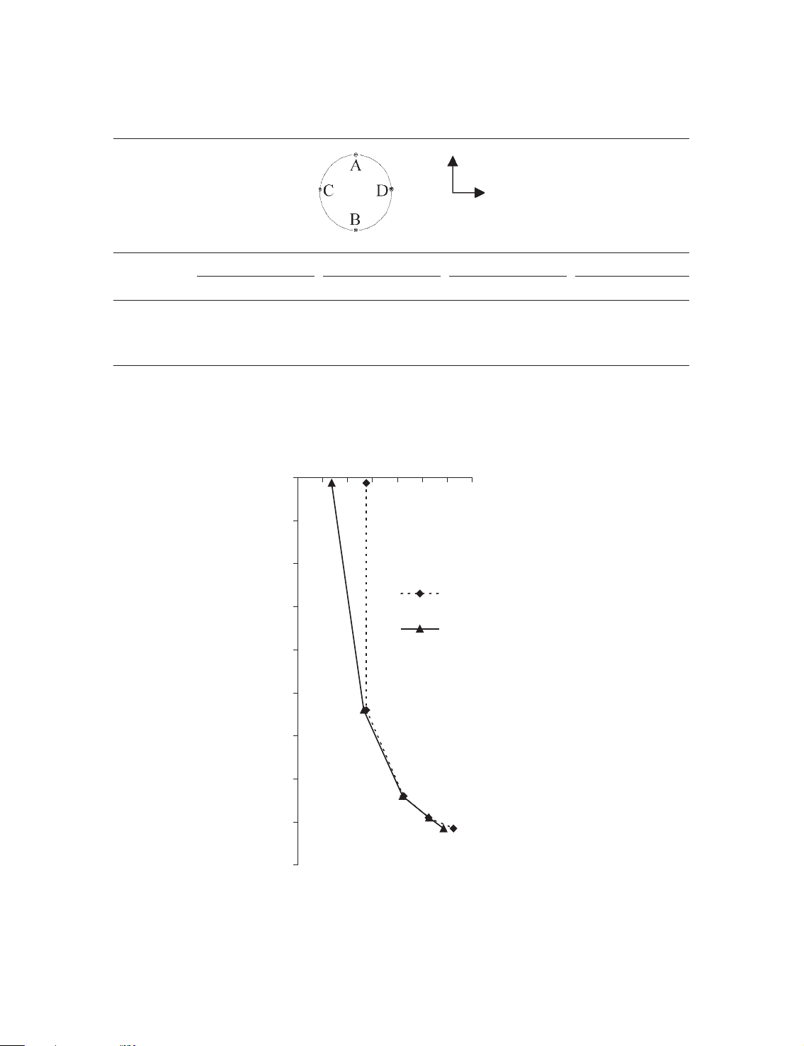
The computed settlements above the tunnel after completion of Stage 4 are compared to the
measured values in Figure 11. The results show that the computed settlements agree fairly well with the measured ones.
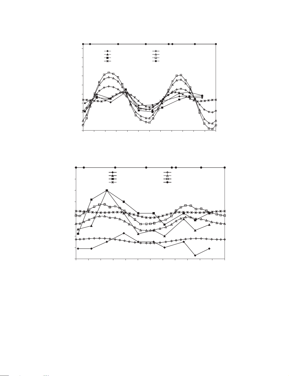
5.2. Lining bending moment, hoop force and earth pressure
Figure 12 shows the measured and computed bending moments of shield lining at the Stages 2, 3
and 4. In Figure 13, the measured and computed hoop forces of the shield lining segments are
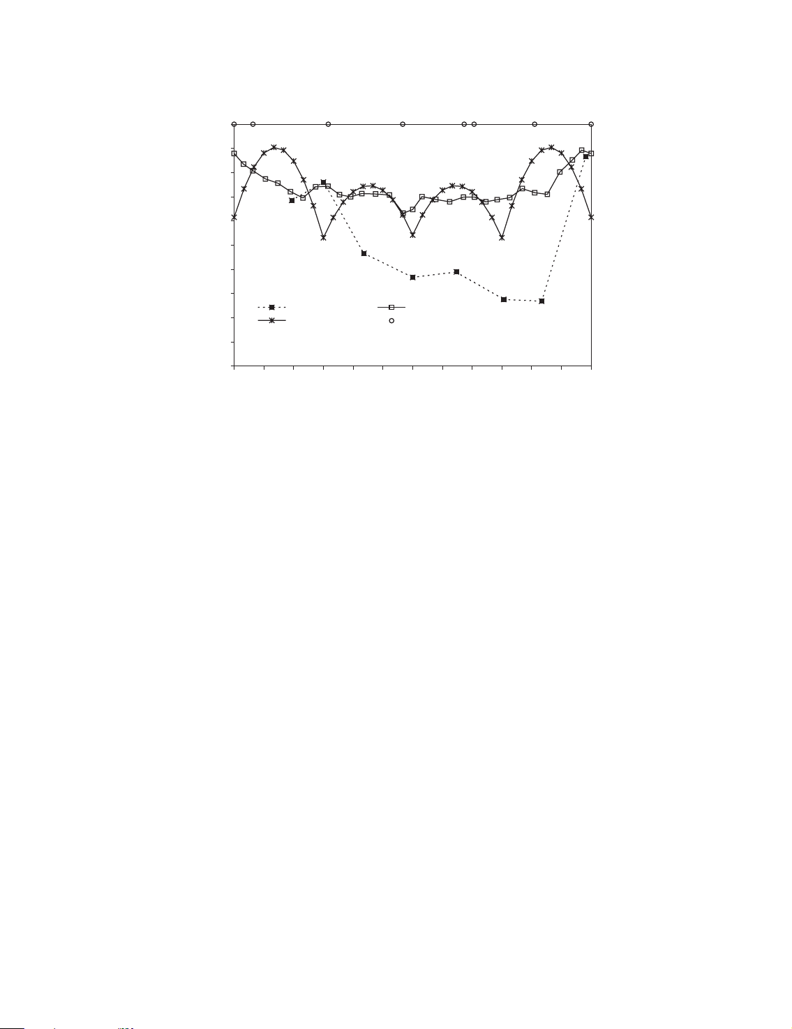
compared for the Stages 2, 3 and 4. Furthermore, the earth pressure at the Stage 4 only
is depicted in Figure 14. These results were obtained using the uniform grout pressure model
GP-A. In those figures, the corresponding predicted values using the conventional semi-
analytical design method at the Stage 4 are also presented. The conventional method is
summarized in Appendix B for an ease of reference. Details of this conventional method can be found in [10, 11, 29].
From Figure 12, it can be observed that the variations of the measured and the present FEM
predicted bending moments with respect to the hoop angle y and the construction stages are
basically similar although there are some significant discrepancies at the measurement locations
M10 ðy ¼ 758Þ and M08 ðy ¼ 3238Þ: At those two locations, the measured moments have
irregular tends with the construction stages 2–4, which indicates the measured moments might
not be correct. The absolute values of the FEM predicated moments are generally greater than
those of the measured moments. The moments predicted using the conventional method after
Copyright # 2004 John Wiley & Sons, Ltd.
Int. J. Numer. Anal. Meth. Geomech. 2004; 28:57–91 72 W. Q. DING ET AL. A C D B
Scale of total displacement from an
original point to its corresponding point: 0 20(mm) (a) A C D B
Scale of total displacement from an
original point to its corresponding point: 0 20(mm) (b)
Figure 10. Deformed meshes of around the tunnel: (a) before grouting; and (b) after completion of Stage 4.
the completion of Stage 4 are generally less than those measured values, which could cause an unsafe design.
From Figure 13, it can be observed that the variations of the measured and the present FEM
predicted hoop forces with respect to the hoop angle y and the construction stages are basically
similar although there are some significant discrepancies at the measurement locations AF01
ðy ¼ 758Þ: Basically, the hoop forces increased as the construction stage progressed, which
cannot be predicted using the conventional method. Furthermore, the measured hoop forces are
not symmetric about the vertical centre (y ¼ 0 or 1808), while the predicted results are symmetric
about the vertical axis. The percentage relative differences between each set of the measured and
FEM predicted hoop forces are between 113 and 35%. A majority of the relative differences
are within 20%: Furthermore, the predicted results using the conventional method at the
Stage 4 have the lowest variations with respect to the hoop angle y:
Copyright # 2004 John Wiley & Sons, Ltd.
Int. J. Numer. Anal. Meth. Geomech. 2004; 28:57–91 ANALYSIS OF SHIELD TUNNEL 73
Table III. The displacements of the typical points around tunnel. Point A Point B Point C Point D Construction stage Horizontal Vertical Horizontal Vertical Horizontal Vertical Horizontal Vertical 1 0 2.24 0 2.95 0.92 0.12 0.92 0.12 2 0 5.32 0.03 6.06 1.39 0.38 1.45 0.38 3 0.08 6.28 0.05 9.55 1.86 0.93 2.34 0.69 4 0.11 6.67 0.11 11.21 2.14 1.64 2.85 1.19
Note: The positive values are horizontal rightward and vertical upward; unit: mm. Settlement (mm) 0 0 1 2 3 4 5 6 7 -2 -4 Measured value -6 GP-A -8 -10 -12 -14 -16 -18 Depth (m)
Figure 11. Variation of settlement with depth.
Copyright # 2004 John Wiley & Sons, Ltd.
Int. J. Numer. Anal. Meth. Geomech. 2004; 28:57–91 74 W. Q. DING ET AL. 110 Stage 2 & measured Stage 2 & GP model A Stage 3 & measured Stage 3 & GP model A 90 Stage 4 & measured Stage 4 & GP model A Conventional design method Location of joints 70 50 30 10 -10 Bending moment (kN.m) -30 -50 -70 0 30 60 90 120 150 180 210 240 270 300 330 360 θ (degree)
Figure 12. Variation of measured and predicted bending moments with hoop angle at the
completion of construction stages 2, 3 or 4. 900 Stage 2 & measured Stage 2 & GP model A Stage 3 & measured Stage 3 & GP model A 800 Stage 4 & measured Stage 4 & GP model A Conventional design method Location of joints 700 600 500 400 300 Lining ring hoop force (kN) 200 100 0 30 60 90 120 150 180 210 240 270 300 330 360 θ (degree)
Figure 13. Variation of measured and predicted hoop forces with hoop angle at the
completion of construction stages 2, 3 or 4.
From Figure 14, it is clear that the present FEM predicted earth pressure values are very close
to those measured results at the cell Nos. EP8 ðy ¼ 588Þ; EP1 ðy ¼ 908Þ and EP7 ðy ¼ 3558Þ and
are about two times greater than those measured results at the other cell Nos. EP2 to EP6.
Furthermore, the present FEM predicted result generally decreases as the hoop angle y increases
Copyright # 2004 John Wiley & Sons, Ltd.
Int. J. Numer. Anal. Meth. Geomech. 2004; 28:57–91 ANALYSIS OF SHIELD TUNNEL 75 340 310 280 250 220 190 160 130 Normal earth pressure (kPa) Measured Present method 100 Conventional Location of joints 70 40 0 30 60 90 120 150 180 210 240 270 300 330 360 θ (degree)
Figure 14. Variation of earth pressure after completion of Stage 4.
from 0 to 1808 and then increases as the hoop angle y increases from 180 to 3608; which is
considered to be reasonable. However, the results predicted with the conventional method have
four cycles of increasing and decreasing. The four cycles correspond to the hoop angle intervals
04y5908; 9084y51808; 18084y52708 and 27084y53608; which are evidently caused by the
basic assumptions associated with the semi-analytical formation of the conventional method
(see Appendix B). Moreover, the predicted results using the conventional method are close to
those predicted using the present FEM method. The predicted results do not have significant differences.
From the above analysis and discussions, one can have the following general findings:
(a) The present method can be used to make a best prediction on the hoop forces and a
good prediction on the earth pressures and a reasonable prediction on the bending
moment. The predicted results can be used for a safe design for each of the three construction stages.
(b) The in situ measurements have a best performance for the hoop forces, a good
performance for the earth pressure and a reasonable performance for the bending
moments. There seems a need to develop more reliable senses for in situ measurement of
the bending moment in the lining.
(c) The conventional method could give a reasonably good prediction on the hoop forces,
an adequate estimation on the earth pressure and an under-estimation on the bending
moment after the completion of the Stage 4. The use of this conventional method in
design estimation of the bending moment needs a great care.
(d) These results have also shown that the mechanical responses of the shield tunnel
construction at the construction stages can be predicted by the numerical procedure
presented above. It is noted that it is very important to select correct soil parameters in the numerical prediction.
Copyright # 2004 John Wiley & Sons, Ltd.
Int. J. Numer. Anal. Meth. Geomech. 2004; 28:57–91 76 W. Q. DING ET AL.
Table IV. The relative displacements at joints of lining segment at the completion of construction stage No. 4. y 198 958 1708 2328 2428 3038 GP-A Du ðmmÞ 1.91 102 2.19 102 1.60 102 1.79 102 1.91 102 2.13 102
Dv ðmmÞ 1.62 104 9.60 104 8.54 104 1.22 105 6.15 105 1.35 103 DW ð8Þ 8.83 106 1.12 105 9.51 106 3.05 107 3.87 106 5.08 106 GP-B Du ðmmÞ 1.80 102 2.12 102 1.53 102 1.72 102 1.84 102 2.03 102
Dv ðmmÞ 1.46 104 9.01 104 8.55 104 1.66 105 5.09 105 1.42 103 DW ð8Þ 9.31 106 1.23 105 1.06 105 1.23 107 4.62 106 4.81 106
Note: Du; Dv and DW are relative normal displacement, relative shearing displacement and relative rotational angular
displacement between two nodes of joint element, respectively. 340 310 GP-A GP-B 280 250 220 190 160
Normal earth pressure (kPa) 130 100 0 30 60 90 120 150 180 210 240 270 300 330 360 θ (degree)
Figure 15. Effect of grout pressure models: earth pressure.
5.3. Joint displacement and rotation
Table IV gives the relative normal displacement, shearing displacements and rotational angular
displacements between two nodes of the joint elements after the completion of Stage 4. From
Table IV, it can be observed that the relative normal displacements vary between 0.015 and
0:022 mm: The relative shearing displacements vary between 0.000012 and 0:0014 mm: The
relative rotational angular displacements vary between 1:23 107 and 1:23 105: Such small
relative displacements at the joints can be justified by the combined factors that the joint
stiffness values (kW ¼ 2:8 108 kN m=rad=m2; kn ¼ 6:55 107 kN=m3; ks ¼ 2:5 107 kN=m3)
are much greater than those of the grout stiffness values between 100 and 6:429 106 (see
Table II), these values are close to the lining concrete bending stiffness (say, Young’s modulus/
thickness E=h ¼ 3:5 107=0:28 ¼ 1:25 108 kN=m3) in magnitude, as well as there is an
arching effect along the circular lining.
Copyright # 2004 John Wiley & Sons, Ltd.
Int. J. Numer. Anal. Meth. Geomech. 2004; 28:57–91
Tài liệu liên quan:
-

Ung dung game hoa trong cac chien dich MKT
18 9 -

Bao cao Chi so TMDT Viet Nam 2025
15 8 -
Thông tư quy định về việc phân quyền, phân cấp và phân định thẩm quyền quản lý nhà nước về giáo dục cho chính quyền địa phương
24 12 -
Nghị quyết về phát huy các giá trị di sản văn hóa gắn với phát triên du lịch bền vững tỉnh Khánh Hòa đến năm 2025, định hướng đến năm 2030
14 7 -
Quyết định phê duyệt Chiến lược phát triển du lịch Việt Nam đến năm 2030
13 7