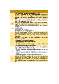
4.2.2. RESULTS OF EXPLORATORY FACTOR ANALYSIS (EFA)
With an initial study model of 4 factors and 14 observational variables, Cronbach's
Alpha results showed that the factors were acceptable, so the authors decided to include
all 51 criteria in the EFA factor analysis using Principal Component Analysis through Varimax rotation method.
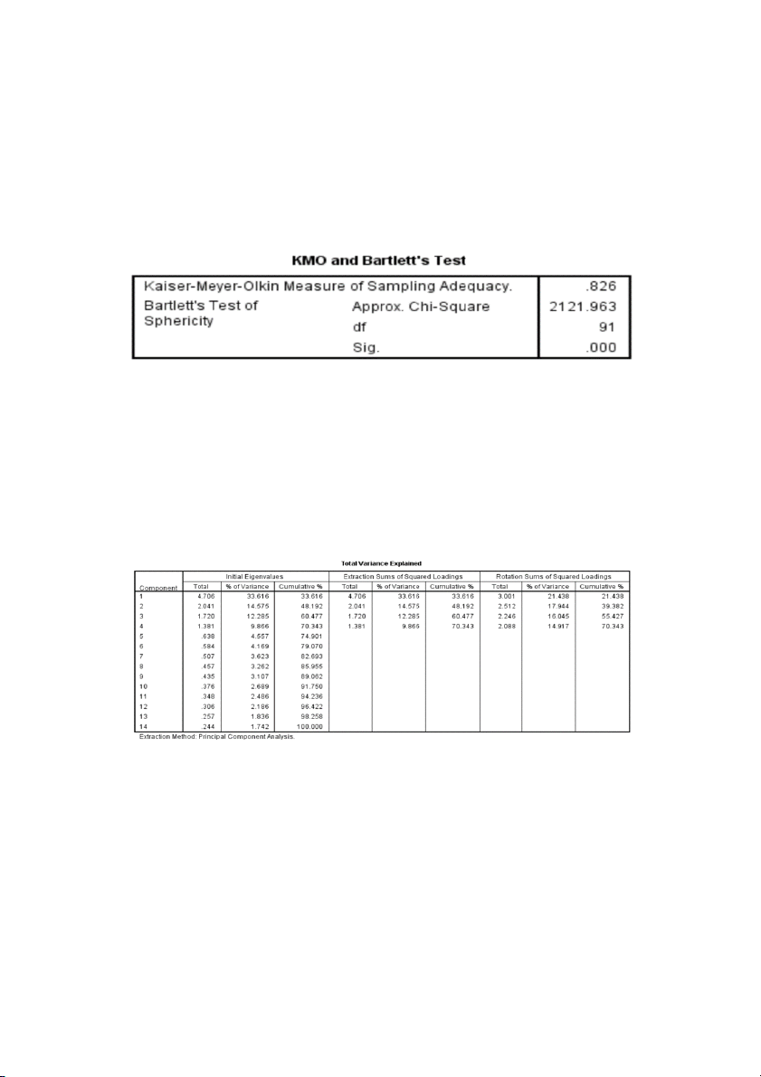
Figure 4.5. Results of KMO analysis and Bartlett's test. (Source: The authors)
 Based on Figure 4.5, the achieved KMO coefficient value is 8.26, ensuring that the
set condition (0.5 ≤ KMO ≥ 1) proves that the above discovery analysis is entirely suitable.
 The Sig Bartlett's Test achieves 0.000 < 0.05, indicates that this is a statistically
significant test, and confirms that the observed variables are correlated in the factor.
Figure 4.6. Table of results of total variance extracted. (Source: The authors)
 After running the data, the authors found four factors with Eigenvalue ≥ 1 in the
Total Variance Explained table, so the team decided to keep them in the analysis model.
 With a total variance () of 70,343%, the level is higher than the required 50%. That
reflects that 70.343% of the variability of all observed variables is included.
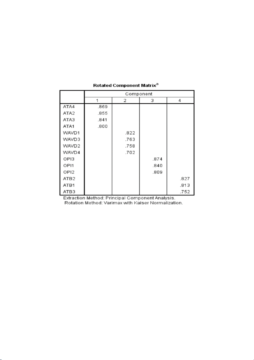
Figure 4.7. Result of the Rotated component matrix. (Source: The authors)
 The fact that the Factor Loading coefficient of the observed variables is above 0.7
demonstrates the statistical significance of the 14 elements above and the
correlation between the experimental variable and the essential factor.
 ATA4 has a higher load factor than ATA1, of 0.869, so it contributes more to the
creation of factor 1. Same with factor 2,3,4.
 There are four large groups of factors drawn after the EFA discovery factor analysis, among which:
+ Factor 1 consists of 4 observed variables, named ATA.
+ Factor 2 consists of 4 observed variables, named WAVD.
+ Factor 3 consists of 3 observed variables, named OPI.
+ Factor 4 consists of 3 observed variables, named ATB.
4.2.3. CFA INSPECTION RESULTS
 Standardized Regression Weights: (Group number 1 - Default model) Estimate ATA4 ← ATA 0.876 ATA2 ← ATA 0.817 ATA3 ← ATA 0.793 ATA1 ← ATA 0.793 WAVD1 ← WAVD 0.779 WAVD2 ← WAVD 0.667 WAVD3 ← WAVD 0.718 WAVD4 ← WAVD 0.658 OPI3 ← OPI 0.839 OPI1 ← OPI 0.767 OPI2 ← OPI 0.716 ATB2 ← ATB 0.719 ATB1 ← ATB 0.72 ATB3 ← ATB 0.755
Table 4.1. . Standardized Regression Weights results (Source: the authors)
The results from table 4.6 show that all observed variables are significant in the
scale because there are Standardized Loading Estimates greater than 0.5, most of which
are ideal when greater than 0.7.
 Correlations: (Group number 1 – Default model) Estimate ↔ ATA WAVD 0.444 ↔ ATA OPI 0.23 ↔ ATA ATB 0.391 ↔ WAVD OPI 0.225 ↔ WAVD ATB 0.457 ↔ OPI ATB 0.335
Table 4.2. Correlations analysis result. (Source: The authors)
 CR, AVE, MSV, and SQRTAVE results were calculated via Excel CR AVE MSV SQRTAVE OPI 0.819 0.602 0.112 0.776 ATA 0.892 0.673 0.197 0.820 WAVD 0.799 0.500 0.209 0.707 ATB 0.775 0.535 0.209 0.732
Table 4.3. CR, AVE, MSV, SQRTAVE results (Source: The authors)
 All CR values are more significant than 0.7, thanks to which scale reliability is guaranteed.
 AVE values are all greater than 0.5, ensuring convergence.
 Differentiation is guaranteed when all MSV values are less than AVE and
SQRTAVE values are more significant than all Inter-Construct Correlations.
4.2.4 SEM LINEAR STRUCTURE MODEL EVALUATION
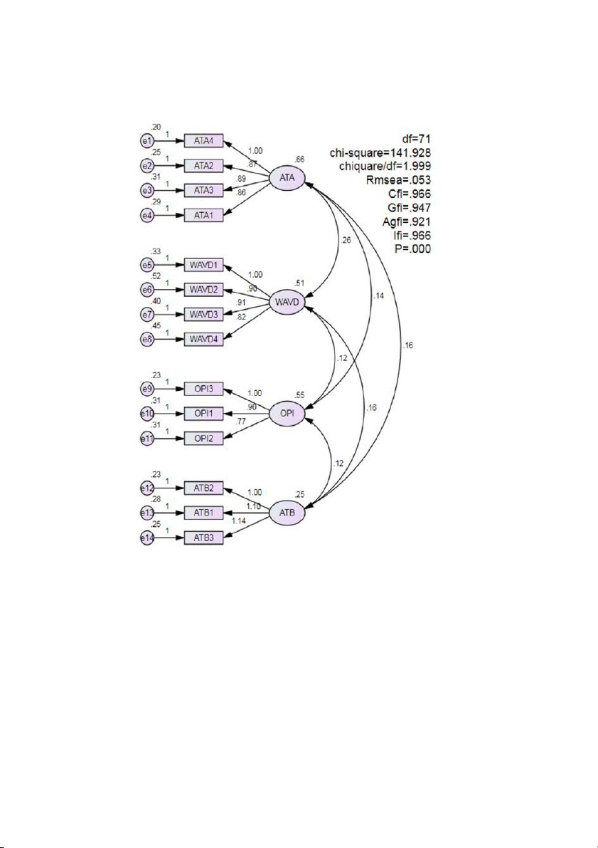
Figure 4.8. CFA analysis results. (Source: The authors)
After calculating the correlation between error and observed variables, the CFA
results showed that the model had 71 degrees of freedom. The genus – square is 141,928
(p = 0.000). A CFI value = 0.966 indicates that the model is moderate (TLI, CFI > 0.9),
and a Chisquare value / df = 1.999 indicates that the model is highly statistically
significant. Besides, the RMSEA value = 0.053 indicates that the model is also good
enough to use (CMIN < 3, RMSEA < 0.08), meeting the required standard. Therefore, the
prediction model is accurate and consistent with market data.
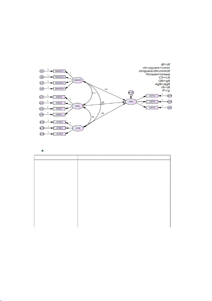
4.2.5 HYPOTHESIS EVALUATION THROUGH SEM ANALYSIS Figure 4.9. Model SEM
Regression Weights: (Group number 1 - Default model) Estimate S.E. C.R. P Label OPI ← WAVD 0.059 0.082 0.725 0.468 H3 OPI ← ATA 0.091 0.065 1.4 0.161 H5 OPI ← ATB 0.402 0.119 3.383 *** H6 ATA4 ← ATA 1 ATA2 ← ATA 0.869 0.047 18.589 *** ATA3 ← ATA 0.891 0.05 17.794 *** ATA1 ← ATA 0.863 0.049 17.772 *** WAVD1 ← WAVD 1 WAVD2 ← WAVD 0.9 0.079 11.33 *** WAVD3 ← WAVD 0.913 0.076 12.075 *** WAVD4 ← WAVD 0.824 0.074 11.19 *** OPI3 ← OPI 1 OPI1 ← OPI 0.897 0.069 13.011 *** OPI2 ← OPI 0.773 0.062 12.508 *** ATB2 ← ATB 1 ATB1 ← ATB 1.101 0.101 10.873 *** ATB3 ← ATB 1.144 0.103 11.074 ***
Table 4.4. Regression Weights of the research.
Covariances: (Group number 1 - Default model) Estimate S.E. C.R. P Label ATA ↔ WAVD 0.258 0.041 6.28 *** H1 WAVD ↔ ATB 0.163 0.028 5.829 *** H2 ATA ↔ ATB 0.159 0.029 5.479 *** H4
Table 4.5. Covariances of the research. Inspection results
According to the 95% reliability standard, WAVD's sig affects an OPI equals
0.468> 0.05, so the WAVD variable does not affect OPI; the sig’s impact of ATA is
0.161> 0.05 indicates that the ATA variable does not affect OPI either. The remaining
variables all have sig equal to 0.000 (AMOS sign *** is sig equal to 0.000), as a result,
these relationships are meaningful. In fact, we found there are pairs of variables that
affect each other - ATA and ATB, ATA and WAVD, and WAVD and ATB. And we also
found that the OPI variable has a specific impact on ATB. Along with that, we reject the
H3, and H5 hypotheses; while the rest of them is accepted, according to the following table:
H1: Visual design of Web advertising (WAVD) will positively affect the Attitude
towards advertising (ATA). (p > 0.05). Hypothesis H1 is supported
H2: Product risk will have a positive impact on the Attitude toward online shopping (p
< 0.05). Hypothesis H2 is supported
H3: Web advertising visual design (WAVD) will have a good effect on the Attitude
towards brand (ATB) (p > 0.05). Hypothesis H3 is rejected
H4: Attitude towards web advertising (ATA) will influence the Attitude towards brands
(ATB). (p < 0.05). Hypothesis H4 is supported
H5: Attitude towards web advertising (ATA) will positively impact online purchase
intention (OPI). (p > 0.05). Hypothesis H5 is rejected
H6 Attitude towards brand (ATB) will have a good impact on online purchase intention
(OPI) (p < 0.05). Hypothesis H6 is supported
Table 4.11. Hypotheses used in the study.
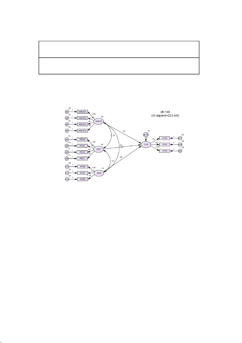
4.2.6 MODERATING EFFECT ANALYSIS RESULTS Invariant model:
Figure 4.1. Invariant model of the research Variable model:
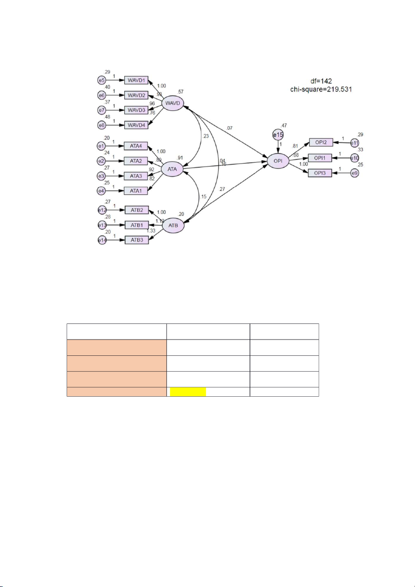
Figure 4.11. Variable model of the research.
These two invariant and variable models are built through Amos. The test results
obtained Chi-square and df values representing a meaningful relationship between the
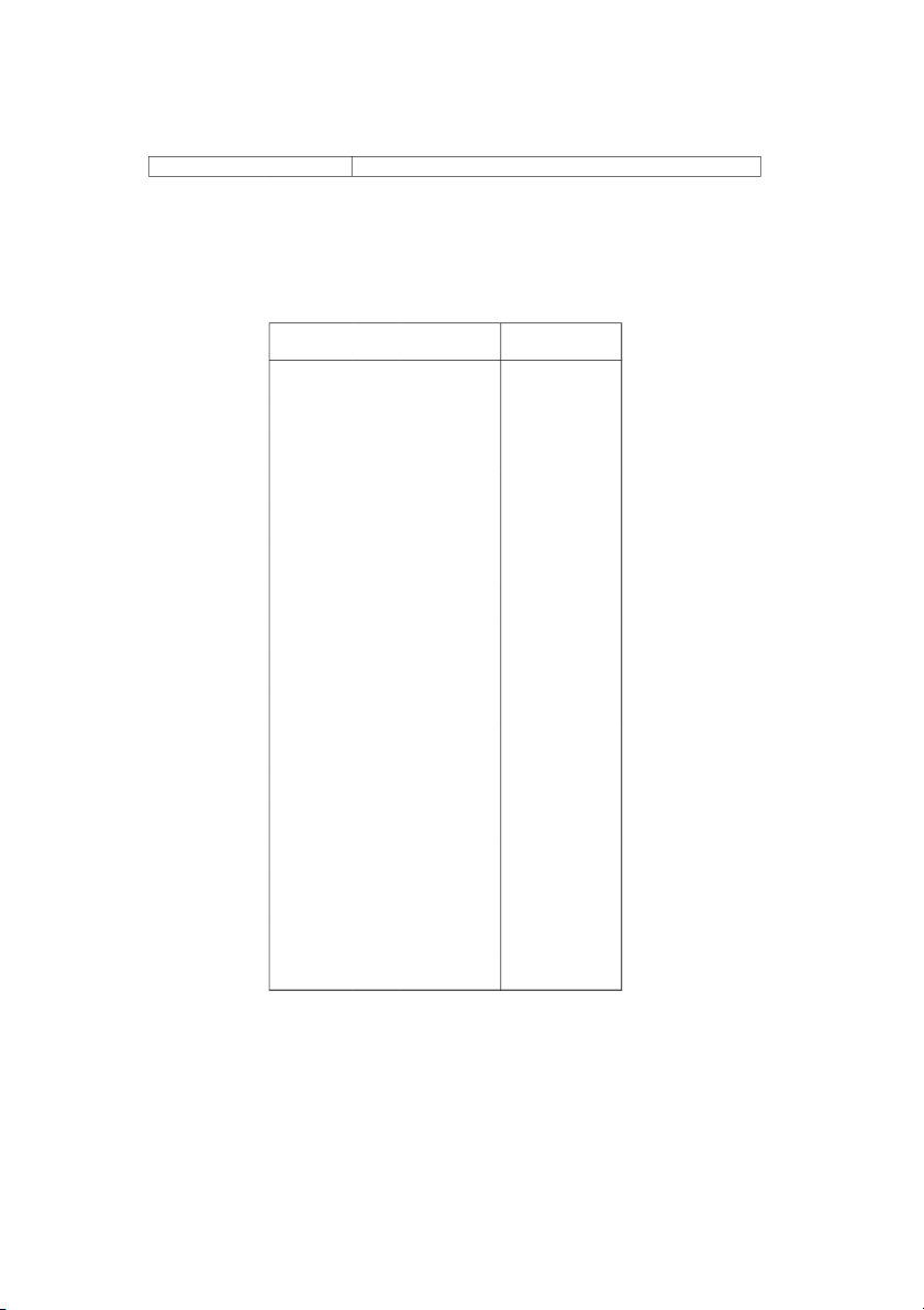
two variables, which is used to calculate the P-value, according to the following table: Chi-square df Invariant 223.606 148 Variable 219.531 142 Discrepancy 4.075 6 P-value 0.66652745
Table 4.12. P-value results.
Since the P-value reaches 0.67 > 0.05 (95% confidence), neither model has a Chi-
square difference. The authors accepted the H0 hypothesis, choosing an invariant model to explain the results. Estimate S.E. C.R. P Label OPI ← ATA 0.087 0.065 1.35 0.177 H5 OPI ← ATB 0.436 0.119 3.661 *** H6 OPI ← WAVD 0.055 0.082 0.667 0.505 H3 ATA4 ← ATA 1 ATA2 ← ATA 0.889 0.056 15.942 *** ATA3 ← ATA 0.922 0.059 15.747 *** ATA1 ← ATA 0.815 0.054 15.137 *** WAVD1 ← WAVD 1 WAVD2 ← WAVD 0.925 0.097 9.53 *** WAVD3 ← WAVD 0.965 0.098 9.853 *** WAVD4 ← WAVD 0.761 0.094 8.087 *** OPI3 ← OPI 1 OPI1 ← OPI 0.852 0.099 8.562 *** OPI2 ← OPI 0.794 0.092 8.585 *** ATB2 ← ATB 1 ATB1 ← ATB 1.16 0.165 7.03 *** ATB3 ← ATB 1.389 0.186 7.469 ***
Table 4.13. Regression Weights: (Male -Default model) Estimate S.E. C.R. P Label OPI ← ATA 0.087 0.065 1.35 0.177 H5 OPI ← ATB 0.436 0.119 3.661 *** H6 OPI ← WAVD 0.055 0.082 0.667 0.505 H3 ATA4 ← ATA 1 ATA2 ← ATA 0.843 0.082 10.235 *** ATA3 ← ATA 0.847 0.088 9.597 *** ATA1 ← ATA 0.95 0.092 10.38 *** WAVD1 ← WAVD 1 WAVD2 ← WAVD 0.888 0.121 7.32 *** WAVD3 ← WAVD 0.884 0.109 8.125 *** WAVD4 ← WAVD 0.899 0.111 8.066 *** OPI3 ← OPI 1 OPI1 ← OPI 0.939 0.094 9.983 *** OPI2 ← OPI 0.758 0.082 9.195 *** ATB2 ← ATB 1 ATB1 ← ATB 1.075 0.122 8.812 *** ATB3 ← ATB 1.045 0.119 8.815 ***
Table 4.14. Regression Weights: (Female - Default model).
The p-value for the effects in both Male and Female groups are the same. There is
no significant difference between the effects of ATA and WAVD on OPI, but still has
some meanings among the remaining. Estimate OPI ← ATA 0.114 OPI ← ATB 0.256 OPI ← WAVD 0.056 ATA4 ← ATA 0.906 ATA2 ← ATA 0.868 ATA3 ← ATA 0.863 ATA1 ← ATA 0.846 WAVD1 ← WAVD 0.817 WAVD2 ← WAVD 0.744 WAVD3 ← WAVD 0.769 WAVD4 ← WAVD 0.642 OPI3 ← OPI 0.837 OPI1 ← OPI 0.736 OPI2 ← OPI 0.739 ATB2 ← ATB 0.637 ATB1 ← ATB 0.691 ATB3 ← ATB 0.809
Table 4.15. Standardized Regression Weights: (Male - Default model) Estimate ← OPI ATA 0.076 ← OPI ATB 0.316 ← OPI WAVD 0.049 ← ATA4 ATA 0.817 ← ATA2 ATA 0.734 ← ATA3 ATA 0.693 ← ATA1 ATA 0.744 ← WAVD1 WAVD 0.737 ← WAVD2 WAVD 0.605 ← WAVD3 WAVD 0.68 ← WAVD4 WAVD 0.674 ← OPI3 OPI 0.837 ← OPI1 OPI 0.796 ← OPI2 OPI 0.698 ← ATB2 ATB 0.769 ← ATB1 ATB 0.734 ← ATB3 ATB 0.734
Table 4.16. Standardized Regression Weights: (Female - Default model)
There are major differences in Standard regression weights of the impact between
the male and female groups, reflecting the degree of influence of the variable on the
group as a whole. For example, the effect of ATB on OPI in the male group was 25.6%,
while in the female group, it was higher, reaching 31.6%. The results show that women
are more likely to be influenced by a brand's personality when making purchasing
decisions than men. The following indicators are similar.
The R-squared correlation value shows an impact between the genders, but the
degree of influence between the relationships differs. According to chapter 2, section
2.1.4, hypotheses H7a, H7b, H7c, H7d, H7e, and H7f have been proposed. The
hypotheses testing has led to the following conclusions:
H7a: The effect of Web advertising visual design (WAVD) on Attitudes towards
advertising (ATA) is stronger in men than in women. Refutation of the hypothesis (0.352<0.598).
H7b: Web advertising visual design (WAVD) influence brand attitudes (ATB) is more
potent in men than in women. Accept the hypothesis (0.483>0.447)
H7c: The impact of Web advertising visual design (WAVD) on online purchase intent
(OPI) in males is stronger than in females. The hypothesis is acceptable (0.056>0.049)
H7d: The effect of Attitudes towards advertising (ATA) on Attitudes towards brands
(ATB) is stronger in men than in women. Reject the hypothesis (0.363<0.442).
H7e: The effect of Attitudes towards advertising (ATA) on Online purchase intent (OPI)
is stronger in men than in women. Hypothetical acceptance (0.114>0.076)
H7f: The effect of brand attitude (ATB) on online purchase intent (OPI) in men is
stronger than in women. The hypothesis is rejected (0.256<0.316).
Table 4.17. The results of the hypotheses in the research paper. 4.2.7 CHAPTER SUMMARY
Chapter 4 discusses the results of using descriptive statistics, reliability testing
using Cronbach's Alpha, and discovery factor analysis (EFA) to explore relationships
between variables. From there, comment on the model's compatibility with the proposed hypotheses.
The results of the SEM linear structure model show the impact of variables and
remove some links since no influence is necessary. The authors discovered that Brand
attitude was the most important factor influencing purchase intentions (estimate: 0.402).
The mutual impact of the Attitudes towards advertising (ATAs) and the Visual design of
web advertising is 0.258. The interplay of the Visual Design variables of web advertising
and Attitude toward brand (ATB) is 0.163. Finally, the weakest impress, with a value of
0.159, is the Changing attitude towards the visual design of brands and Web advertising.
Having continued to test the hypotheses, the authors accept the H1, H2, H4, H6
hypotheses. The remaining hypotheses H3, H5, H6 are rejected.
The authors then went on to test the Moderating effect and noticed that the result
would vary depending on gender. The influence of Web advertising visual design
(WAVD) on Attitude toward brand (ATB) in men was more potent than in women,
reaching a peak value of 0.483. The second is that Attitudes toward advertisements
(ATAs) substantially influence men's online purchase intention (OPI) more than women's,
at 0.114. At the lowest level, the influence of Web advertising visual design (WAVD) on
Online purchase intention (OPI) in men is more potent than in women. This number was
found to be 0.056. So, the following hypotheses are accepted: H7b, H7c, H7e. The
remaining hypotheses H7a, H7d, and H7f are all rejected.