
Downloaded by v ng (ngttgi20804@gmail.com)
CFA Level 1 All Formulas
Post Graduate Diploma in management (Rajagiri Business School)
Downloaded by v ng (ngttgi20804@gmail.com)
Copyright © 2017 by John Wiley & Sons, Inc. All rights reserved.
Published by John Wiley & Sons, Inc., Hoboken, New Jersey.
Published simultaneously in Canada.
No part of this publication may be reproduced, stored in a retrieval system, or transmitted in any
form or by any means, electronic, mechanical, photocopying, recording, scanning, or otherwise,
except as permitted under Section 107 or 108 of the 1976 United States Copyright Act, without
either the prior written permission of the Publisher, or authorization through payment of the
appropriate per-copy fee to the Copyright Clearance Center, Inc., 222 Rosewood Drive, Danvers,
MA 01923, (978) 750-8400, fax (978) 646-8600, or on the Web at www.copyright.com. Requests
to the Publisher for permission should be addressed to the Permissions Department, John Wiley &
Sons, Inc., 111 River Street, Hoboken, NJ 07030, (201) 748-6011, fax (201) 748-6008, or online
at http://www.wiley.com/go/permissions.
Limit of Liability/Disclaimer of Warranty: While the publisher and author have used their best
efforts in preparing this book, they make no representations or warranties with respect to the
accuracy or completeness of the contents of this book and specifically disclaim any implied
warranties of merchantability or fitness for a particular purpose. No warranty may be created or
extended by sales representatives or written sales materials. The advice and strategies contained
herein may not be suitable for your situation. You should consult with a professional where
appropriate. Neither the publisher nor author shall be liable for any loss of profit or any other
commercial damages, including but not limited to special, incidental, consequential, or other
damages.
For general information on our other products and services or for technical support, please contact
our Customer Care Department within the United States at (800) 762-2974, outside the United
States at (317) 572-3993 or fax (317) 572-4002.
Wiley publishes in a variety of print and electronic formats and by print-on-demand. Some
material included with standard print versions of this book may not be included in e-books or in
print-on-demand. If this book refers to media such as a CD or DVD that is not included in the
version you purchased, you may download this material at http://booksupport.wiley.com. For
more information about Wiley products, visit www.wiley.com.
QUANTITATIVe MeTHODs
FV
N
= PV (1 + r)
N
PV =
FV
(1 + r)
N
PV
Annuity Due
= PV
Ordinary Annuity
(1 + r)
FV
Annuity Due
= FV
Ordinary Annuity
(1 + r)
PV(perpetuity) =
PMT
I/Y
FV
N
= PVe
r
s
N
EAR = (1 + Periodic interest rate)
N
1
THE TIME VALUE OF MONEY
T
H
e T
I
me V
A
l
U
e of Mone
Y
The Future Value of a Single Cash Flow
The Present Value of a Single Cash Flow
Present Value of a Perpetuity
Continuous Compounding and Future Values
Effective Annual Rates
© Wiley 2017
All Rights
Reserved.
Any unauthorized
copying
or distribution
will
constitute an
infringement
of copyright.
ghts Reserved. Any unauthorized copying or distribution will constitute an infringement of co
N
NPV =
t=0
CF
t
1 + r)
t
t
F
BD
=
D
360
r
HPY =
P
1
P
0
+ D
1
=
P
1
+ D
1
1
P
0
P
0
EAY = (1 + HPY)
365/t
1
HPY = (1 + EAY)
t/365
1
DISCOUNTED CASH FLOW APPLICATIONS
D
I
sco
UNT
ed C
A
s
H
Flow A
PP
l
ICATION
s
Net Present Value
where:
CF
t
= the expected net cash flow at time t
N = the investment’s projected life
r = the discount rate or appropriate cost of capital
Bank Discount Yield
where:
r
BD
= the annualized yield on a bank discount basis
D = the dollar discount (face value purchase price)
F = the face value of the bill
t = number of days remaining until maturity
Holding Period Yield
where:
P
0
= initial price of the investment.
P
1
= price received from the instrument at maturity/sale.
D
1
= interest or dividend received from the investment.
Effective Annual Yield
where:
HPY = holding period yield
t = numbers of days remaining till maturity
360 (t r
BD
)
MM
360 r
BD
R =
R
MM
= HPY (360/t)
BEY = [(1 + EAY)
0.5
1] 2
DISCOUNTED CASH FLOW APPLICATIONS
Money Market Yield
Bond Equivalent Yield
© Wiley 2017
All Rights
Reserved.
Any unauthorized
copying
or distribution
will
constitute an
infringement
of copyright.
ghts Reserved. Any unauthorized copying or distribution will constitute an infringement of co
=
i=1
x
i
N
N
X =
i=1
x
i
n
n
1 + R
G
=
T
(1 + R
1
) (1 + R
2
) (1 + R
T
) OR G =
n
X
1
X
2
X
3
X
n
with X
i
0 fori = 1, 2,
, n.
1
R
G
=
(1 + R
t
)
1
T
T
t=1
Harmonic mean: X
H
=
N
x
N
1
with X 0 for i = 1,2,,N.
i
i=1
i
L
y
=
(
n
+
1
)y
100
Range = Maximum value Minimum value
STATISTICAL
CONCEPTS
S
TATI
s
TICA
l
Conce
PT
s
Population Mean
where:
x
i
= is the ith observation.
Sample Mean
Geometric Mean
Harmonic Mean
Percentiles
where:
y = percentage point at which we are dividing the distribution
L
y
= location (L) of the percentile (P
y
) in the data set sorted in ascending order
Range
X
i
X
n
n
2
=
i=1
(X
i
)
2
N
N
=
(X
i
)
2
i=1
N
N
(X
i
X)
2
n
n 1
s =
(X
i
X)
2
i=1
n 1
n
STATISTICAL
CONCEPTS
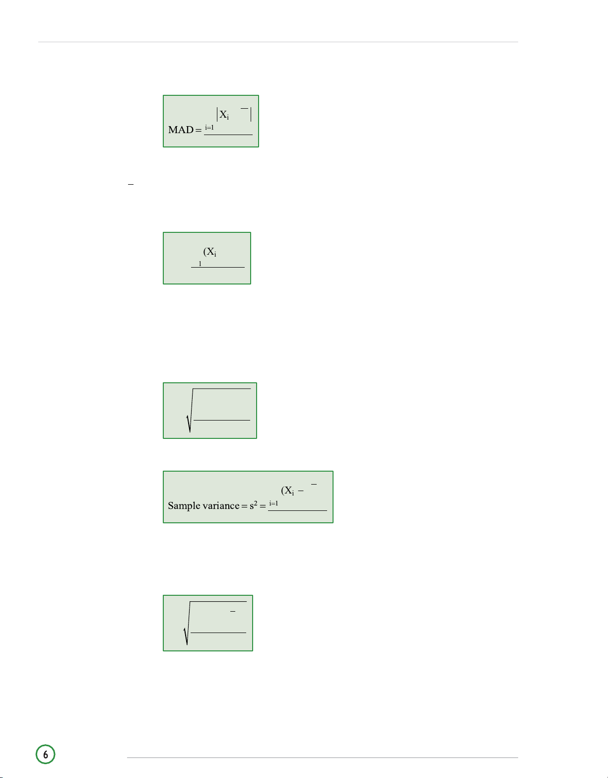
Mean Absolute Deviation
where:
n = number of items in the data set
X = the arithmetic mean of the sample
Population Variance
where:
X
i
= observation i
μ = population mean
N = size of the population
Population Standard Deviation
Sample Variance
where:
n = sample size.
Sample Standard Deviation
© Wiley 2017
All Rights
Reserved.
Any unauthorized
copying
or distribution
will
constitute an
infringement
of copyright.
ghts Reserved. Any unauthorized copying or distribution will constitute an infringement of co
Coefficient of variation =
s
X
Sharpe ratio =
r
p
r
f
s
p
S
=
n
K
(n 1)(n 2)
i=1
(X
i
X)
3
n
s
3
(X
i
X)
3
n
S
K
1
i=
1
n
s
3
3(n 1)
2
(n 2)(n 3)
4
s
(n 1)(n 2)(n 3)
i=1
n
(X
i
X)
n(n + 1)
K
E
=
STATISTICAL
CONCEPTS
Coefficient of Variation
where:
s = sample standard deviation
X = the sample mean.
Sharpe Ratio
where:
r
p
= mean portfolio return
r
f
= risk‐free return
s
p
= standard deviation of portfolio returns
Sample skewness, also known as sample relative skewness, is calculated as:
As n becomes large, the expression reduces to the mean cubed deviation.
where:
s = sample standard deviation
Sample Kurtosis uses standard deviations to the fourth power. Sample excess kurtosis is
calculated as:
K
E
1
i=1
(X
i
X)
4
n
n
s
4
3
STATISTICAL
CONCEPTS
As n becomes large the equation simplifies to:
where:
s = sample standard deviation
For a sample size greater than 100, a sample excess kurtosis of greater than 1.0 would be
considered unusually high. Most equity return series have been found to be leptokurtic.
© Wiley 2017
All Rights
Reserved.
Any unauthorized
copying
or distribution
will
constitute an
infringement
of copyright.
ghts Reserved. Any unauthorized copying or distribution will constitute an infringement of co
P(E) =
a
(a + b)
P(E) =
b
(a + b)
P(A B) =
P(AB)
given that P(B) 0
P(B)
P(AB) = P(A B) P(B)
P(A or B) = P(A) + P(B) P(AB)
P(A B) =
P(A), or equivalently, P(B A)
= P(B)
P(A or B)
= P(A) + P(B) P(AB)
P(A and B) = P(A) P(B)
P(A)
= P(AS) + P(AS
c
)
P(A) = P(A S) P(S) + P(A S
c
) P(S
c
)
P(A) =
P(A S
1
)
P(S
1
)
+
P(A S
2
)
P(S
2
)
++
P(A S
n
)
P(S
n
)
where the set of events {S
1
, S
2
,, S
n
} is mutually exclusive and exhaustive.
PROBABILITY
CONCEPTS
P
ROBABI
l
ITY
Conce
PT
s
Odds for an Event
Where the odds for are given as “a to b”, then:
Odds for an Event
Where the odds against are given as “a to b”, then:
Conditional Probabilities
Multiplication Rule for Probabilities
Addition Rule for Probabilities
For Independant Events
The Total Probability Rule
The Total Probability Rule for n Possible Scenarios
E(X) = P(X
1
)X
1
+ P(X
2
)X
2
+
P(X
n
)X
n
E(X)
=
P(X
i
)X
i
i=1
n
2
(X) = E{[X E(X)]
2
}
2
(X) =
P(X
i
) [X
i
E(X)]
2
i=1
n
Cov(XY) = E{[X E(X)][Y E(Y)]}
Cov(R
A
,R
B
) = E{[R
A
E(R
A
)][R
B
E(R
B
)]}
Corr(R ,R ) = (R ,R ) =
Cov(R ,R )
A B
A B
A B
(
A
)(
B
)
PROBABILITY
CONCEPTS
Expected Value
where:
X
i
= one of n possible outcomes.
Variance and Standard Deviation
The Total Probability Rule for Expected Value
1. E(X) = E(X
|
S)P(S) + E(X
|
S
c
)P(S
c
)
2. E(X) = E(X
|
S
1
) × P(S
1
) + E(X
|
S
2
) × P(S
2
) + . . . + E(X
|
S
n
) × P(S
n
)
where:
E(X) = the unconditional expected value of X
E(X
|
S
1
) = the expected value of X given Scenario 1
P(S
1
) = the probability of Scenario 1 occurring
The set of events {S
1
, S
2
, . . . , S
n
} is mutually exclusive and exhaustive.
Covariance
Correlation Coefficient
© Wiley 2017
All Rights
Reserved.
Any unauthorized
copying
or distribution
will
constitute an
infringement
of copyright.
ghts Reserved. Any unauthorized copying or distribution will constitute an infringement of co
E(R
p
) =
w
i
E(R
i
) = w
1
E(R
1
) + w
2
E(R
2
) ++ w
N
E(R
N
)
i=1
N
Var(R
p
) =

w
i
w
j
Cov(R
i
,R
j
)
i=1 j=1
N N
A A B B
A B
A B
A A B B
A B A B A B
A A B B C C
+ 2w
A
w
B
Cov(R
A
,R
B
) + 2w
B
w
C
Cov(R
B
,R
C
) + 2w
C
w
A
Cov(R
C
,R
A
)
P(Event Information) =
P (Information Event) P (Event)
P (Information)
n r
C =
n
=
r
n!
(n r)!(r!)
PROBABILITY
CONCEPTS
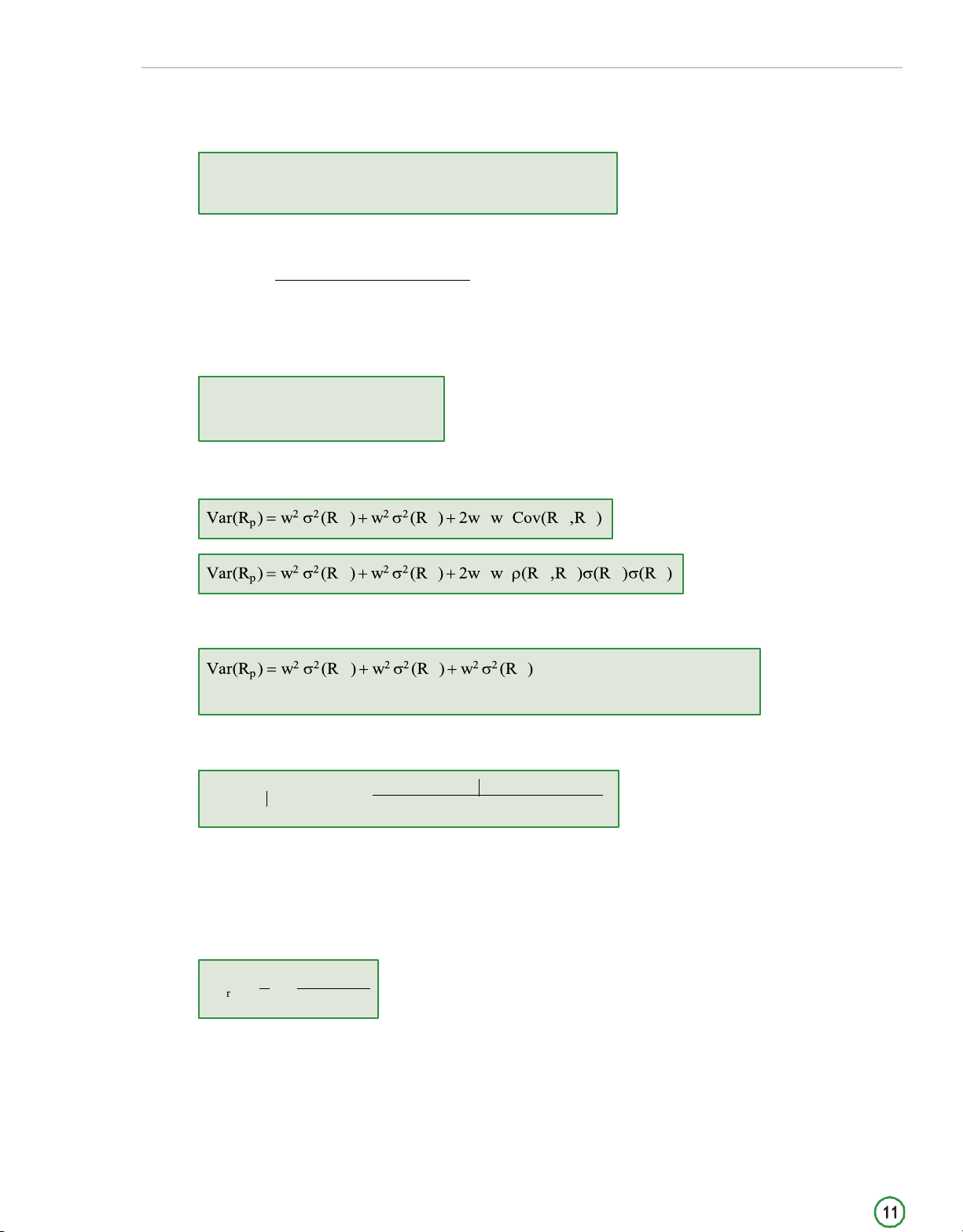
Expected Return on a Portfolio
where:
Weight of asseti =
Market value of investment i
Market value of portfolio
Portfolio Variance
Variance of a 2 Asset Portfolio
Variance of a 3 Asset Portfolio
Bayes’ Formula
Counting Rules
The number of different ways that the k tasks can be done equals n
1
n
2
n
3
n
k
.
Combinations
Remember: The combination formula is used when the order in which the items are
assigned the labels is NOT important.
Permutations
F(x) = n p(x) for the nth observation.
P(X=x) =
n
C
x
(p)
x
(1 p)
n-x
2
= n p (1 p)
x
Tracking error = Gross return on portfolio Total return on benchmark index
P(X a), P (X b) = 0
P (x X x ) =
x x
2 1
1
2
b a
COMMON
PROBABILITY
DISTRIBUTIONS
Common PROBABIlITY DIsTRIBUTIONs
Discrete Uniform Distribution
Binomial Distribution
where:
p = probability of success
1 p = probability of failure
n
C
x
= number of possible combinations of having x successes in n trials. Stated differently,
it is the number of ways to choose x from n when the order does not matter.
Variance of a Binomial Random Variable
Tracking Error
The Continuous Uniform Distribution
Confidence Intervals
For a random variable X that follows the normal distribution:
The 90% confidence interval is x 1.65s to x + 1.65s
The 95% confidence interval is x 1.96s to x + 1.96s
The 99% confidence interval is x 2.58s to x + 2.58s
The following probability statements can be made about normal distributions
Approximately 50% of all observations lie in the interval μ ± (2/3)σ
Approximately 68% of all observations lie in the interval μ ± 1σ
Approximately 95% of all observations lie in the interval μ ± 2σ
Approximately 99% of all observations lie in the interval μ ± 3σ

Preview text:

CFA Level 1 All Formulas
Post Graduate Diploma in management (Rajagiri Business School)
Downloaded by v ng (ngttgi20804@gmail.com)
Copyright © 2017 by John Wiley & Sons, Inc. All rights reserved.
Published by John Wiley & Sons, Inc., Hoboken, New Jersey.
Published simultaneously in Canada.
No part of this publication may be reproduced, stored in a retrieval system, or transmitted in any
form or by any means, electronic, mechanical, photocopying, recording, scanning, or otherwise,
except as permitted under Section 107 or 108 of the 1976 United States Copyright Act, without
either the prior written permission of the Publisher, or authorization through payment of the
appropriate per-copy fee to the Copyright Clearance Center, Inc., 222 Rosewood Drive, Danvers,
MA 01923, (978) 750-8400, fax (978) 646-8600, or on the Web at www.copyright.com. Requests
to the Publisher for permission should be addressed to the Permissions Department, John Wiley &
Sons, Inc., 111 River Street, Hoboken, NJ 07030, (201) 748-6011, fax (201) 748-6008, or online
at http://www.wiley.com/go/permissions.
Limit of Liability/Disclaimer of Warranty: While the publisher and author have used their best
efforts in preparing this book, they make no representations or warranties with respect to the
accuracy or completeness of the contents of this book and specifically disclaim any implied
warranties of merchantability or fitness for a particular purpose. No warranty may be created or
extended by sales representatives or written sales materials. The advice and strategies contained
herein may not be suitable for your situation. You should consult with a professional where
appropriate. Neither the publisher nor author shall be liable for any loss of profit or any other
commercial damages, including but not limited to special, incidental, consequential, or other damages.
For general information on our other products and services or for technical support, please contact
our Customer Care Department within the United States at (800) 762-2974, outside the United
States at (317) 572-3993 or fax (317) 572-4002.
Wiley publishes in a variety of print and electronic formats and by print-on-demand. Some
material included with standard print versions of this book may not be included in e-books or in
print-on-demand. If this book refers to media such as a CD or DVD that is not included in the
version you purchased, you may download this material at http://booksupport.wiley.com. For
more information about Wiley products, visit www.wiley.com. QUANTITATIVe MeTHODs THE TIME VALUE OF MONEY
THe TIme VAlUe of MoneY
The Future Value of a Single Cash Flow FVN = PV (1 + r)N
The Present Value of a Single Cash Flow FV PV = (1 + r)N
PVAnnuity Due = PVOrdinary Annuity  (1 + r)
FVAnnuity Due = FVOrdinary Annuity  (1 + r)
Present Value of a Perpetuity PMT PV(perpetuity) = I/Y
Continuous Compounding and Future Values FV N N = PVers Effective Annual Rates
EAR = (1 + Periodic interest rate)N − 1
© Wiley 2017 Al Rights Reserved. Any unauthorized copying or distribution wil constitute an infringement of copyright.
DISCOUNTED CASH FLOW APPLICATIONS
DIscoUNTed CAsH Flow APPlICATIONs Net Present Value N NPV =  CFt t=0 1 + r) t where:
CFt = the expected net cash flow at time t
N = the investment’s projected life
r = the discount rate or appropriate cost of capital Bank Discount Yield r = D  360 BD F t where:
rBD = the annualized yield on a bank discount basis
D = the dollar discount (face value – purchase price)
F = the face value of the bill
t = number of days remaining until maturity Holding Period Yield P P
HPY = 1 − P0 + D1 = 1 + D1 − 1 P0 P0 where:
P0 = initial price of the investment.
P1 = price received from the instrument at maturity/sale.
D1 = interest or dividend received from the investment. Effective Annual Yield EAY = (1 + HPY)365/t − 1 where: HPY = holding period yield
t = numbers of days remaining till maturity HPY = (1 + EAY)t/365 − 1
ghts Reserved. Any unauthorized copying or distribution wil constitute an infringement of co
DISCOUNTED CASH FLOW APPLICATIONS Money Market Yield 360  rBD RMM = 360 − (t  rBD ) RMM = HPY  (360/t) Bond Equivalent Yield
BEY = [(1 + EAY)0.5 − 1]  2
© Wiley 2017 Al Rights Reserved. Any unauthorized copying or distribution wil constitute an infringement of copyright. STATISTICAL CONCEPTS STATIsTICAl ConcePTs Population Mean N  xi  = i= 1 N where:
xi = is the ith observation. Sample Mean n  xi X = i= 1 n Geometric Mean
1 + RG = T (1 + R1)  (1 + R2 )  (1 + RT ) OR G = n X1X2 X3 Xn
with Xi  0 fori = 1, 2,, n. 1  T T RG = (1 + Rt ) − 1  t=1  Harmonic Mean N Harmonic mean: XH =
with X  0 for i = 1,2,,N. N i  1 x i=1 i Percentiles (n + 1)y L = y 100 where:
y = percentage point at which we are dividing the distribution
Ly = location (L) of the percentile (Py) in the data set sorted in ascending order Range
Range = Maximum value − Minimum value
ghts Reserved. Any unauthorized copying or distribution wil constitute an infringement of co STATISTICAL CONCEPTS
Mean Absolute Deviation n  Xi − X n where:
n = number of items in the data set
X = the arithmetic mean of the sample Population Variance N  (Xi − )2 2 = i= 1 N where: Xi = observation i μ = population mean N = size of the population
Population Standard Deviation N (Xi − )2  = i=1 N Sample Variance n  (Xi − X)2 n − 1 where: n = sample size.
Sample Standard Deviation n (Xi − X)2 s = i=1 n − 1
© Wiley 2017 Al Rights Reserved. Any unauthorized copying or distribution wil constitute an infringement of copyright. STATISTICAL CONCEPTS
Coefficient of Variation s Coefficient of variation = X where: s = sample standard deviation X = the sample mean. Sharpe Ratio r Sharpe ratio = p − rf sp where: rp = mean portfolio return rf = risk‐free return
sp = standard deviation of portfolio returns
Sample skewness, also known as sample relative skewness, is calculated as: n (X  n  i − X)3 S = i=1 K
( n − 1)(n − 2)   s3
As n becomes large, the expression reduces to the mean cubed deviation. n (Xi − X)3 1 S  i=1 K n s3 where: s = sample standard deviation
Sample Kurtosis uses standard deviations to the fourth power. Sample excess kurtosis is calculated as: n   (Xi − X)  n(n + 1) 3(n − 1)2 i=1 K  − E =  4
 (n − 1)(n − 2)(n − 3) s  (n − 2)(n − 3)    
ghts Reserved. Any unauthorized copying or distribution wil constitute an infringement of co STATISTICAL CONCEPTS
As n becomes large the equation simplifies to: n (X 1 i − X)4 K  i=1 E − 3 n s4 where: s = sample standard deviation
For a sample size greater than 100, a sample excess kurtosis of greater than 1.0 would be
considered unusually high. Most equity return series have been found to be leptokurtic.
© Wiley 2017 Al Rights Reserved. Any unauthorized copying or distribution wil constitute an infringement of copyright. PROBABILITY CONCEPTS PROBABIlITY ConcePTs Odds for an Event a P(E) = (a + b)
Where the odds for are given as “a to b”, then: Odds for an Event b P(E) = (a + b)
Where the odds against are given as “a to b”, then:
Conditional Probabilities P(AB) P(A B) = given that P(B)  0 P(B)
Multiplication Rule for Probabilities P(AB) = P(A B)  P(B)
Addition Rule for Probabilities
P(A or B) = P(A) + P(B) − P(AB) For Independant Events
P(A B) = P(A), or equivalently, P(B A) = P(B)
P(A or B) = P(A) + P(B) − P(AB) P(A and B) = P(A)  P(B)
The Total Probability Rule P(A) = P(AS) + P(ASc )
P(A) = P(A S)  P(S) + P(A Sc )  P(Sc )
The Total Probability Rule for n Possible Scenarios
P(A) = P(A S1)  P(S1) + P(A S2 )  P(S2 ) +⋯+ P(A Sn )  P(Sn )
where the set of events {S1, S2 ,, Sn} is mutually exclusive and exhaustive.
ghts Reserved. Any unauthorized copying or distribution wil constitute an infringement of co PROBABILITY CONCEPTS Expected Value
E(X) = P(X1)X1 + P(X2 )X2 +  P(Xn )Xn n E(X) = P(Xi )Xi i=1 where:
Xi = one of n possible outcomes.
Variance and Standard Deviation 2 (X) = E{[X − E(X)]2} n
2 (X) = P(Xi ) [Xi − E(X)]2 i=1
The Total Probability Rule for Expected Value
1. E(X) = E(X | S)P(S) + E(X | Sc)P(Sc)
2. E(X) = E(X | S1) × P(S1) + E(X | S2) × P(S2) + . . . + E(X | Sn) × P(Sn) where:
E(X) = the unconditional expected value of X
E(X | S1) = the expected value of X given Scenario 1
P(S1) = the probability of Scenario 1 occurring
The set of events {S1, S2, . . . , Sn} is mutually exclusive and exhaustive. Covariance
Cov(XY) = E{[X − E(X)][Y − E(Y)]}
Cov(RA ,RB ) = E{[RA − E(RA )][RB − E(RB )]}
Correlation Coefficient Cov(R ,R ) Corr(R A B A ,R B) = (R A ,R B) = (A )(B)
© Wiley 2017 Al Rights Reserved. Any unauthorized copying or distribution wil constitute an infringement of copyright. PROBABILITY CONCEPTS
Expected Return on a Portfolio N
E(Rp ) = wi E(Ri ) = w1E(R1) + w2E(R2 ) +⋯+ wNE(RN ) i=1 where: Market value of investment i Weight of asseti = Market value of portfolio Portfolio Variance N N
Var(Rp ) = wiwjCov(Ri ,R j) i=1 j=1
Variance of a 2 Asset Portfolio A A B B A B A B A A B B A B A B A B
Variance of a 3 Asset Portfolio A A B B C C
+ 2wA wBCov(RA ,RB ) + 2wBwCCov(RB ,RC ) + 2wCwACov(RC ,RA ) Bayes’ Formula
P(Event Information) = P (Information Event)  P (Event) P (Information) Counting Rules
The number of different ways that the k tasks can be done equals n1  n2  n3  nk . Combinations C =  n = n! n r  r  (n − r)!(r!)
Remember: The combination formula is used when the order in which the items are
assigned the labels is NOT important.
Permutations
ghts Reserved. Any unauthorized copying or distribution wil constitute an infringement of co
COMMON PROBABILITY DISTRIBUTIONS
Common PROBABIlITY DIsTRIBUTIONs
Discrete Uniform Distribution
F(x) = n  p(x) for the nth observation. Binomial Distribution
P(X=x) = nCx (p)x (1 − p)n-x where: p = probability of success
1 − p = probability of failure
nCx = number of possible combinations of having x successes in n trials. Stated differently,
it is the number of ways to choose x from n when the order does not matter.
Variance of a Binomial Random Variable
2 x = n  p  (1 − p) Tracking Error
Tracking error = Gross return on portfolio − Total return on benchmark index
The Continuous Uniform Distribution P(X  a), P (X  b) = 0
P (x  X  x ) = x2 − x 1 1 2 b − a Confidence Intervals
For a random variable X that follows the normal distribution:
The 90% confidence interval is x − 1.65s to x + 1.65s
The 95% confidence interval is x − 1.96s to x + 1.96s
The 99% confidence interval is x − 2.58s to x + 2.58s
The following probability statements can be made about normal distributions
• Approximately 50% of all observations lie in the interval μ ± (2/3)σ
• Approximately 68% of all observations lie in the interval μ ± 1σ
• Approximately 95% of all observations lie in the interval μ ± 2σ
• Approximately 99% of all observations lie in the interval μ ± 3σ