









Chapter 04 - Normal Distribution - Statistics for Business | Trường Đại học Quốc tế, Đại học Quốc gia Thành phố HCM

Chapter 04 - Normal Distribution - Statistics for Business | Trường Đại học Quốc tế, Đại học Quốc gia Thành phố HCM được sưu tầm và soạn thảo dưới dạng file PDF để gửi tới các bạn sinh viên cùng tham khảo, ôn tập đầy đủ kiến thức, chuẩn bị cho các buổi học thật tốt. Mời bạn đọc đón xem!

Thông tin:
13 trang 7 tháng trước

Bình luận

Vui lòng đăng nhập hoặc đăng ký để gửi bình luận.

Chapter 04 - Normal Distribution - Statistics for Business | Trường Đại học Quốc tế, Đại học Quốc gia Thành phố HCM

Chapter 04 - Normal Distribution - Statistics for Business | Trường Đại học Quốc tế, Đại học Quốc gia Thành phố HCM được sưu tầm và soạn thảo dưới dạng file PDF để gửi tới các bạn sinh viên cùng tham khảo, ôn tập đầy đủ kiến thức, chuẩn bị cho các buổi học thật tốt. Mời bạn đọc đón xem!

26 13 lượt tải Tải xuống
International University
IU
Powered by statisticsforbusinessiuba .blogspot.com
Stat ist ics for Business | Chapt er 04: The Norm al Distribut ion
1
STATISTICS FOR BUSINESS [IUBA]
CHAPTER 04
THE NORM AL DISTRIBUTION
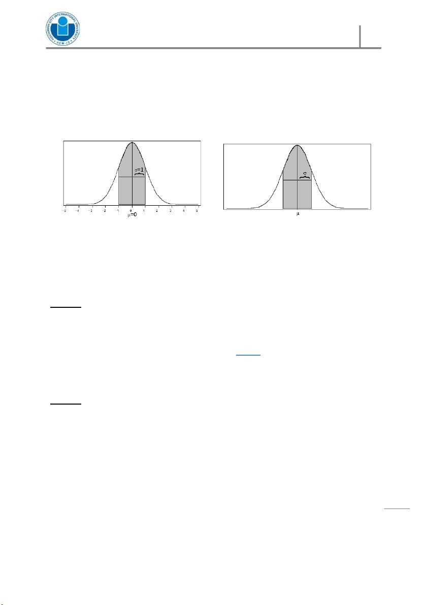
Sta ndard Normal Distribution Norma l Distribution
~
(
,
~
(
,
PART I
Finding probabilities of the normal distribution with given values
Step 01: Use the follow in g form ula t o t ransform t he norm al random variable ,
where ~
(
,
)
int o t he standard normal random variable , where
~
(
0, 1
)
.
=
Step 02: Use t he calculat or or Table 2 (Areas of St andard Normal Dist ribut ion) in
Appendix C t o com pute t he probabilities (or areas) of t he normal
distribut ion based on the standard nor mal distribut ion.
International University
IU
Powered by statisticsforbusinessiuba.blogspot.com
Stat ist ics for Business | Chapt er 04: The Norm al Distribut ion
2
CALCULATOR INSTRUCTION
Step No.01: Press M ODE 3: STAT [ AC ]
Step No.02: Press SHIFT + 1 | [ STAT ] 7: DISTR
After that, the calculator w ill show you 4 available symbols.
How ever, we just pay attention t o the first t hree ones.
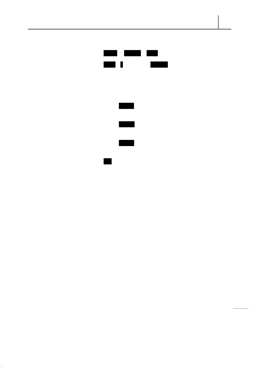
1 : P ( 2 : Q ( 3 : R (
+ We use t o compute the probability betw een the [ ]1 : P (
standard norm al random variable to , or −∞
(
<
)
+ We use [ 2 : Q ( ] t o comput e the probabilit y bet ween t he
standard norm al random variable to the mean or .
(
0 < <
)
+ We use [ 3 : R ( ] to compute the probab ility between t he
standard norm al random variable to . +
(
>
)
Step No.03: Press [ = ] t o get the result.
International University
IU
Powered by statisticsforbusinessiuba.blogspot.com
Stat ist ics for Business | Chapt er 04: The Norm al Distribut ion
3
Example | Part 1:
(Case of finding probabilities of the normal distribution with given values)
PROBLEM :
A psychologist has devised a st ress t est for dental pat ient s sit t ing in the w ait ing room s.
According t o this t est, t he stress scores (on a scale of 1 t o 10) for patients w aiting for root cana l
treatm ent s are found t o be approximately normally dist ributed w it h a m ean of 7.59 and a
st andard deviation of 0.73.
a. What percent age of such pat ients have a stress score low er than 6.0?
SOLUTION: = 7.59, = 0.73
Step 01:
(
< 6.0
)
= 󰇡

<
..
.
󰇢= (< 2.1781)
Step 02: M ODE 3 : STAT [ AC ]
SHIFT + 1| [STAT] 7 : DISTR 1 : P (-2.1781)
Then, press to get the result [ = ] −
(
.  
)
= .
Summ ing up,
(
< 6.0
)
= <( 2.1781) = 0.0147
b. What is t he probability t hat a randomly select ed root canal patient sit t ing in t he waiting
room has a stress score bet ween 7.0 and 8.0?
SOLUTION: = 7.59,= 0.73
Step 01:
(
7.0 < < 8.0
)
= 󰇡
..
.
<

<
..
.
󰇢
= 0.8082 < < 0.5616)
Step 02: (There are three different methods of using the pocket calculator
to solve the problem of calculating the probability betw een two
given values. You can use only one of three following methods
that depends on your choice, not all of them, since each of them
always provides the same result with others)
International University
IU
Powered by statisticsforbusinessiuba.blogspot.com
Stat ist ics for Business | Chapt er 04: The Norm al Distribut ion
4
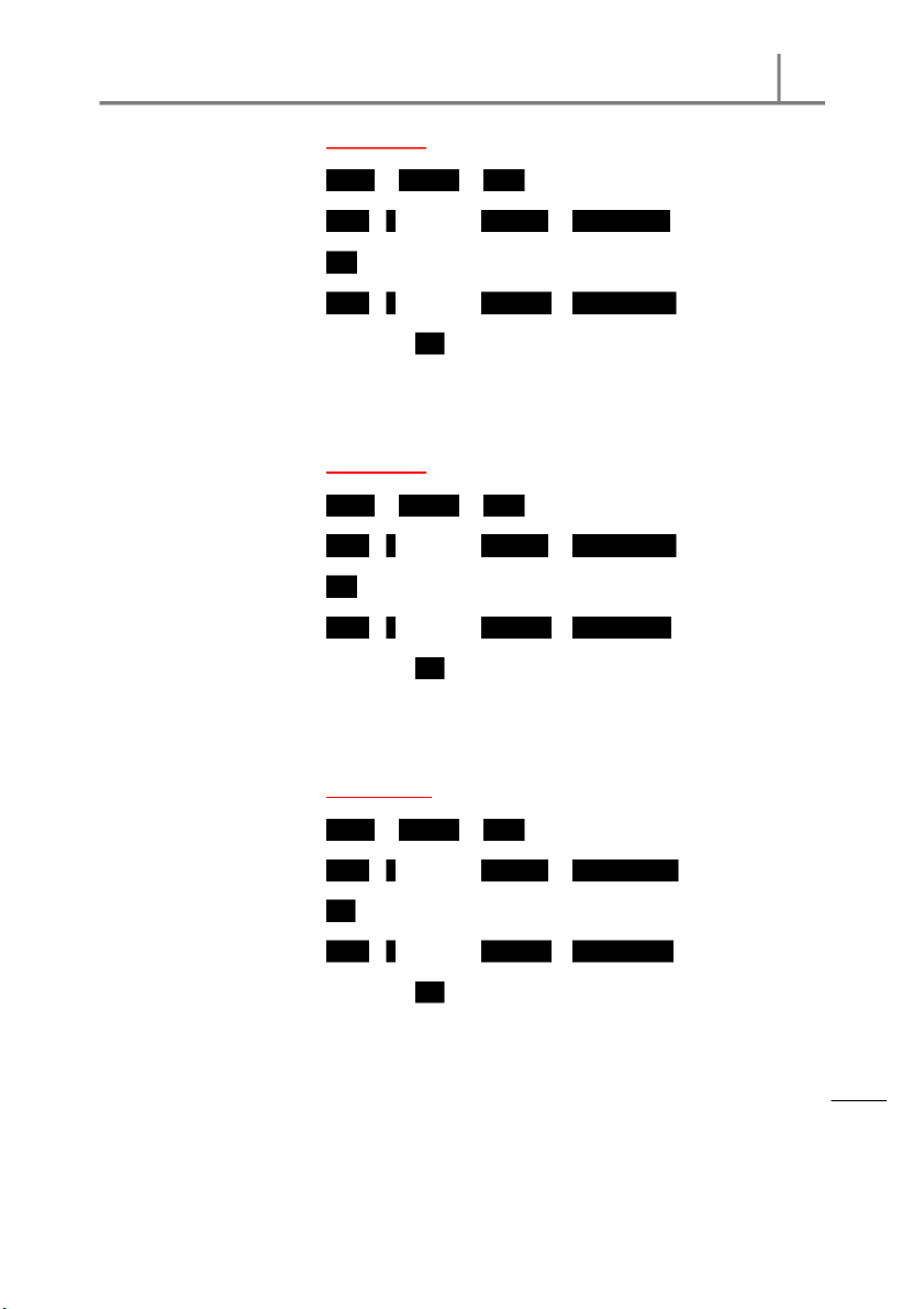
M ETHODS 01: Using 1 : P (
M ODE 3 : STAT [ AC ]
SHIFT + 1| [STAT] 7 : DISTR 1 : P (0.5616)
[ ]
SHIFT + 1| [STAT] 7 : DISTR 1 : P (-0.8082)
Then, press to get the result [ = ]
−
(
. 
) (
.  
)
= .
M ETHODS 02: Using 3 : R (
M ODE 3 : STAT [ AC ]
SHIFT + 1| [STAT] 7 : DISTR 3 : R (-0.8082)
[ ]
SHIFT + 1| [STAT] 7 : DISTR 3 : R (0.5616)
Then, press to get the result [ = ]
(
− .
) (
.
)
= .
M ETHODS 03: Using 2 : Q (
M ODE 3 : STAT [ AC ]
SHIFT + 1| [STAT] 7 : DISTR 2 : Q (-0.8082)
[ + ]
SHIFT + 1| [STAT] 7 : DISTR 2 : Q (0.5616)
Then, press to get the result [ = ]
(
−.
)
+
(
.
)
= . 
International University
IU
Powered by statisticsforbusinessiuba.blogspot.com
Stat ist ics for Business | Chapt er 04: The Norm al Distribut ion
5
Sum ming up,
(
7.0 < < 8.0
)
=
(
0.8082 < < 0.5616 = 0.5033
)
c. The psychologist suggest s t hat any patient w ith a st ress score of 9.0 or higher should be given
a sedative prior t o t reat ment. What percentage of pat ient s w ait ing for root canal t reatm ents
would need a sedative if this suggestion is accept ed?
SOLUTION: = 7.59,= 0.73
St ep 01:
(
9.0
)
= 󰇡

( ..
.
󰇢= (1.9315)
St ep 02: M ODE 3 : STAT [ AC ]
SHIFT + 1| [STAT] 7 : DISTR 3 : R (1.9315)
Then, press to get the result [ = ]
(
.
)
= . 
Summ ing up,
(
> 9.0
)
= (> 1.9315) = 0.0267
International University
IU
Powered by statisticsforbusinessiuba.blogspot.com
Stat ist ics for Business | Chapt er 04: The Norm al Distribut ion
6
PART II
Finding the values of X given a probability
Step 01: The probability t hat a norm al random variable w ill be above (below, or
symmetric) its m ean a certain number of st andard deviations is exactly
equal t o t he probability t hat the standard no rmal r andom variable w ill be
above (below , or symm etric) its mean the same number of (its) standard
deviations.
In particular,
(
>
)
=
(
>
)
(
<
)
=
(
<
)
−
(
< <
)
=
(
< <
)
Step 02: Find TA (Table Area)
(Table Area TA for a point of the st andard normal distribut ion is the area
given in the st andard normal probability t able o f Table 2 in Appendix C
under the standard normal cur ve betw een 0 and point > 0)
In particular,
For
(
>
)
:
If
(
>
)
< 0.5,  = .
(
>
)
If
(
>
)
> 0.5,  =
(
>
)
.
For
(
<
)
:
If
(
<
)
< 0.5,  = .
(
<
)
If
(
<
)
> 0.5,  =
(
<
)
.
For −
(
< <
)
,  −=
(
< <
)
/
International University
IU
Powered by statisticsforbusinessiuba.blogspot.com
Stat ist ics for Business | Chapt er 04: The Norm al Distribut ion
7
Step 03: Look inside Table 2 (Areas of the Standar d Normal Dist ribut ion) in
Appendix E for t he values of corresponding t o TA.
Step 04: Use the f ollow ing formula to transform the standard normal random
variable t o the normal random variable
= ± 
In par ticular,
For
(
>
)
:
If
(
>
)
< 0.5, t he value of will be posit ive , or +
If
(
>
)
> 0.5, t he value of will be negative, or −
For
(
<
)
:
If
(
<
)
< 0.5, t he value of will be negative, or −
If
(
<
)
> 0.5, t he value of will be positive, or +
For −
(
< <
)
, t he values of will include negative and positive
value, or and +
International University
IU
Powered by statisticsforbusinessiuba.blogspot.com
Stat ist ics for Business | Chapt er 04: The Norm al Distribut ion
8
Example | Part 2:
(Finding the values of X given a probability)
PROBLEM 01:
If X is a normally dist ributed random variable with mean 120 and st andard deviation 44, nd a
value x such that t he probability t hat X w ill be less than x is 0.56.
SOLUTION: We have ~
(
120,44
)
Step 01: W e are looking fo r t he value of the random variab le such t hat

(
<
)
= . . In order to f ind it , w e lo ok fo r the value of the
standard norm al deviation such t hat 
(
<
)
= . .
Step 02: If the area to the left of is equal to 0.56, the area bet ween 0 and (t he
Table Area) is equal to
 = . .= . .
Step 03: We look inside Table 2 (Areas of Standard Normal Distribution) in
Appendix C for the value corresponding to = 0.06 and find
= 0.15 = 0.0596 (actually,  , which is close enough to 0.06).
Step 04: We need t o find the appropriate value. Here we use t he following
equat ion.
= +   = +
(
.
) ( )
= .
International University
IU
Powered by statisticsforbusinessiuba.blogspot.com
Stat ist ics for Business | Chapt er 04: The Norm al Distribut ion
9
PROBLEM 02:
For a normal random variable with mean 19,500 and st andard deviation 400, a point of the find
distribution such that the probabilit y that t he random variable will exceed this value is 0.02.
SOLUTION: = 19,500, = 400
(
>
)
=
(
>
)
= 0.02
= 0.5 0.02 = 0.48
= 2.05
Thus, = + = 19,500 +
(
2.05
) (
400
)
= 20,320
PROBLEM 03
For , , symmetrically lying on each side of the mean,  ~ (32,7
) find two values
and
with
(
< <
)
= 0.99.
SOLUTION: = 32,= 7
(
< <
)
=
(
−< <
)
= 0.99
= 0.99/ 2 = 0.495
= 2.576
Thus,
= +
(
−
)
= 32 +
(
2.576
) (
7
)
= 13.968
= +
(
)
= 32 +
(
2.576
) (
7
)
= 50.032
International University
IU
Powered by statisticsforbusinessiuba.blogspot.com
Stat ist ics for Business | Chapt er 04: The Norm al Distribut ion
10
PART III
The Normal Approximation to the Binomial Distribution
When the number of t rials in a binomial distribut ion is large , t he calculat ion of ( > 100)
probabilit ies becom e difficult for t he pocket calculator. Fort unately, the binomial distribution as
increases and therefore w e can approxim at e it as normal dist ribut ion.
Condition:
Norma l Distribution as an Approxima tion t o Binomial Distribution
Usually, the normal dist ribut ion is used as an approximation t o the binom ial distr ibution
when  and are both greater than 5—that is, when ( 1 )
 > 5 and
( )
> 5
Step 1: Comput e and for the binomial distribut ion.
= 
= ( )
Step 2: Convert the discrete random var iable int o a cont inuous random variable.
Continuity Correct ion Factor
The addition of .5 and/ or subt ract ion of .5 from t he value(s) of when t he normal distribution
is used as an approximat ion to t he binomial dist ribut ion, where is t he num ber of successes in
t rials, is called t he cont inuit y cor rectio n factor.
Therefor e, when we calculat e the binomial probability of an int erval, we should subtra ct
0.5 from the left limit a nd a dd 0.5 t o t he right limit to get t he corresponding norm al
pr obability.
In par ticular,
 > , .
 < , .
 = , . .
International University
IU
Powered by statisticsforbusinessiuba.blogspot.com
Stat ist ics for Business | Chapt er 04: The Norm al Distribut ion
11
where = a no rmal variable w ith mean and st andard deviat ion
= a given value
Step 3: Comput e the required probabilit y using the normal distribut ion.
Example | Part 3:
(The Norm al Approximation to the Binomial Distribution)
PROBLEM :
CASIO Viet nam makes calculators. Consum er sat isfaction is one of the t op priorities of t he
com pany’s m anagement. The company guarant ees the refund of money or a replacement for
any calculator that m alfunct ions w it hin two years from the date of purchase. It is kn own from
past dat a t hat despite all ef fort s, 5% of the calculators manufact ured by this company
malfunction w ithin a 2-year period. The company recent ly mailed 500 such calculators t o its
cust omers.
a. Find t he probability t hat exactly 29 of t he 500 calculat ors w ill be returned for refund or
replacement w ithin a 2-year period.
SOLUTION:
Step 1: Compute and for the binomial distribution.
= = 500 × 0.05 = 25
=
( 1 ) = 500 × 0.05 × 0.95 =
95
2
4.8734
Step 2: Convert the discrete random variable into a continuous random variable.
To make the continuity cor rection, we subtract 0.5 from 29 and add 0.5 to 29, wh ich gives t he
int erval 28.5 t o 29.5 to obtain the value 29. Thus, for t he binomial problem will be ( = 29)
approximat ely equal t o (28.5 29.5) for the normal distribution.
Step 3: Compute the required probability using the normal distribution.
International University
IU
Powered by statisticsforbusinessiuba.blogspot.com
Stat ist ics for Business | Chapt er 04: The Norm al Distribut ion
12
(
28.5 29.5
)
=
28.5 25
95
2
29.5 25
95
2
󰇧
7
95
95
9
95
95
󰇨=
(
0.7182 0.9234
)
= 0.0584
Thus, based on the norm al approximation, t he probabilit y t hat exact ly 29 of the 500 calculators
will be ret urned for ref und or replacement w it hin a 2-year period is approximat ely 0.0584
b. What is t he probability t hat 27 or more of the 500 calculat ors will be returned for refund or
replacement w ithin a 2-year period?
SOLUTION:
Step 1: Compute and for the binomial distribution.
= = 500 × 0.05 = 25
=
( 1 ) = 500 × 0.05 × 0.95 =
95
2
4.8734
Step 2: Convert the discrete random variable into a continuous random variable.
For the cont inuity correct ion, w e subtract 0.5 from 27, w hich gives 26.5 to obt ain t he value 27.
Thus, for the bin omial pr oblem will be approximat ely equal to ( 27) ( 26.5) for the
norm al dist ribution.
Step 3: Compute the required probability using the normal distribution.
(
26.5
)
=
26.5 25
95
2
󰇧
3
95
95
󰇨=
(
0.3078
)
= 0.3791
Thus, based on the norm al approxim ation, the probability that 27 or more of the 500
calculat ors will be returned for ref und or replacement w ithin a 2-year period is approxim ately
0.3791
International University
IU
Powered by statisticsforbusinessiuba.blogspot.com
Stat ist ics for Business | Chapt er 04: The Norm al Distribut ion
13
c. What is the probability t hat 15 t o 22 of t he 500 calculat ors w ill be ret urned for refund or
replacement w ithin a 2-year period?
SOLUTION:
Step 1: Compute and for the binomial distribution.
= = 500 × 0.05 = 25
=
( 1 ) = 500 × 0.05 × 0.95 =
95
2
4.8734
Step 2: Convert the discrete random variable into a continuous random variable.
For t he continuit y correction, w e subt ract 0.5 f rom 15 and add 0.5 t o 22, which gives the
int erval 14.5 to 22.5 t o obt ain the int erval 15 t o 22. Thus, for the b inomial ( 15 22)
problem will be approximately equal to (14.5 22.5) for the normal dist ribution.
Step 3: Compute the required probability using the normal distribution.
(
14.5 22.5
)
=
14.5 25
95
2
22.5 25
95
2
󰇧−
21
95
95
95
91
󰇨=
(
2.1546 0.5130
)
= 0.2884
Thus, based on the normal approximat ion, the p robabilit y that 15 to 22 of t he 500 calculat ors
will be ret urned for ref und or replacement w it hin a 2-year period is approximat ely 0.2884
| 1/13

Preview text:

International University IU
STATISTICS FOR BUSINESS [IUBA] CHAPTER 04
THE NORM AL DISTRIBUTION
St a nda rd Norma l Distribut ion
Norma l Dist ribution
~ ( ,)
~ (,) PART I
Finding probabilities of the normal distribution with given values n tio u St ep 01:
Use t he follow in g form ula t o t r ansform t he norm al random var iable , trib
w here ~ (, ) int o t he standard normal random variable , where is l D ~ (0,1). a rm  −  o  = N e h : T 4 r 0 te St ep 02:
Use t he calculat or or Table 2 (Areas of St andard Norm al Dist ribut ion) in ap h
Appendix C t o com put e t he pr obab ilit ies (or ar eas) of t he norm al C
dist r ibu t ion based on t he st andar d nor m al dist ribut ion. s | es sin u r B s fo istic tat S
Powered by statisticsforbusinessiuba.blogspot.com 1
International University IU CALCULATOR INSTRUCTION
St ep No.01: Press M ODE3: STAT[ AC ]
St ep No.02: Press SHIFT + 1 | [ STAT ]7: DISTR
Aft er t hat , t he calculat or w ill show you 4 available sym bols.
How ever, w e just pay at t ent ion t o t he first t hree ones. 1 : P ( 2 : Q ( 3 : R (
+ We use [ 1 : P ( ] t o com put e t he pr obabilit y bet w een t he
st andard norm al random variable  to −∞, or (  < )
+ We use [ 2 : Q ( ] t o com put e t he probabilit y bet w een t he
st andard norm al random variable  to the mean or ( 0 <  < ) .
+ We use [ 3 : R ( ] t o com put e t he pr obab ilit y bet w een t he
st andard norm al random variable  to + ∞. (  > ) St ep No.03:
Press [ = ] t o get t he result . n tio u trib is l D a rm o N e h : T 4 r 0 te ap h C s | es sin u r B s fo istic tat S
Powered by statisticsforbusinessiuba.blogspot.com 2
International University IU Example | Part 1:
(Case of finding probabilities of the normal distribution with given values) PROBLEM :
A psychologist has devised a st ress t est for dent al pat ient s sit t ing in t he w ait ing room s.
According t o t his t est , t he st ress scores (on a scale of 1 t o 10) f or pat ient s w ait ing for root cana l
t reat m ent s are found t o be approximat ely norm ally dist ribut ed w it h a m ean of 7.59 and a
st andard deviat ion of 0.73.
a. W hat percent age of such pat ient s have a st ress score low er t han 6.0? SOLUTION:  = 7.59, = 0.73 .. St ep 01:
( < 6.0) =  󰇡 < 󰇢  = (  < −2.1781)  . St ep 02:
M ODE3 : STAT[ AC ]
SHIFT + 1| [STAT]
7 : DISTR1 : P (-2.1781) n tio
Then, press [ = ] t o get t he result ( −. ) = .  u trib
Sum m ing up, (  < 6.0) = (  < −2.1781) = 0.0147 is l D a
b. W hat is t he probabilit y t hat a random ly select ed root canal pat ient sit t ing in t he w ait ing rm
room has a st ress score bet w een 7.0 and 8.0? o N e SOLUTION: h  = 7.59, = 0.73 : T 4  .. St ep 01:
(7.0 <  < 8.0) =  󰇡.. < < 󰇢 r 0 .  . te ap
=  − 0.8082 <  < 0.5616) h C St ep 02:
(There are t hree different met hods of using t he pocket calculator s | es
to solve the problem of calculating the probability betw een tw o sin
given values. You can use only one of three follow ing methods u r B
that depends on your choice, not all of them, since each of them
alw ays provides the same result w ith others) s fo istic tat S
Powered by statisticsforbusinessiuba.blogspot.com 3
International University IU
M ETHODS 01: Using 1 : P (
M ODE3 : STAT[ AC ]
SHIFT + 1| [STAT]7 : DISTR1 : P (0.5616) [ ]
SHIFT + 1| [STAT]7 : DISTR1 : P (-0.8082)
Then, press [ = ] t o get t he result
(.) − (−.) = .
M ETHODS 02: Using 3 : R (
M ODE3 : STAT[ AC ]
SHIFT + 1| [STAT]7 : DISTR3 : R (-0.8082) [ ] n
SHIFT + 1| [STAT]7 : DISTR3 : R (0.5616) tio u
Then, press [ = ] t o get t he result trib is
(−.) − (.) = . l D a rm o N e
M ETHODS 03: Using 2 : Q ( h : T 4
M ODE3 : STAT[ AC ] r 0 te
SHIFT + 1| [STAT]7 : DISTR2 : Q (-0.8082) ap h C [ + ] s | es
SHIFT + 1| [STAT]7 : DISTR2 : Q (0.5616) sin u
Then, press [ = ] t o get t he result r B s fo
(−.) + (.) = . istic tat S
Powered by statisticsforbusinessiuba.blogspot.com 4
International University IU Sum m ing up,
(7.0 <  < 8.0) = (−0.8082 <  < 0.5616) = 0.5033
c. The psychologist suggest s t hat any pat ient w it h a st ress score of 9.0 or higher should be given
a sedat ive prior t o t reat m ent . W hat percent age of pat ient s w ait ing for root canal t reat m ent s
w ould need a sedat ive if t his suggest ion is accept ed? SOLUTION:  = 7.59, = 0.73 . St ep 01:
( ≥ 9.0) =  󰇡 ≥ (. 󰇢 = ( ≥ 1.9315)   . St ep 02:
M ODE3 : STAT[ AC ]
SHIFT + 1| [STAT]7 : DISTR3 : R (1.9315)
Then, press [ = ] t o get t he result ( .) = . 
Sum m ing up, (  > 9.0) = (  > 1.9315) = 0.0267 n tio u trib is l D a rm o N e h : T 4 r 0 te ap h C s | es sin u r B s fo istic tat S
Powered by statisticsforbusinessiuba.blogspot.com 5
International University IU PART II
Finding the values of X given a probability St ep 01:
The pro babilit y t hat a nor m al r ando m variable w ill be above (below , or
sym m et r ic) it s m ean a cert ain num ber of st andard deviat ions is exact ly
equal t o t he probabilit y t hat t he st andard no rm al r andom var iable w ill be
above (below , or sym m et r ic) it s m ean t he sam e num ber of (it s) st andar d deviat ions.
In part icular, ( > ) = ( > )
( < ) = ( < )
( <  < ) = (− <  < ) St ep 02: Find TA (Table Area)
(Table Ar ea TA f or a point  of t he standard normal distribut ion is t he area n
given in t he st andar d n orm al pr obabilit y t able o f Table 2 in Appendix C tio u
under t he st andar d nor mal cur ve bet w een 0 and point  > 0) trib is In part icular, l D a For rm ( > ): o N e
If ( > ) < 0.5,  = .  − ( > ) h : T 4
If ( > ) > 0.5,  = ( > ) − .  r 0 te For ( < ) : ap h C
If ( < ) < 0.5,  = .  − ( < ) s | es
If ( < ) > 0.5,  = ( < ) − .  sin u r B
For (− <  < ) ,  = ( − <  < )/  s fo istic tat S
Powered by statisticsforbusinessiuba.blogspot.com 6
International University IU St ep 03:
Look inside Table 2 (Areas of t he St andar d Norm al Dist r ibut ion) in
Appendix E for t he values of  corresponding t o TA. St ep 04:
Use t he f ollow ing form ula t o t r ansf or m t he st andard norm al ran dom
var iable  to t he normal random variable   =  ±  In par t icular , For ( > ) :
If ( > ) < 0.5, t he value of “ ” will be positive, or + 
If ( > ) > 0.5, the value of “ ” will be negative, or − For ( < ) :
If ( < ) < 0.5, the value of “ ” will be negative, or − n
If ( < ) > 0.5, the value of “ ” will be positive, or +  tio u
For (− <  < ) , t he values of “ ” will include negative and positive trib is
value, or –  and +  l D a rm o N e h : T 4 r 0 te ap h C s | es sin u r B s fo istic tat S
Powered by statisticsforbusinessiuba.blogspot.com 7
International University IU Example | Part 2:
(Finding the values of X given a probability) PROBLEM 01:
If X is a norm ally dist ribut ed random variable w it h m ean 120 and st andard deviat ion 44, find a
value x such t hat t he probabilit y t hat X w ill be less t han x is 0.56.
SOLUTION: We have ~ ( 120,44) St ep 01:
W e are looking fo r t he value of t he random var iab le  such that
( < ) = .. In order to find it, we look for the value of the
st andard norm al deviat ion  such that (  < ) = . . St ep 02:
If t he area t o t he left of  is equal to 0.56, the area between 0 and  (the Table Area) is equal t o n
 = . − . = .. tio u trib is St ep 03:
We lo ok inside Table 2 (Areas of St andard Norm al Dist ribut ion) in l D a
Appendix C for t he  value corresponding to  = 0.06 and find rm
 = 0.15 (actually,  = 0.0596, which is close enough to 0.06). o N e h : T 4 St ep 04:
We need t o find t he appr opr iat e  value. Here we use the following r 0 equat ion. te ap h
 =  +  =  + (.)() = . C s | es sin u r B s fo istic tat S
Powered by statisticsforbusinessiuba.blogspot.com 8
International University IU PROBLEM 02:
For a norm al random variable w it h mean 19,500 and st andard deviat ion 400, find a point of t he
dist ribut ion such t hat t he probabilit y t hat t he random variable w ill exceed t his value is 0.02.
SOLUTION:  = 19,500, = 400
( > ) = ( > ) = 0.02  = 0.5 − 0.02 = 0.48  = 2.05
Thus,  =  +  = 19,500 + ( 2.05) (400) = 20,320 PROBLEM 03
For ~ ( 32,7) , find two values 
, sym met rically lying on each side of t he m ean, and 
w it h (  <  < ) = 0.99. SOLUTION:  = 32, = 7 n tio
( <  < ) = (− <  < ) = 0.99 u trib  = 0.99/ 2 = 0.495 is l D  = 2.576 a rm Thus, o
 =  + (−) = 32 + (−2.576)(7) = 13.968 N e h
 =  + () = 32 + (2.576)(7) = 50.032 : T 4 r 0 te ap h C s | es sin u r B s fo istic tat S
Powered by statisticsforbusinessiuba.blogspot.com 9
International University IU PART III
The Normal Approximation to the Binomial Distribution
When t he num ber of t rials  in a binomial distribution is large ( > 100), t he calculat ion of
probabilit ies becom e dif ficult for t he pocket calculat or. Fort unat ely, t he binom ial dist ribut ion as
 increases and therefore we can approximate it as normal distribution. Condit ion:
Norma l Dist ribution as an Approxima t ion t o Binomial Dist ribut ion
Usually, t he norm al dist r ibut ion is used as an approxim at ion t o t he binom ial dist r ibut ion
w hen  and ( 1 − ) are bot h greater than 5—that is, w hen
 > 5 and( − ) > 5
St ep 1: Com put e  and  for the binomial distribut ion. n  = 
 = ( − ) tio u
St ep 2: Conver t t he discr et e random var iable int o a cont inu ous rand om var iab le. trib is
Cont inuit y Correct ion Fa ct or l D a
The addit ion of .5 and/ or subt ract ion of .5 from t he value(s) of  when t he normal distribution rm o
is used as an approxim at ion t o t he bin om ial dist ribut ion , w here  is the number of successes in N e h
 trials, is called the continuity correction factor. : T 4
Ther efor e, w hen w e calculat e t he binom ial probabilit y of an int er val, w e should subt ra ct r 0 te
0.5 from t he left limit a nd a dd 0.5 t o t he right limit t o get t he corr esponding nor m al ap h pr obabilit y. C s | In par t icular , es sin u
 > ,. r B
 < ,. s fo istic
 = ,.. tat S
Powered by statisticsforbusinessiuba.blogspot.com 10
International University IU
w here  = a normal variable with mean  and st andard deviat ion   = a given value
St ep 3: Com put e t he required pr obabilit y using t he nor m al dist r ibut ion. Example | Part 3:
(The Normal Approximation to the Binomial Distribution) PROBLEM :
CASIO Viet nam m akes calculat ors. Consum er sat isf act ion is one of t he t op priorit ies of t he
com pany’s m anagem ent . The com pany guarant ees t he refund of m oney or a replacement for
any calculat or t hat m alfunct ions w it hin t w o years from t he dat e of purchase. It is kn own from
past dat a t hat despit e all ef fort s, 5% of t he calculat ors m anufact ured by t his company n
m alfunct ion w it hin a 2-year period. The company recent ly m ailed 500 such calculat ors t o it s tio u cust om ers. trib is
a. Find t he probabilit y t hat exact ly 29 of t he 500 calculat ors w ill be ret urned for refund or l D
replacem ent w it hin a 2-year period. a rm o SOLUTION: N e h
Step 1: Compute and for the binomial distribution. : T 4
 =  = 500 × 0.05 = 25 r 0 te ap √95 h
 = (1 − ) = √500 × 0.05 × 0.95 = ≈ 4.8734 C 2 s |
Step 2: Convert the discrete random variable int o a continuous random variable. es sin u
To m ake t he cont inuit y cor rect ion, w e subt ract 0.5 from 29 and add 0.5 t o 29, w h ich gives t he r B
int erval 28.5 t o 29.5 t o obt ain t he value 29. Thus, (  = 29) for the binomial problem will be s fo
approximat ely equal t o ( 28.5 ≤  ≤ 29.5) for the normal distribution. istic
Step 3: Compute the required probability using the normal distribution. tat S
Powered by statisticsforbusinessiuba.blogspot.com 11
International University IU  − 
(28.5 ≤  ≤ 29.5) =  28.5 − 25 ≤  √95  ≤ 29.5 − 25 √95 2 2
 󰇧7√95 ≤  ≤ 9√95󰇨 = (0.7182 ≤  ≤ 0.9234) = 0.0584 95 95
Thus, based on t he norm al approxim at ion, t he pr obabilit y t hat exact ly 29 of t he 500 calculat ors
w ill be ret urned for ref und or replacem ent w it hin a 2-year period is approxim at ely 0.0584
b. W hat is t he probabilit y t hat 27 or more of t he 500 calculat ors w ill be ret urned for refund or
replacem ent w it hin a 2-year period? SOLUTION:
Step 1: Compute and for the binomial distribution.
 =  = 500 × 0.05 = 25 √95 n
 = (1 − ) = √500 × 0.05 × 0.95 = ≈ 4.8734 2 tio u
Step 2: Convert the discrete random variable int o a continuous ra ndom variable. trib is
For t he cont inu it y correct ion, w e subt ract 0.5 fr om 27, w hich gives 26.5 t o obt ain t he value 27. l D a
Thus, (  ≥ 27) for the binomial problem will be approximately equal to (  ≥ 26.5) for the rm o norm al dist r ibut ion. N e h
Step 3: Compute the required probability using the normal distribution. : T 4 r 0  −  te ( ≥ 26.5) =    ap  ≥ 26.5 − 25 √95 h C 2 s | es
 󰇧 ≥ 3√95󰇨 = ( ≥ 0.3078) = 0.3791 sin 95 u r B
Thus, based on t he norm al approxim at ion, t he probabilit y t hat 27 o r m ore of t he 500 s fo
calculat ors w ill be ret urned f or ref und or replacem ent w it hin a 2-year per iod is appr oxim at ely istic 0.3791 tat S
Powered by statisticsforbusinessiuba.blogspot.com 12
International University IU
c. W hat is t he probabilit y t hat 15 t o 22 of t he 500 calculat ors w ill be ret urned for refund or
replacem ent w it hin a 2-year period? SOLUTION:
Step 1: Compute and for the binomial distribution.
 =  = 500 × 0.05 = 25  √95
= ( 1 − ) = √500 × 0.05 × 0.95 = ≈ 4.8734 2
Step 2: Convert the discrete random variable int o a continuous ra ndom variable.
For t he cont inuit y cor rect ion, w e subt ract 0.5 f rom 15 and add 0.5 t o 22, w hich gives t he
int erval 14.5 t o 22.5 t o obt ain t he int erval 15 t o 22. Thus, ( 15 ≤  ≤ 22) for the binom ial
problem w ill be approxim at ely equal t o (14.5 ≤  ≤ 22.5) for the normal distribution.
Step 3: Compute the required probability using the normal distribution.  − 
(14.5 ≤  ≤ 22.5) =  14.5 − 25 ≤  √95  ≤ 22.5 − 25 √95 n 2 2 tio u √95 trib
 󰇧− 21√95 ≤  ≤ −
󰇨 = (−2.1546 ≤  ≤ −0.5130) = 0.2884 is 95 91 l D a
Thus, based on t he no rm al approxim at ion, t he p robabilit y t hat 15 t o 22 of t he 500 calculat ors rm o
w ill be ret urned for ref und or replacem ent w it hin a 2-year period is approxim at ely 0.2884 N e h : T 4 r 0 te ap h C s | es sin u r B s fo istic tat S
Powered by statisticsforbusinessiuba.blogspot.com 13