Chapter 11 - Multiple Regression - Statistics for Business | Trường Đại học Quốc tế, Đại học Quốc gia Thành phố HCM
Chapter 11 - Multiple Regression - Statistics for Business | Trường Đại học Quốc tế, Đại học Quốc gia Thành phố HCM được sưu tầm và soạn thảo dưới dạng file PDF để gửi tới các bạn sinh viên cùng tham khảo, ôn tập đầy đủ kiến thức, chuẩn bị cho các buổi học thật tốt. Mời bạn đọc đón xem!
Môn: Statistics for Business (BAO8OIU) 43 tài liệu
Trường: Trường Đại học Quốc tế, Đại học Quốc gia Thành phố Hồ Chí Minh 1.9 K tài liệu
Tác giả:


Preview text:
International University IU
STATISTICS FOR BUSINESS [IUBA] CHAPTER 11 M ULTIPLE REGRESSION STRUCTURE OF PAPER
PART I - M ULTIPLE REGRESSION M ODEL
PART II - M EASURES OF PERFORM ANCE OF A REGRESSION M ODEL AND THE ANOVA TABLE
PART III - THE F – TEST OF A M ULTIPLE REGRESSION M ODEL
PART IV - TESTS OF THE SIGNIFICANCE OF INDIVIDUAL REGRESSION PARAM ETERS n io s s re g e R le ltip u : M 1 r 1 te ap h C s | es sin u r B s fo istic tat S
Powered by statisticsforbusinessiuba.blogspot.com 1
International University IU PART I
M ULTIPLE REGRESSION M ODEL
The populat ion r egression m odel of a dependent variable on a set of independent
var iables ,,… , is given by
= + + + ⋯ + +
w here is t he intercept of the regression surface and each , = 1,… , is the slope
of t he regression sur face – som et im es called t he response sur face – w it h respect t o var iable . M odel Assum ptions:
1. For each observat ion , t he er ror t erm is normally distribut ed wit h mean zero and standard
deviat ion and is independent of the error terms associated wit h all ot her observations. That is,
~ (0,) for all = 1,2,…, independent of ot her errors. n
2. In t he cont ext of regression analysis, t he var iables io
are considered fix quantit ies, although s s
in t he cont ext of correlat ional analysis, t hey are random variab les. In any case, re g
ℎ . When we assume that are fixed quantities, we are e R
assum ing t hat w e have realizat ion of varibles and that the only randomness in comes le from t he error t erm . ltip u : M 1 r 1
The Est imat ed Regression Relat ionship te ap
The est im at ed regression relat ionship is h C s |
= + + + ⋯ + es sin u
w here is t he predicted value of , the value lying on t he estimated regression surface. r B
The t erm s , = 0,…,, are the least-squares estimates of the population regression s fo par am et er s . istic tat S
Powered by statisticsforbusinessiuba.blogspot.com 2
International University IU PART II
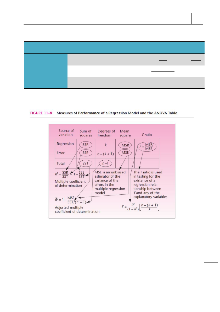
M EASURES OF PERFORM AM CE OF A REGRESSION M ODEL AND THE ANOVA TABLE
M ean Square Error ( )
St andard Error of Estimate ( )
and are measures of how well the regression fits the data = − = √ ( + )
M ultiple Correlation Coefficient ( )
M ult iple Coefficient of Det erm inat ion ( )
Adjusted M ult iple Coefficient of Det erm inat ion ( )
, , and are measures of how well the regression model fits the data. In other n
w ords, t hey m easure t he per cent age of var iat ion in t he dependent var iable explained io s
by t he indepen dent var iables s re g e
M ult iple Correlat ion Coefficient R le ltip = u : M
M ult iple Coefficient of Determination 1 r 1 te = ap h
= − C s |
Adjusted M ult iple Coefficient of Determination es sin
/ [ − ( + )] − u = − = − ( − ) r B / ( − ) − ( + ) s fo istic tat S
Powered by statisticsforbusinessiuba.blogspot.com 3
International University IU
ANOVA Table for M ultiple Regression M odel Sum of Squares M ean Square F. ratio Source of Variat ion ( ) ( ) () Regression = () = Error − ( + 1) = ( ) − ( + 1) Tot al − 1 ( ) n io s s re g e R le ltip u : M 1 r 1 te ap h C s | es sin u r B s fo istic tat S
Powered by statisticsforbusinessiuba.blogspot.com 4
International University IU PART III
THE F – TEST OF A M ULTIPLE REGRESSION M ODEL
F – test of a mult iple regression model is a st at ist ical hypot hesis test for the existence
of a linear relat ionship bet ween and any of the
F – test of a M ultiple Regression M odel
HYPOTHESIS TESTING PROCESS: STEP 01:
Det er mine t he nu ll and alt ernat io n hypot hesis:
= = = = ⋯ = =
= ( = ,…,) STEP 02:
Const r uct t he ANOVA Table f or t he m ult iple regression m odel n Sum of Squares M ean Square F. ratio io s Source of Variat ion s ( ) ( ) () re g Regression e = R () = le Error ltip − ( + 1) = ( u ) − ( + 1) Tot al : M − 1 1 ( ) r 1 te ap h STEP 03:
Com put e t he t est st at ist ic value ( C
) (based on the ANOVA table) and t he s |
cr it ical value ( ) (based on the level of significance) es sin The t est st at ist ic value: u r B s fo
= − = istic tat S
Powered by statisticsforbusinessiuba.blogspot.com 5
International University IU
At t he level of significance, t he cr it ical value:
= ,,() STEP 04: CONCLUSION
+ Sit uat ion 01: We cannot reject t he null hypo t hesis since <
For t he inst ance t hat t he null hypo t hesis is t r ue, no linear r elat ionship
exist s bet w een t he dependent var iable and any of t he independent
var iables in the proposed regression model.
+ Sit uat ion 02: We can reject t he null hypot hesis since >
For t he inst ance t hat w e can reject t he null hypot hesis, t her e is
st at ist ical evidence t o conclude t hat a regr ession r elat ion ship exist s
bet w een t he dependent var iable and at least one of the independent
var iables proposed in the regression model. n io s s re g e R le ltip u : M 1 r 1 te ap h C s | es sin u r B s fo istic tat S
Powered by statisticsforbusinessiuba.blogspot.com 6
International University IU PART IV
TESTS OF THE SIGNIFICANCE OF INDIVIDUAL REGRESSION PARAM ETERS
A test for t he significance of an individual parameters is important because it tells us
not only whether there is evidence that variable ( = 1, …, ) has a linear
relationship w it h Y but also whet her there is st at istical evidence t hat variable has
explanat ory power wit h respect to the dependent variable .
Tests of the Significance of Individual Regression Paramet ers
HYPOTHESIS TESTING PROCESS: STEP 01:
Det er mine t he nu ll and alt ernat ive hypo t heses:
(Not e: They a re t w o t ailed-test ing) (1) : = 0 : ≠ 0 n (2) io : = 0 s s : ≠ 0 re g e R … … le ltip (k) u : = 0 : ≠ 0 : M 1 r 1 te ap h C s | es sin u r B s fo istic tat S
Powered by statisticsforbusinessiuba.blogspot.com 7
International University IU STEP 02:
Com put e t he t est st at ist ic value ( / ) and the critical values ( / )
based on t he level of signif icance
+ Sit uation 01: If − ( + 1) < 30, w e use −
For t est ( = 1, …, ), t he test st atistic value: − = ( )
At t he level of significance ( ) , the critical values: ± = ± ,()
+ Sit uation 02: If − ( + 1) ≥ 30, w e use −
For t est ( = 1, …, ), t he test st atistic value: − n = io ( s ) s re g
At t he level of significance ( ) , the critical values: e R le ± = ± ltip u : M 1 r 1 te ap h C s | es sin u r B s fo istic tat S
Powered by statisticsforbusinessiuba.blogspot.com 8
International University IU STEP 03: CONCLUSION
At t he level of significance, for each t est ,
+ Sit uat ion 01: We cannot reject since ∈ [−,] or ∈ [−,]
For t he inst ance t hat t he null hypot hesis is t r ue t hat t he slope
par am et er of is non – significant and no linear relationship exists
bet w een t he dependent var iable and the independent variable
+ Sit uat ion 02: We can reject since ∉ [−, ] or ∉ [−,]
For t he inst ance t hat w e can r eject t he nu ll h ypot hesis, t he var iable
is significant . It m eans t hat t her e is st at ist ical evidence t hat variable
has a linear r elat ionship w it h and explanat ory pow er wit h respect t o t he dependent var iable. n io s s re g e R le ltip u : M 1 r 1 te ap h C s | es sin u r B s fo istic tat S
Powered by statisticsforbusinessiuba.blogspot.com 9
International University IU
Example: (Case of M ultiple Regression Analysis)
PROBLEM 01: (The Form of M ultiple-Choice Questions)
The sam ple dat a size 12 t aken fr om f our populat ions. The SPSS out p ut for regression
analysis is as f ollow s w h ich ar e m issin g som e values: n = 12, k = 4 − 1 = 3 ANOVA M odel Sum of Squares Df M ean Square F Sig. 1 Regression 80.117 3 26.706 56.700 0.000 Residual 3.768 8 0.471 Tot al 83.885 11
a Predict or s: (Co nst ant ), X1, X2, X3 b Dependent Variable: Y Coefficient s n M odel Coefficient s Std. Error t Sig. io s s 1 (Const ant ) 45.56 5.674 re g X1 2.754 0.775 3.5535 0.0075 e R X2 3.56 1.107 3.2159 0.0123 le X3 1.85 1.065 1.7371 0.1206 ltip u Depen dent Var iable: Y = 0.05 : M 1
1. Fill in the ANOVA table and coefficients table by the relevant values at the suit cell. r 1 te ap h C s | es sin u r B s fo istic tat S
Powered by statisticsforbusinessiuba.blogspot.com 10
International University IU
2. Comment on t he result of Regression: SOLUSION
: = = = 0
: ℎ ( = 1,2,3)
Since t he t est st at ist ic value is t o o large ( F = 56.7), we can strongly reject H at all
level of signif icance. It m eans t hat based on t he ANOVA t able for regression m odel
and t he hypot hesis t est ing, w e have enough evidence t o pr ove t hat t her e is a
regression r elat ionship bet w een t he depen dent var iable Y and t he indepen dent var iables Xi.
3. Using = 0.05, X3 is a significant predictor : (1 point ) a. True b. False SOLUTION : 3b. False H n : β = 0 io s s H: β ≠ 0 re g e
Based on t he t able of coef ficient s, t he p-value is lar ge, t hat is, t he t est st at ist ic value R le
falls in t he no n-r eject ion region. So, w e canno t reject H at 0.05 level of significance. ltip u
It m eans t hat based on t he t able and t he hypot hesis t est ing, w e can believe t hat t he : M
var iable X3 is not signif icant predict or . 1 r 1 te ap h C s | es sin u r B s fo istic tat S
Powered by statisticsforbusinessiuba.blogspot.com 11
International University IU
4. What is this model predict with X1=10, X2=15, X3=50? a. 160 b. 219 c. 238
d. Other …………………………………………… SOLUTION : 4b. 219
Based on t he t able o f coeff icient s, w e can est im at e t he m ult iple regression m odel f or pr edict or as fo llow ings: Y
= 45.560 + 2.754X + 3.56X + 1.85X Y
= 45.560 + 2.754 × 10 + 3.56 × 15 + 1.85 × 15 = 219
5. Compute the value of R: 97.700% SOLUTION
R = SSR = 80.117 = 0.977 = 97.700% n SST 83.885 io s s re g e R le ltip u : M 1 r 1 te ap h C s | es sin u r B s fo istic tat S
Powered by statisticsforbusinessiuba.blogspot.com 12
International University IU
PROBLEM 02: (The Form of W riting Questions)
A gr ocery st ore forecast s t he m ont hly demand (Y) for t heir pr oduct s using m ult iple-
regr ession. Thr ee independent var iables used ar e X1, X2, and X3. The dat a for last 12 mont hs
of t he year 2010 are collect ed. The regression result s are show n below : ANOVA table: Source SS df M S F Regression Residual Err or Tot al 625.667 Coefficient s Predict ors Coefficient s S.E. of coefficient s t Const ant -29.743 12.903 X1 1.104 0.283 X2 1.106 0.205 X3 -0.169 0.198 n io s
R2 = 94.76%. Level of significance is α = 0.05. s re g e R le
1. Fill up the ANOVA table; give the comment s on relationships among variables. ltip u SOLUTION : M 1 r 1 Source SS df M S F te Regression 593.132 3 197.711 48.615 ap h Residual Err or 32.535 8 4.067 C Tot al 625.667 11 s | es sin u R = 1 or SSE = SST( 1 r B −
− R) = 625.667(1 − 0.948) = 32.535 s fo istic tat S
Powered by statisticsforbusinessiuba.blogspot.com 13
International University IU
: = = = 0
: ℎ ( = 1,2,3)
Since t he t est st at ist ic value is t o o lar ge ( F = 48.615), we can strongly reject H at
all level of signif icance. It m eans t hat based on t he ANOVA t ab le for regression
m odel an d t he hypot hesis t est ing, w e have enough evidence t o pr ove t hat t here is a
regression relat ionship bet w een t he dependent variable Y and the independent var iables X (i = 1,2,3) .
2. Write the regression equation. What predict or should be removed from the equation? SOLUTION Predict ors Coefficient s S.E. of coefficient s t Const ant -29.743 12.903 X1 1.104 0.283 3.901 X2 1.106 0.205 5.395 X3 -0.169 0.198 0.854 n io
From t he t ab le, w e can set up t he regression equat ion as f ollow in gs: s s re g Y = e
−29.743 + 1.104X + 1.106X − 0.169X + ε R le ltip u
To t est w het her t he var iables of t he regressio n m odal are signif icant , w e have t o : M 1
conduct t he t -t est of individual regressio n par am et ers. r 1 te
Our nu ll and alt ernat ive hypot hesizes of each variable: ap h C H : β = 0 H : β = 0 H: β = 0 s | H : β ≠ 0 H : β ≠ 0 H: β ≠ 0 es sin u r B s fo istic tat S
Powered by statisticsforbusinessiuba.blogspot.com 14
International University IU
Based on t he t able o f coeff icient s, w e can com put e t he t est st at ist ic value of each var iable as fo llow ings: b − 0 1.104 t = = 3.901 = s( b) 0.283 b − 0 1.106 t = = = 5.395 s( b) 0.205 b − 0 −0.169 t = = = −0.854 s( b) 0.198 df = n − (k + 1) = 8
α = 0.05,/ 2 = 0.05/ 2 = 0.025
The crit ical value: ± t = ± t,/ = ± t,. = ± 2.306
Thus, at 0.05 level of signif icance, f or t he inst ance of X and X, we can reject H. n
On t he ot her hand, w e cannot r eject t he null hypot hesis of X since t belong t o io s s
t he non-r eject ion r egion. It m eans t hat based on t he hypot hesis t est ing, w e have re g
enough evidence t o prove t hat t he var iables X X e
and X are significant. However, R
is not signif icant and should be rem oved fr om t he r egression equat ion. An d w e le
should conduct t he mu lt iple regression m odel again. ltip u : M 1 r 1 te ap h C s | es sin u r B s fo istic tat S
Powered by statisticsforbusinessiuba.blogspot.com 15
Tài liệu liên quan:
-
Đề thi giữa kỳ học phần Statistics for Business năm 2015 | Trường Đại học Quốc tế, Đại học Quốc gia Thành phố Hồ Chí Minh
323 162 -
Đề thi giữa kỳ học phần Statistics for Business có đáp án | Trường Đại học Quốc tế, Đại học Quốc gia Thành phố Hồ Chí Minh
385 193 -
Đề thi giữa kỳ học phần Statistics for Business năm 2019 | Trường Đại học Quốc tế, Đại học Quốc gia Thành phố Hồ Chí Minh
270 135 -
Đề thi giữa kỳ học phần Statistics for Business | Trường Đại học Quốc tế, Đại học Quốc gia Thành phố Hồ Chí Minh
283 142 -
Bài tập tiểu luận nhóm học phần Statistics for Business | Trường Đại học Quốc tế, Đại học Quốc gia Thành phố Hồ Chí Minh
293 147