Chapter 14 - Square Testing - Statistics for Business | Trường Đại học Quốc tế, Đại học Quốc gia Thành phố HCM

International University IU
STATISTICS FOR BUSINESS [IUBA] CHAPTER 14 CHI - SQUARE TESTING
CHI – SQUARE TESTING PROCESS STEP 01:
Det er mine t he nu ll and alt ernat ive hypo t heses STEP 02:
Det er mine t he expect ed coun t s and obser ved count s of dat a point s in dif fer ent cells. STEP 03:
Com put e t he t est st at ist ic value (based o n t he dif ference bet w een t he
obser ved and t he expect ed ; Hint : Est ab lishin g a t able) and t he cr it ical value
(based on t he level of signif icance and chi – squar e dist r ibut ion). STEP 04:
Com pare t he t est st at ist ic value w it h t he cr it ical value and m ake a decision. sts e T re a u q i - S h : C 4 r 1 te ap h C ss | e sin u r B s fo istic tat S
Pow ered by statisticsforbusinessiuba.blogspot.com 1
International University IU PART I
A CHI – SQUARE TEST FOR GOODNESS OF FIT
CHI-SQUARE TESTING PROCESS STEP 01:
Det er mine t he nu ll and alt ernat ive hypo t heses
: The probabilities of occurrence of events , ,…, are given by
t he specif ied pr obabilit ies ,,…,
: The probabilities of the  events not the  stated in the null hypot hesis STEP 02:
Det er mine t he observed count s and t he expect ed count s (  = ) of data point s in dif ferent cells. STEP 03:
Com put e t he t est st at ist ic value and t he crit ical value
The t est st at ist ic value (based o n t he dif fer ence bet w een t he obser ved and t he expect ed): sts  e (  T   − )   =  re  a  u  q
Hint : Est ablishing a t able i - S h : C
The cr it ical value (based on t he level of significance ( 4 )): r 1   te
 = , ap h C STEP 04:
Com pare t he t est st at ist ic value w it h t he cr it ical value and m ake a decision. ss | e
Based on t he level of signif icance, sin u
+ W e can reject t he null hypot hesis   >  r B  if   s fo
+ W e cannot reject t he null hypot hesis   
 if  <  istic tat S
Pow ered by statisticsforbusinessiuba.blogspot.com 2
International University IU
Example 14.01: Case of Chi – Square Testing for Goodness of Fit PROBLEM
In a biology laborat ory t he m at ing of t w o red -eyed fruit flies yielded  = 576 offspring, among
w hich 338 w ere red-eyed, 102 w ere brow n-eyed, 112 w ere scarlet -eyed, and 24 w ere w hit e-eyed.
Use t hese dat a t o t est , w it h  = 0.05, the hypot hesis t hat the rat io among the offspring w ould be
9: 3: 3: 1, respect ively. SOLUTION
 = 4,  = k − 1 = 4 − 1 = 3 Let
( ) be the event that off-springs are red-eyed.
( ) be the event that off-springs are brown-eyed.
( ) be the event that off-springs are scarlet-eyed.
( ) be the event that off-springs are white-eyed.
: The four off-springs are equally preferred; that is, the probabilities of choosing any of the off- springs are equal 9: 3: 3: 1 
: Not all four off-springs are equally preferred; t hat is, the probabilities of choosing any of the
off -spr ings are not equal 9: 3: 3: 1 sts e T 9 3 3 1 re a 9: 3: 3: 1 = : : : u 16 16 16 16 q i - S 9 3 h  =  = 576 × = 324  = 108 16  =  = 576 × 16 : C 4  3 1  =  = 576 × = 108  =  = 576 × = 36 r 1 16 16 te ap h C
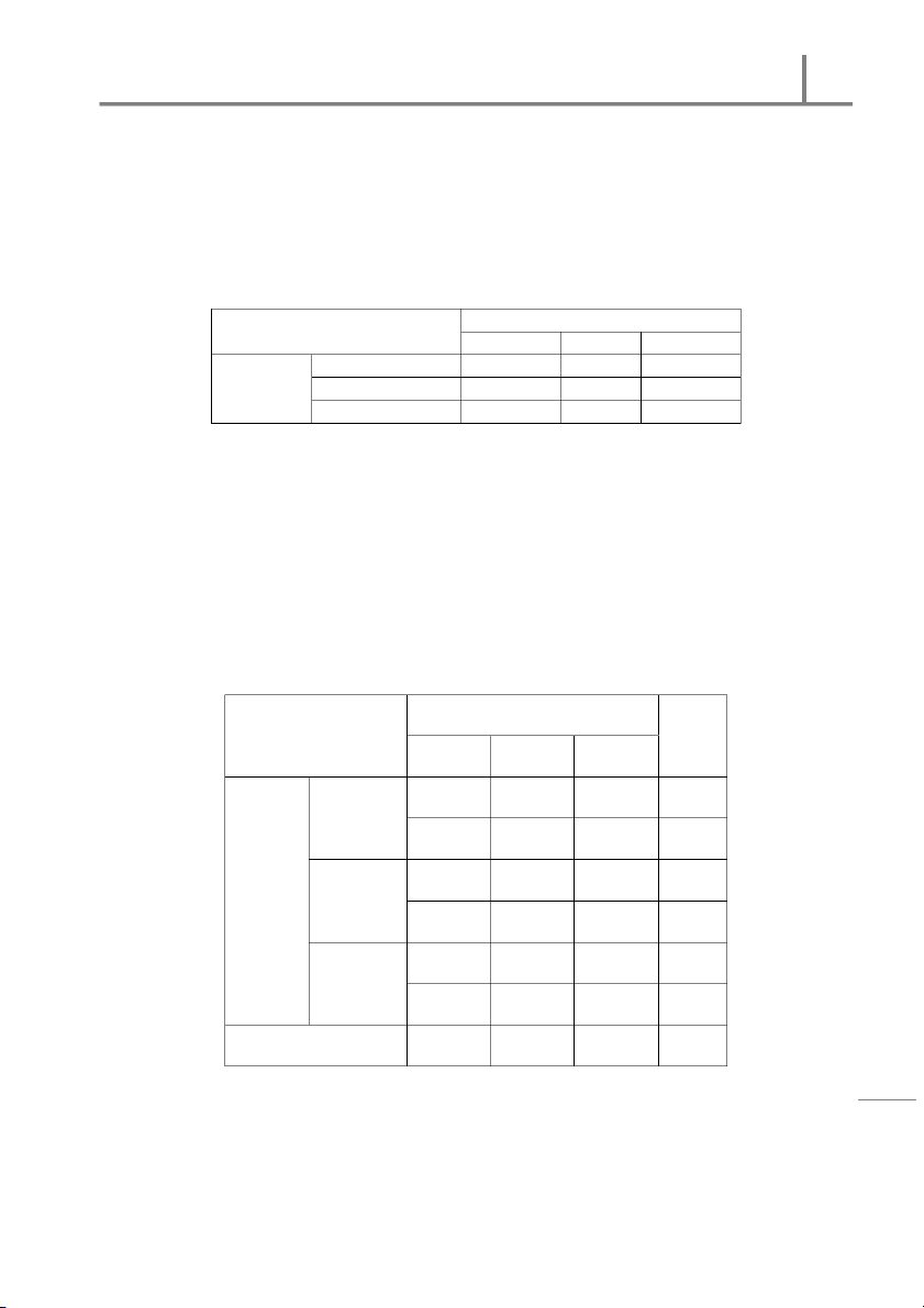
TABLE: Observed Count s (w it h t he expect ed count s show n in parent heses) ss | e Red-eyed Brow n-eyed Scarlet -eyed Whit e-eyed sin ( ) ( ) ( ) ( ) u 338 102 112 24 r B ( 324) ( 108) ( 108) ( 36) s fo istic tat S
Pow ered by statisticsforbusinessiuba.blogspot.com 3
International University IU
TABLE: Com put ing t he Value of t he Chi-Square St at ist ic     −  (  − )
( − ) /  Red-eyed ( ) 338 324 14 196 0.60 Brow n-eyed (  ) 102 108 -6 36 0.33 Scarlet -eyed ( ) 112 108 4 16 0.15 Whit e-eyed ( ) 24 36 -12 144 4.00 Tot al 5.09 The t est st at ist ic value:
The crit ical value f or  = 0.05 :    
 =  ( − )   = 5.09
 = ,. = 7.815  
Thus, at 0.05 level of signif icance, w e cannot reject   
 because  <  (5.086 < 7.815)
t hat means t he rat io am ong t he of fspring w ould be 9:3:3:1. sts e T re a u q i - S h : C 4 r 1 te ap h C ss | e sin u r B s fo istic tat S
Pow ered by statisticsforbusinessiuba.blogspot.com 4
International University IU PART II
A CHI – SQUARE TEST FOR INDEPENDENCE
CHI-SQUARE TESTING PROCESS STEP 01:
Det er mine t he nu ll and alt ernat ive hypo t heses
: The two classification variables are independent of each other
: The two classification variables are not independent STEP 02:
Det er mine t he observed count s and t he expect ed count s (  = ) of data point s in dif ferent cells. STEP 03:
Com put e t he t est st at ist ic value and t he crit ical value
The t est st at ist ic value (based o n t he dif fer ence bet w een t he obser ved and t he expect ed):    =
   − /  sts   e T re
Hint : Est ablishing a t able a u q
The cr it ical value (based on t he level of significance ( ) ): i - S h  =  : C 
( ,[( ) () ]) 4 r 1 STEP 04:
Com pare t he t est st at ist ic value w it h t he cr it ical value and m ake a decision. te ap h
Based on t he level of signif icance, C ss |
+ W e can reject t he null hypot hesis   >  e  if   sin u
+ W e cannot reject t he null hypot hesis   
 if  <  r B s fo istic tat S
Pow ered by statisticsforbusinessiuba.blogspot.com 5
International University IU
Example 14.02: Case of Chi – Square Testing for Independence PROBLEM
A m arket ing firm w ant s t o t est t he dependence bet w een t he regions of Viet nam (Nort hern, Cent re,
Sout hern) and t he habit of spending m oney (<50%, 50 -80% and >80% incom e). They conduct ed a
survey t o 2,000 people in Viet nam : Regions Nort her n Cent er Sout hern <50% incom e 203 290 155 Habit of 50-80% income 266 226 215 Spending >80% incom e 209 154 282
Conduct t he t est t hat t he habit s are independent t o region, using a level of signif icance of 5%. SOLUTION
H: The regions of Vietnam and the habit of spending money are independent of each other.
H: The regions of Vietnam and the habit of spending money are not independent.
Table: Cont ingency Table of t he regions of Viet nam versus t he habit of spending m oney – Observed
Count s (w it h t he expect ed count s show n in parent heses). sts e T Regions Tot al re a u Nort her n Cent er Sout hern (row ) q i - S < 50% 203 290 155 648 h : C 4 Incom e (219.67) (217.08) (211.25) r 1 te 50 - 80% 266 226 215 707 ap Habit of h Spending C Incom e (239.67) (236.85) (230.48) ss | e > 80% 209 154 282 645 sin u Incom e (218.66) (216.08) (210.27) r B s fo Tot al (colum n) 678 670 652 2,000 istic tat S
Pow ered by statisticsforbusinessiuba.blogspot.com 6
International University IU
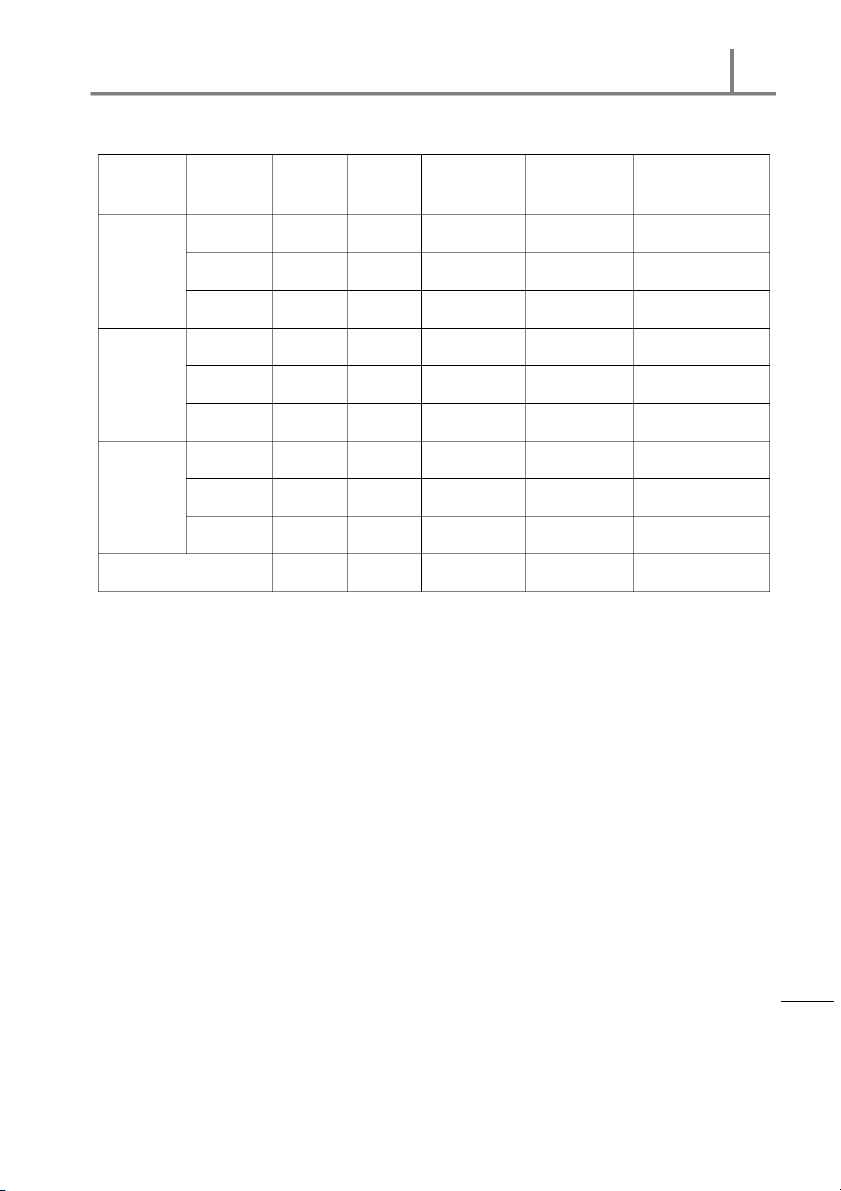
Table: Com put ing of Value of t he Chi – Square St at ist ic Habit of Regions O E O − E O Spending  − E
O− E/ E Nort her n 203 219.67 -16.67 277.89 1.27 < 50% Cent er 290 217.08 72.92 5,317.33 24.49 Incom e Sout hern 155 211.25 -56.25 3,164.06 14.98 Nort her n 266 239.67 26.33 693.27 2.89 50 - 80% Cent er 226 236.85 -10.85 117.72 0.50 Incom e Sout hern 215 230.48 -15.48 239.63 1.04 Nort her n 209 218.66 -9.66 93.32 0.43 > 80% Cent er 154 216.08 -62.08 3,853.93 17.84 Incom e Sout hern 282 210.27 71.73 5,145.19 24.47 Tot al (colum n) 2,000 2,000 87.90 sts e
The chi – square t est st at ist ic value for independence is T re a   u q X 
 =  O − E/ E = 87.90 i - S   h : C  4
Thus t he t est st at ist ic value is t oo large ( X = 87.90), we can strongly reject H at all level of  r 1
significance. It m eans t hat based on t he Chi – Square t est ing for independence, w e have enough te
evidence t o prove t hat t he regions of Viet nam and t he habit of spen ding m oney are independent of ap h each ot her. C ss | e sin u r B s fo istic tat S
Pow ered by statisticsforbusinessiuba.blogspot.com 7