Chapter 4b: Local search algorithms | Đại Học Nội Vụ Hà Nội

lOMoAR cPSD|5906219 0
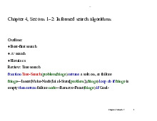
Chapter 4, Sec ons 3–4: Local search algorithms Outline ♦ Hill-climbing ♦ Simulated annealing
♦ Gene c algorithms (briefly)
♦ Local search in con nuous spaces (very briefly) Chapter 4, Sections 3–4 1 lOMoAR cPSD|590621 90
Iterative improvement algorithms
In many op miza on problems, path is irrelevant; the
goal state itself is the solu on
Then state space = set of “complete” configura ons; find
optimal configura on, e.g., TSP
or, find configura on sa sfying constraints, e.g., metable
In such cases, can use itera ve improvement algorithms; keep
a single “current” state, try to improve it
Constant space, suitable for online as well as offline search
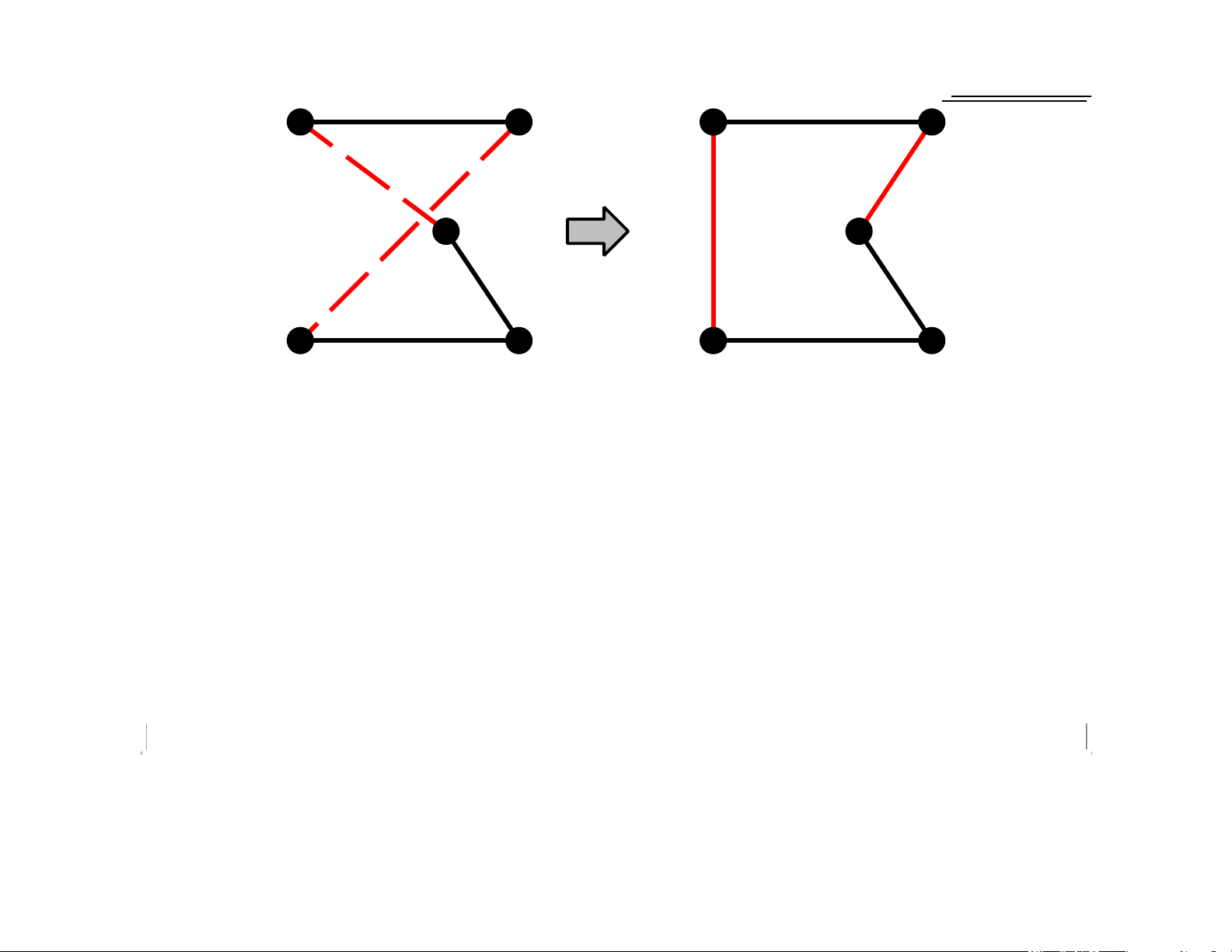
Example: Travelling Salesperson Problem
Start with any complete tour, perform pairwise exchanges Chapter 4, Sections 3–4 2 lOMoAR cPSD|590621 90 Chapter 4, Sections 3–4 3 lOMoAR cPSD|590621 90
Variants of this approach get within 1% of op mal very quickly with thousands of ci es Chapter 4, Sections 3–4 4 lOMoAR cPSD|5906219 0 Example: n-queens
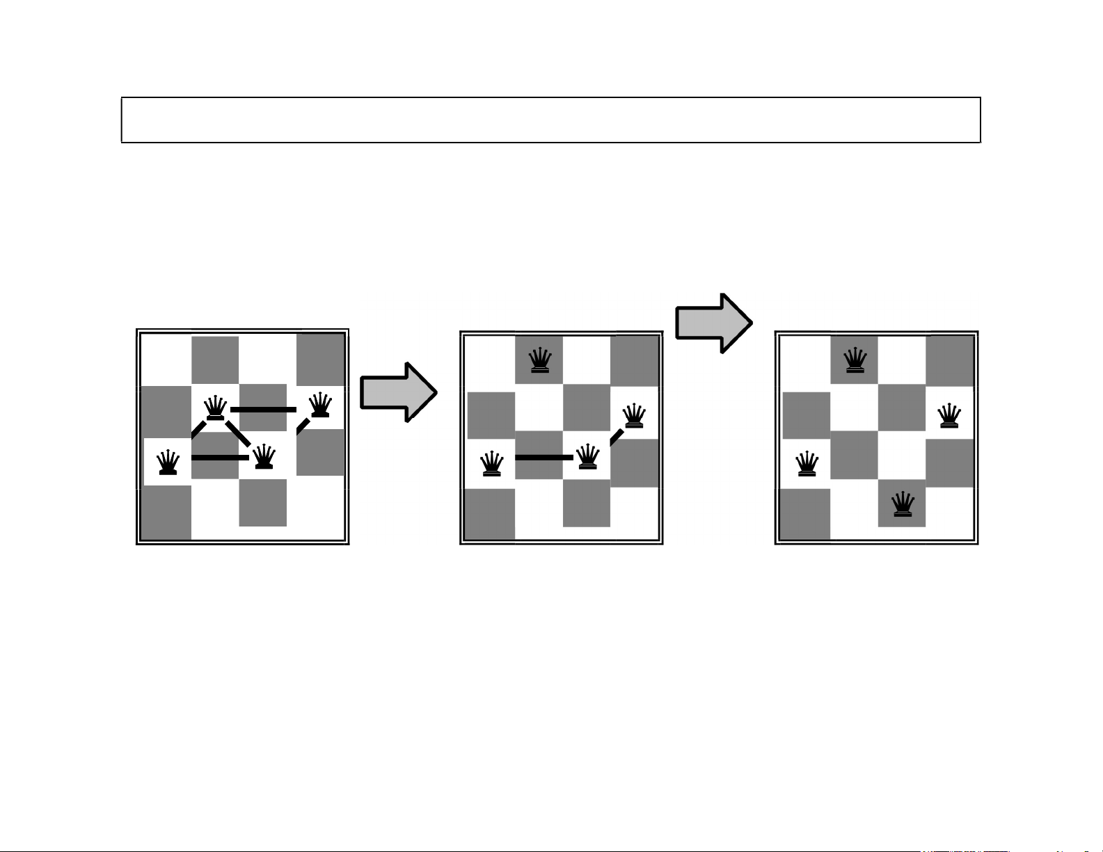
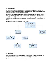
Put n queens on an n × n board with no two queens on the same row, column, or diagonal
Move a queen to reduce number of conflicts h = 5 h = 2 h = 0
Almost always solves n-queens problems almost instantaneously for
very large n, e.g., n=1million Chapter 4, Sections 3–4 5 lOMoAR cPSD|5906219 0
Hill-climbing (or gradient ascent/descent)
“Like climbing Everest in thick fog with amnesia”
func on Hill-Climbing(problem) returns a state that is a local maximum inputs:
problem, a problem local variables: current, a node neighbor, a node
current←Make-Node(Ini al-State[problem]) loop do neighbor← a
highest-valued successor of current if Value[neighbor] ≤
Value[current] then return State[current] current←neighbor end Hill-climbing contd. 6 lOMoAR cPSD|590621 90
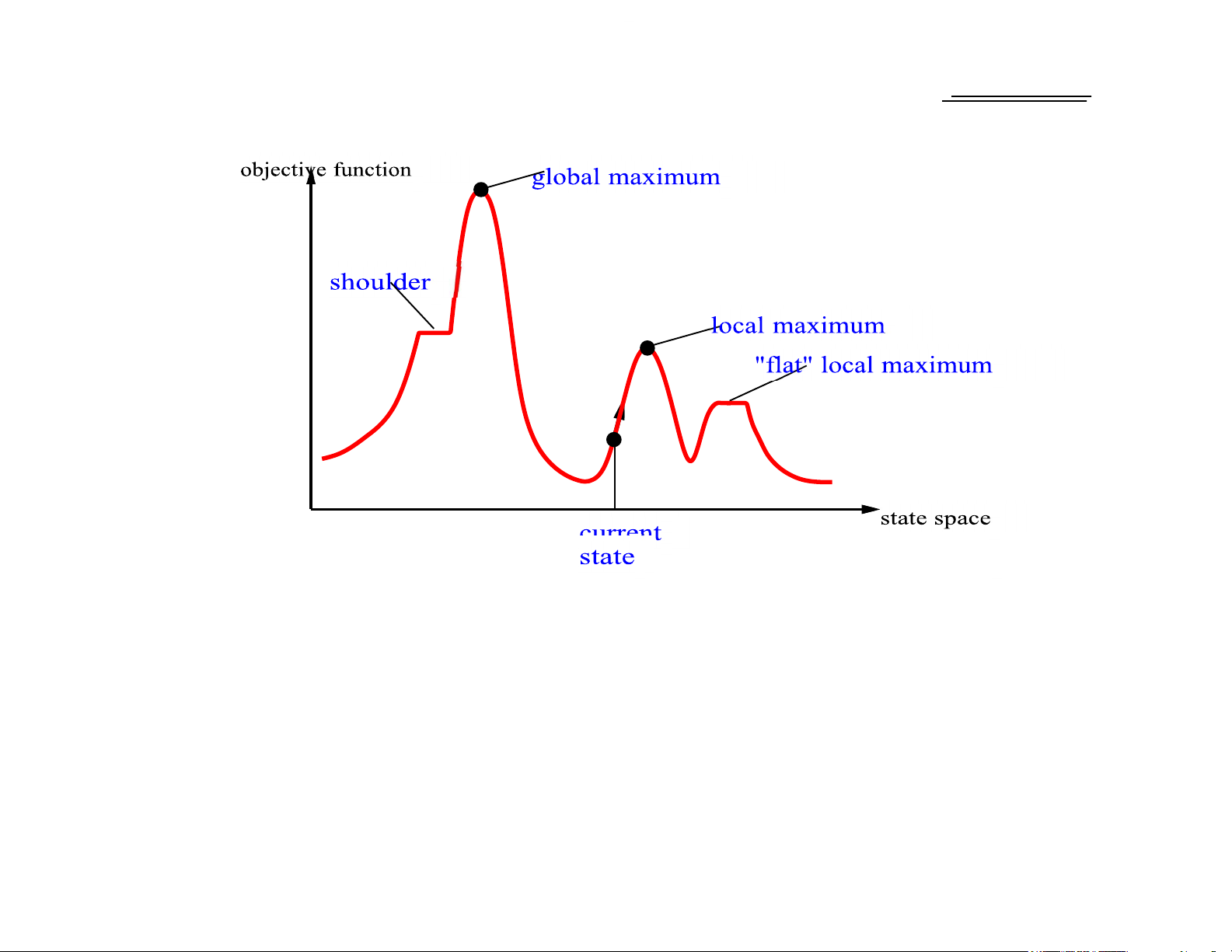
Useful to consider state space landscape
Random-restart hill climbing overcomes local maxima—trivially complete Chapter 4, Sections 3–4 7 lOMoAR cPSD|5906219 0 Chapter 4, Sections 3–4 Random sideways moves escape from shoulders loop on flat maxima 8 lOMoAR cPSD|590621 90 Simulated annealing
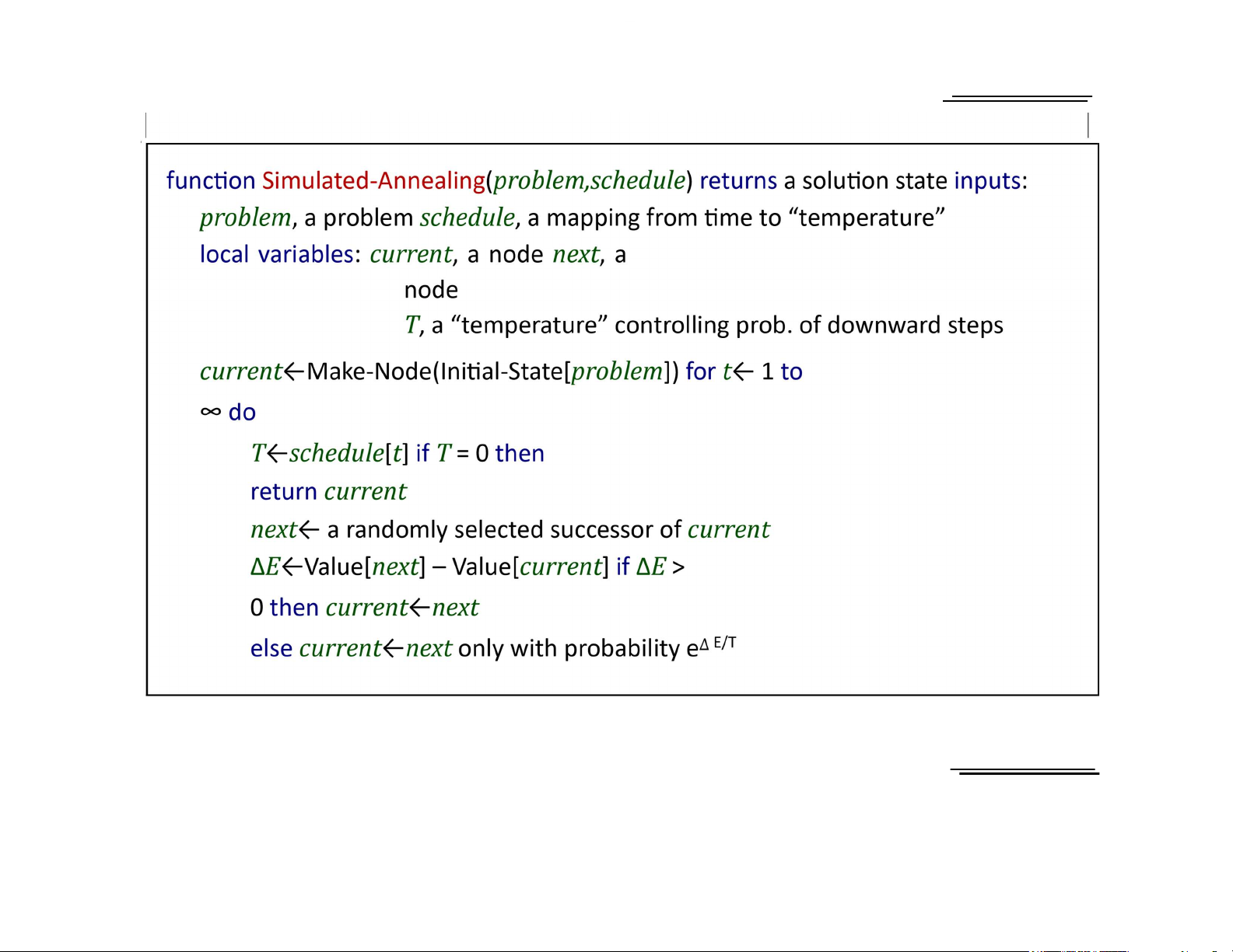
Idea: escape local maxima by allowing some “bad” moves but
gradually decrease their size and frequency Chapter 4, Sections 3–4 9 lOMoAR cPSD|590621 90
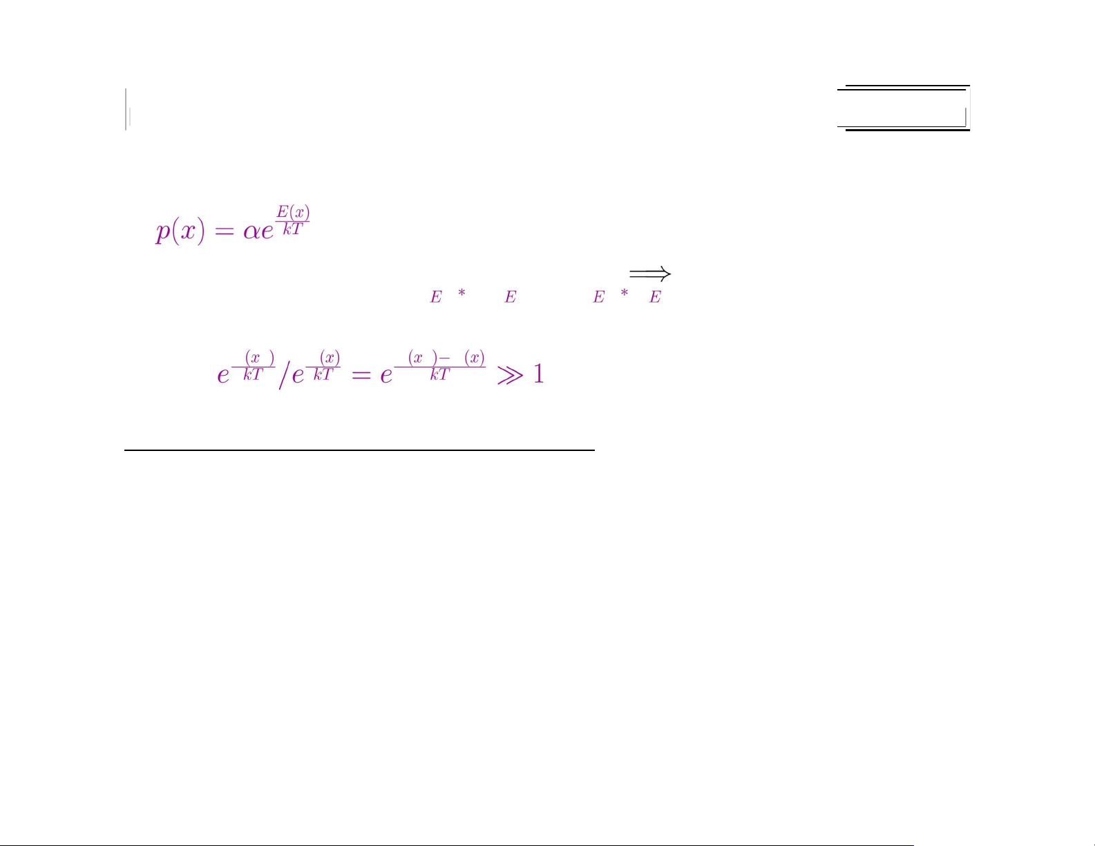
Properties of simulated annealing Chapter 4, Sections 3–4 10 lOMoAR cPSD|590621 90
At fixed “temperature” T, state occupa on probability reaches Boltzman distribu on T decreased slowly enough always reach best state x∗ because for small T
Is this necessarily an interes ng guarantee??
Devised by Metropolis et al., 1953, for physical process modelling
Widely used in VLSI layout, airline scheduling, etc. Local beam search
Idea: keep k states instead of 1; choose top k of all their successors
Not the same as k searches run in parallel! Chapter 4, Sections 3–4 11 lOMoAR cPSD|590621 90
Searches that find good states recruit other searches to join them
Problem: quite o en, all k states end up on same local hill Idea:
choose k successors randomly, biased towards good ones
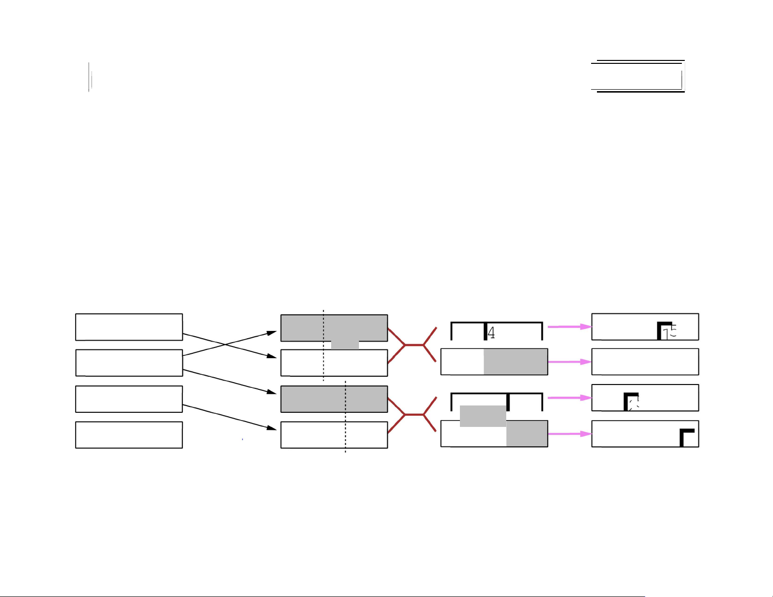
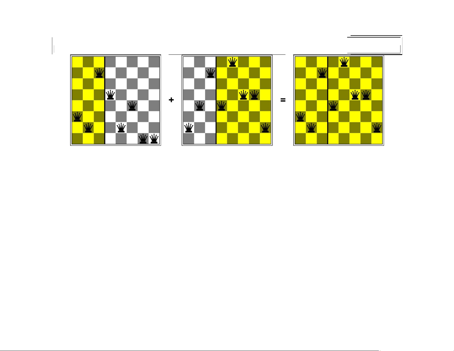
Observe the close analogy to natural selec on! Genetic algorithms
= stochas c local beam search + generate successors from pairs of states 24748552 24 31% 32752411 32748552 32748 152 32752411 23 29% 24748552 24752411 24752411 24415124 20 26% 32752411 32752124 32 252124 32543213 11 14% 24415124 24415411 2441541 7 Chapter 4, Sections 3–4 12 lOMoAR cPSD|590621 90 Fitness Selection Pairs Cross−Over Mutation Genetic algorithms contd.
GAs require states encoded as strings (GPs use programs)
Crossover helps iff substrings are meaningful components Chapter 4, Sections 3–4 13 lOMoAR cPSD|590621 90
GAs =6 evolu on: e.g., real genes encode replica on machinery! Continuous state spaces
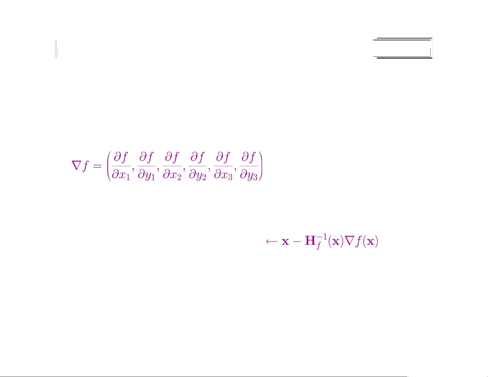
Suppose we want to site three airports in Romania:
– 6-D state space defined by (x1,y2), (x2,y2), (x3,y3) Chapter 4, Sections 3–4 14 lOMoAR cPSD|590621 90
– objec ve func on f(x1,y2,x2,y2,x3,y3) = sum of squared
distances from each city to nearest airport
Discre za on methods turn con nuous space into discrete space,
e.g., empirical gradient considers ±δ change in each coordinate Gradient methods compute
to increase/reduce f, e.g., by x ← x+ α∇f(x)
Some mes can solve for ∇f(x) = 0 exactly (e.g., with one city).
Newton–Raphson (1664, 1690) iterates x to
solve ∇f(x) = 0, where Hij =∂2f/∂xi∂xj Chapter 4, Sections 3–4 15