Chapter 6 The Market Structures | Bài giảng kinh tế học vi mô

Chapter 6: Market Structures Principles of Microeconomics By Tran Thi Kieu Minh, MSc Contents  Perfect Competition  Monopoly  Monopolistic Competition  Oligopoly 2
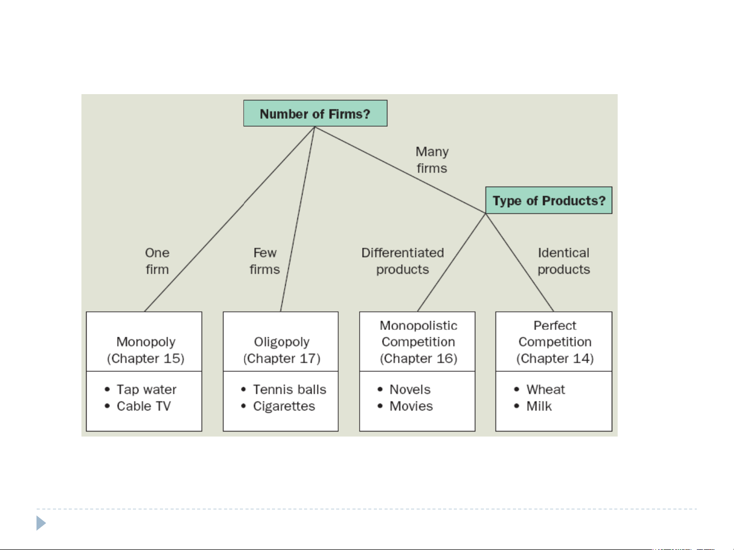
The four types of market structure
Economists who study industrial organization divide markets into four types:
monopoly, oligopoly, monopolistic competition, and perfect competition. 3 6.1 Competitive market Perfectly Competitive Markets Competitive Firm Profit Maximization
Competitive Market Supply Curve Chapter 14- Textbook 4
6.1.1 Perfectly Competitive Markets
 Competitive market: a market with many buyers
and sellers trading identical products so that each
buyer and seller is a price taker. 1. Price Taking 
The individual firm sells a very small share of the
total market output and the individual consumer
buys too small a share of industry output,
therefore, cannot influence market price. o have any impact on market price.  Price taker 2.
Product Homogeneity = identical products 
The products of all firms are perfect substitutes. 3. Free Entry and Exit 
Buyers can easily switch from one supplier to another. 
Suppliers can easily enter or exit a market. 5
Firms in the competitive market
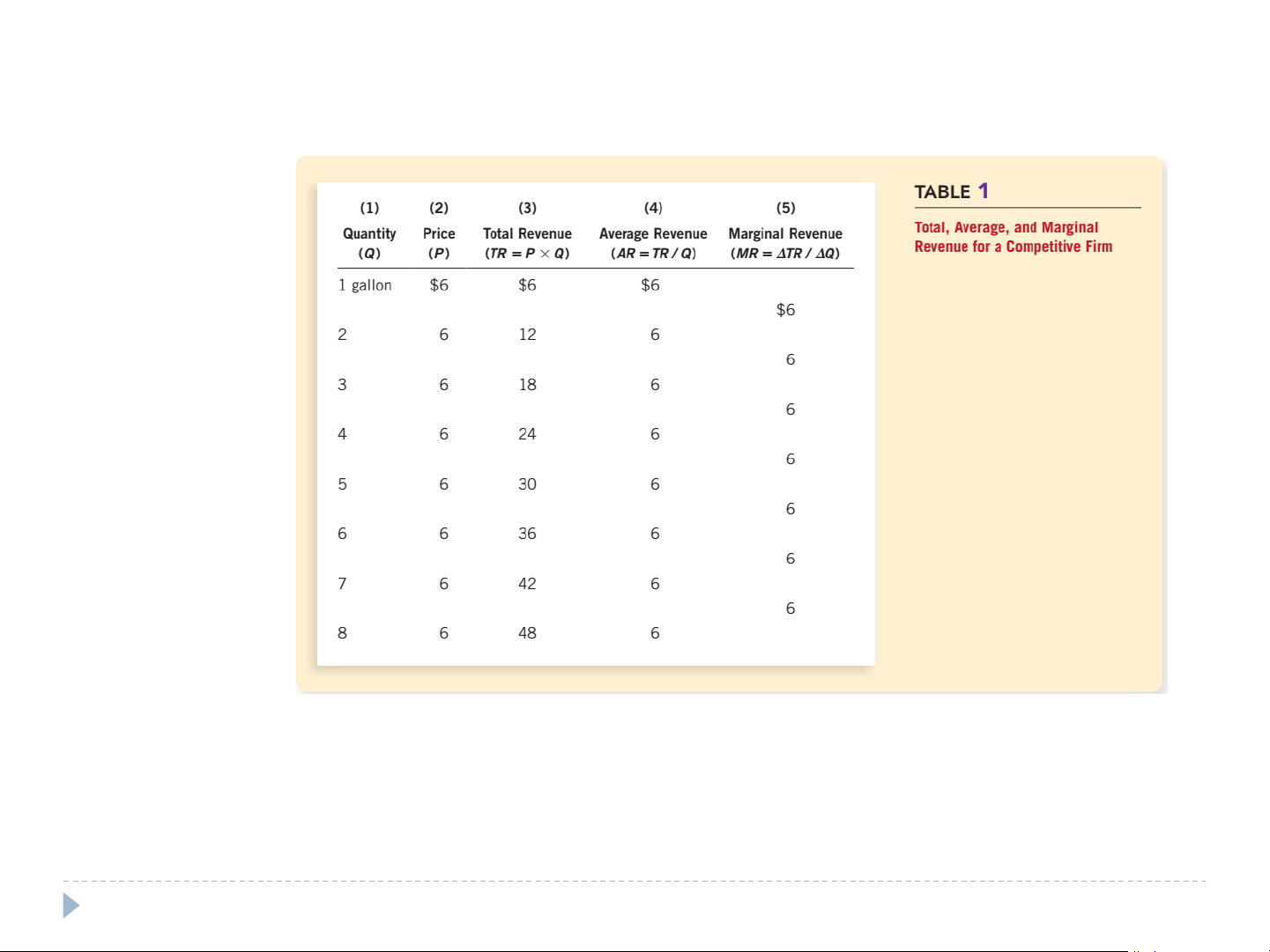
Table 1 shows the revenue for the Vaca Family Dairy Farm. Columns (1) and (2)
show the amount of output the farm produces and the price at which it sells its
output. Column (3) is the farm’s total revenue. 6
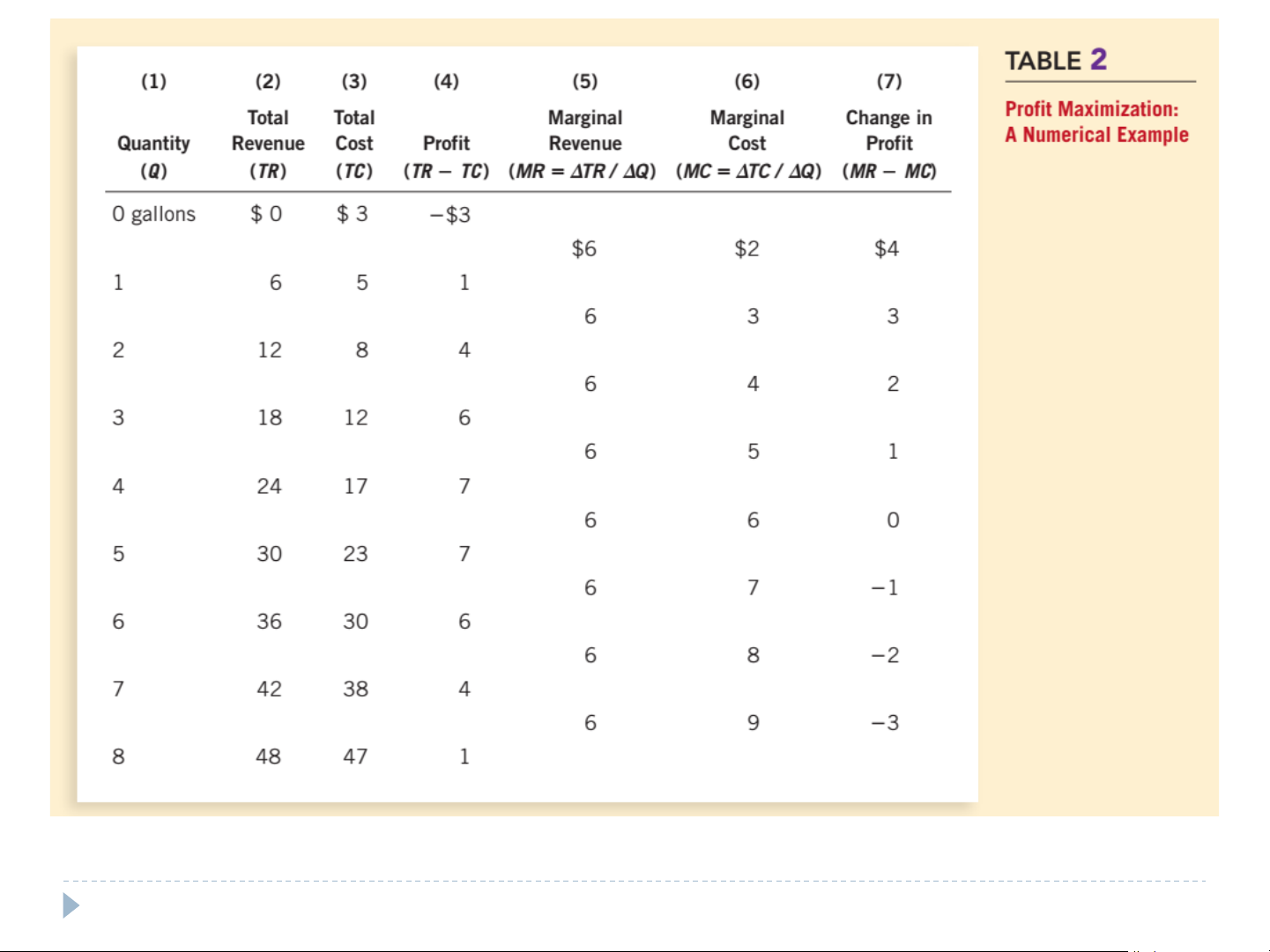
Vaca Farm’s decision: The Vacas can find the profit-maximizing quantity by
comparing the marginal revenue and marginal cost of each unit produced. 7 ©Kieu Minh, FTU
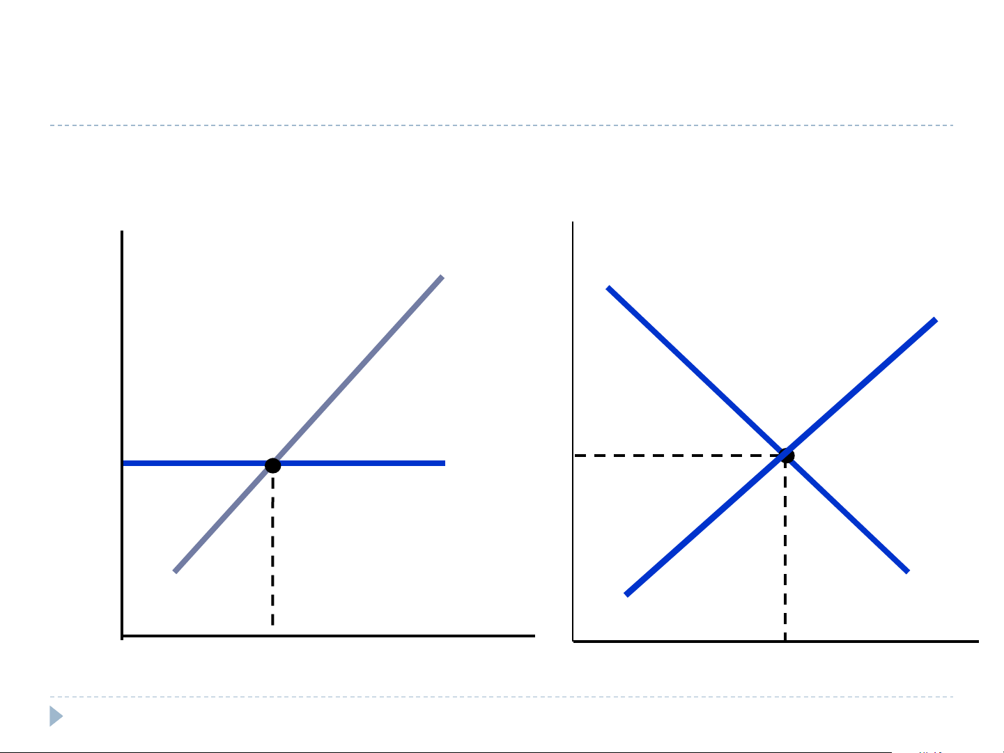
Firms in the competitive market Vaca Farm Milk Market Price $ per Price gallon $ per gallon MC S D=AR=MR $6 $6 D Output 5 Output 100 (gallons) (millions of gallons) 8
Competitive Firm’s optimum decision
 Demand curve faced by an individual firm is a horizontal line at the market price P
 Firm’s sales have no effect on market price  Average revenue: AR = P  Marginal revenue: MR = P  Profit Maximizing:
 For a perfectly competitive firm, profit maximizing output (q*) occurs when
MC(q) = MR = AR = P 9
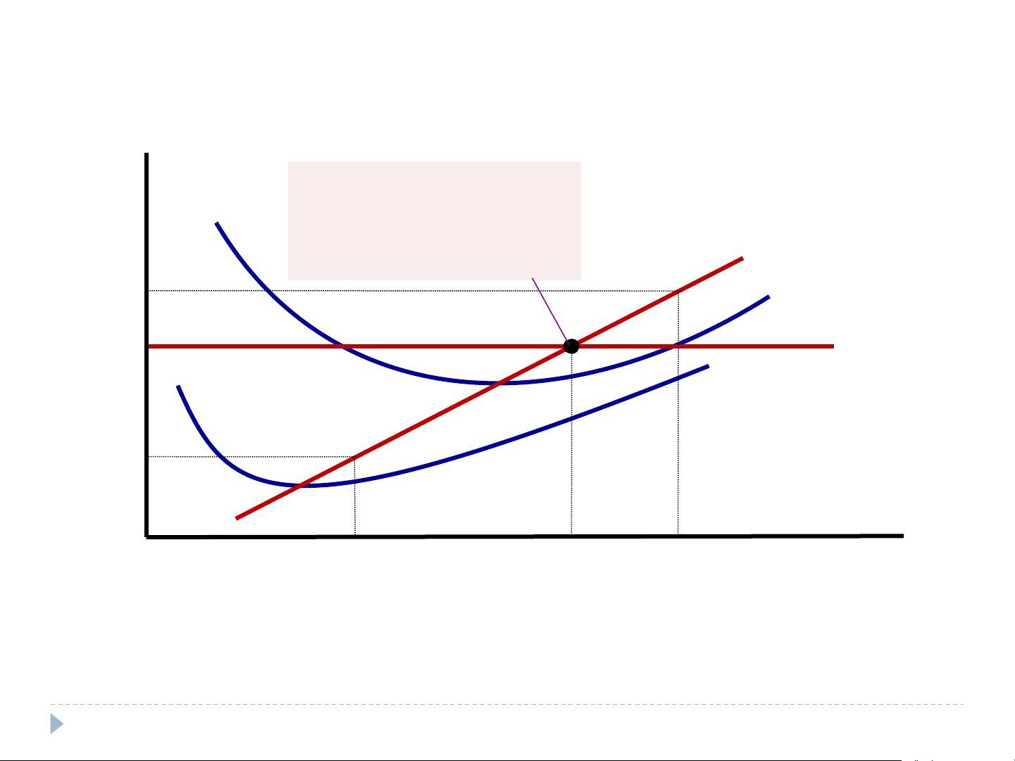
Profit maximization for a competitive firm Costs and The firm maximizes profit Revenue by producing the quantity at which marginal cost MC equals marginal revenue. MC ATC 2 P=MR =MR 1 2 P=AR=MR AVC MC1 0 Q Q 1 Q 2 Quantity MAX
At the quantity Q , marginal revenue MR exceeds marginal cost MC , so raising production 1 1 1
increases profit. At the quantity Q , marginal cost MC is above marginal revenue MR , so 2 2 2
reducing production increases profit. The profit-maximizing quantity Q is found where the MAX
horizontal price line intersects the marginal-cost curve. 10
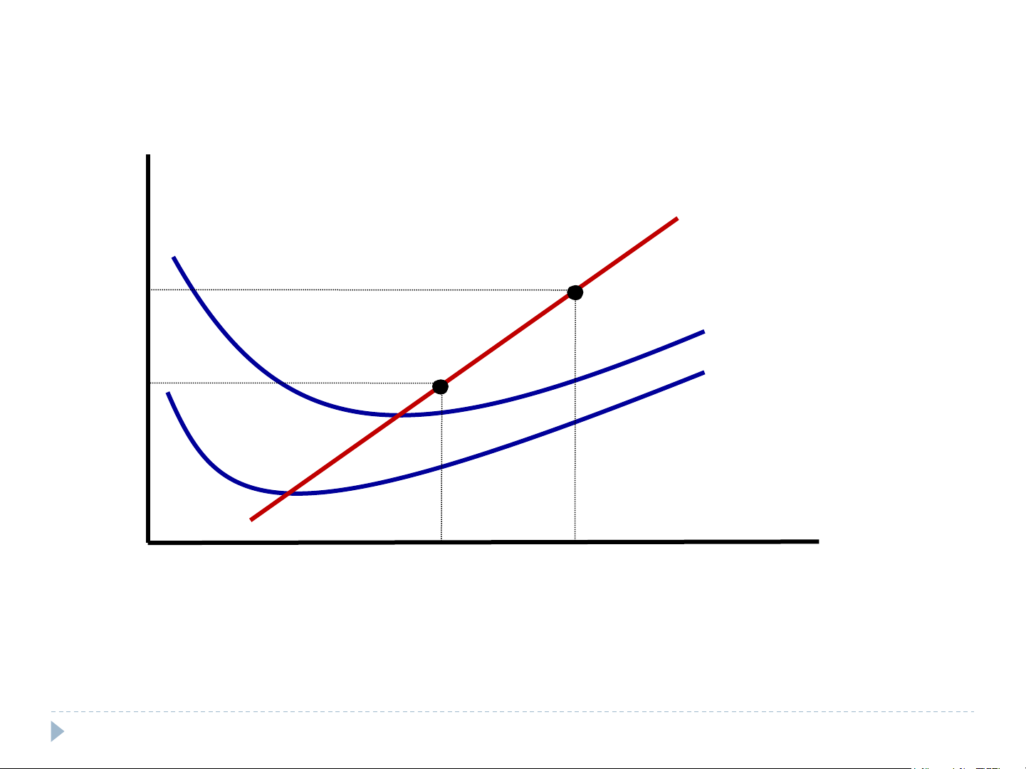
Marginal cost as the competitive firm’s supply curve Price MC P2 ATC P1 AVC 0 Q Q 1 2 Quantity
An increase in the price from P to P leads to an increase in the firm’s profit-maximizing 1 2
quantity from Q to Q . Because the marginal-cost curve shows the quantity supplied by 1 2
the firm at any given price, it is the firm’s supply curve. 11 Competitive Firm’s Decision
 The firm’s short-run decision to shut down
 Short-run decision not to produce anything during
a specific period of time because of current market conditions
 Firm still has to pay fixed costs
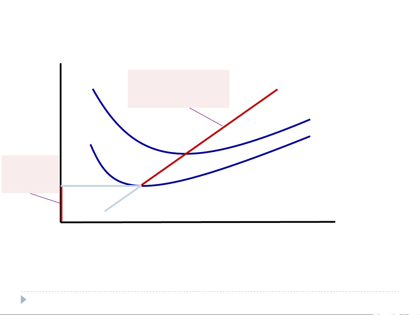
 Shut down if TR Competitive firm’s short-run supply curve
 The portion of its marginal-cost curve
 That lies above average variable cost (AVCmin) 12
The competitive firm’s short-run supply curve Costs 1. In the short run, the MC firm produces on the MC curve if P>AVC,... ATC AVC 2. ...but shuts down if P0 Quantity
In the short run, the competitive firm’s supply curve is its marginal-cost curve (MC) above
average variable cost (AVC). If the price falls below average variable cost, the firm is better off shutting down. 13
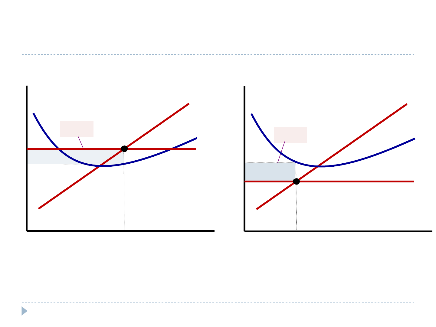
Profit as the area between price and average total cost (a) A firm with profits (b) A firm with losses Price Price MC MC Profit ATC Loss ATC P P=AR=MR ATC ATC P P=AR=MR 0 Q Quantity 0 Q Quantity (profit-maximizing quantity) (loss-minimizing quantity)  If P > ATC • If P < ATC
• Loss = TC - TR = (ATC – P) ˣ Q
 Profit = TR – TC = (P – ATC) ˣ Q = Negative profit 14
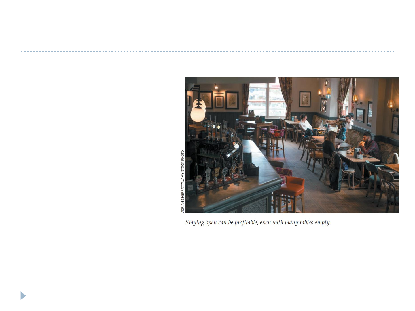
Case study: Near-empty restaurants
 Restaurant – stay open for lunch?  Fixed costs  Not relevant  Are sunk costs in short run
 Variable costs – relevant  Shut down if revenue from lunch < variable costs  Stay open if revenue from lunch > variable costs 15 Quiz 1
A competitive Firm ABC has average production cost ($) of 75
ATC = 2 + q + q a.
What is the marginal cost function of Firm ABC? b.
If market price is $30, what is the optimum quantity of
the firm? How much is the maximum profit? c.
What is the firm’s decision if market price decreases to $10? Explain. d.
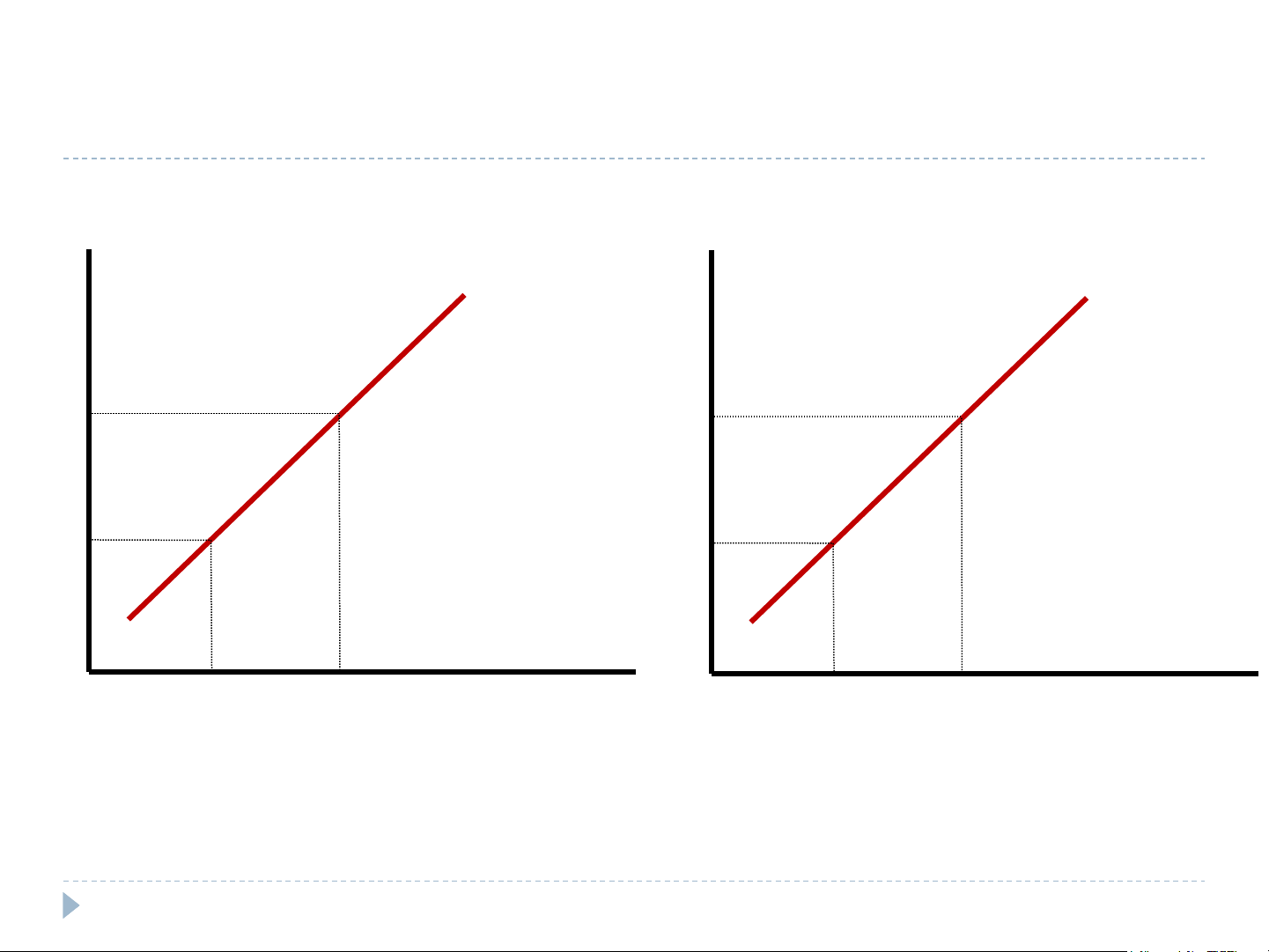
What is the short-run supply curve of the firm? e. How much is the ATCmin ? 16 Short-run market supply (a) Individual firm supply (b) Market supply Price Price MC Supply $2.00 $2.00 1.00 1.00 0 100 200 Quantity 0 100,000 200,000 Quantity (firm) (market)
In the short run, the number of firms in the market is fixed. As a result, the market supply curve,
shown in panel (b), reflects the individual firms’ marginal-cost curves, shown in panel (a). Here,
in a market of 1,000 firms, the quantity of output supplied to the market is 1,000 times the quantity 17 supplied by each firm. Quiz 2
A competitive market of a good A has 1000 similar sellers, each has production cost of: 1 2 TC = q − 5q + 8 2 = − Market demand of good A is : Q 20000 500P 1.
What is the suppy curve of one seller? 2.
What is the market supply curve of good A? 3.
What is the market equilibrium price and quantity? 4.
What is the optimum selling quantity of each seller? 18 19 6.2 Monopoly Monopolist
Demand and Marginal Revenue Profit maximization Market power Price discrimination Chapter 15- Textbook 20