Comparison of different methods to solve Electric Vehicle Routing Problem

1
Comparison of different methods to solve
Electric Vehicle Routing Problem
Huynh Do Anh Vu – 18521665@gm.uit.edu.vn, Pham Tien Trung – 18521558@gm.uit.edu.vn,
Nguyen Kieu Vinh – 18521653@gm.uit.edu.vn, Nguyen Anh Tuan – 18521600@gm.uit.edu.vn
Abstract— Our research studies the capacitated electric II. PROBLEM DEFINITION
vehicle routing problem (EVRP), is extended by the vehicle
The content of this section is mostly taken over from [1].
routing problem (VRP) and takes into account specific
The EVRP is a challenging NP-hard combinatorial
characteristics of electric vehicles. We formulate the
optimization problem as it is an extension of the ordinary
mathematical models of the EVRP and compare different
shortest path problem incorporating additional constraints. The
method to solve Electric Vehicle Routing Problem. The
EVRP can be described as follows: given a fleet of EVs, we
objective of the EVRP is to minimize the total distance
need to find the best possible route for each EV within their
traveled by an electric vehicle (EV). Our research conducts
battery charge level limits, starting and ending to the central
a numerical experiment and sensitivity analysis. The results
depot, to serve a set of customers. The objective is to minimize
of the numerical experiment show that these algorithms are
the total distance traveled, while each customer is visited
capable of obtaining good EVRP solutions within a
exactly once. And for each route in EV’s solution, the total
reasonable amount of time, and the sensitivity analysis
demand of customers does not exceed the maximum EV’s
demonstrates that the total distance is dependent on the
maximum carrying capacity and the total energy consumptions
number of customers, the vehicle driving range, battery
does not exceed the total maximum battery’s level. All EVs
charge level limits and maximum carrying capacity. Finally,
begin and end at the depot, EVs always leave the charging
method use MST as the base for Initial Construction
station fully charged (or fully charged and loaded if it goes from
method, combine with Randomized VND local search and
depot), and the charging station, including the depot, can be
AFS reallocation give better results than the other methods
visited multiple time. The charging station will be referred to as
in the most of benchmarks.
AFS for the rest of this paper.
The EVRP can be mathematically formulated as follows: I. INTRODUCTION min ∑ 𝑑𝑖𝑗𝑥𝑖𝑗, (1)
ransportation is the main contributor for CO2 waste,
𝑖∈𝑉,𝑗∈𝑉,𝑖≠𝑗
which causes global warming, pollution and climate
Tcha nges. Because of this, many logistic companies such (2)
as FedEx, UPS, DHL and TNT are investing in a way to reduce
∑ 𝑥𝑖𝑗 = 1, ∀𝑖 ∈ 𝐼,
the CO2 waste as a part of their daily operations. This makes 𝑗∈𝑉,𝑖≠𝑗
the importance of electric vehicles (EVs) increasing by the
recent years. The development of electric vehicles has
∑ 𝑥𝑖𝑗 ≤ 1, ∀𝑖 ∈ 𝐹′, (3)
progressed massively, and many of them have been put into use. 𝑗∈𝑉,𝑖≠𝑗
Although the electric vehicles have many advantages over the
traditional vehicles, such as independence of fossil fuels, etc…,
it still has one big disadvantage and that is the limited battery’s
∑ 𝑥𝑖𝑗 − ∑ 𝑥𝑗𝑖 = 0, ∀𝑖 ∈ 𝑉, (4)
capacity. This gives rise to the demand of new route planning 𝑗∈𝑉,𝑖≠𝑗 𝑗∈𝑉,𝑖≠𝑗
algorithms, which take into account the special properties of
EVs. This project is motived by the IEEE WCCI-2020
𝑢𝑗 ≤ 𝑢𝑖 − 𝑏𝑖𝑥𝑖𝑗 + 𝐶(1 − 𝑥𝑖𝑗), ∀𝑖 ∈ 𝑉, ∀𝑗 ∈ 𝑉, 𝑖 ≠ 𝑗, (5)
Competition on Evolutionary Computation for the Electric
Vehicle Routing Problem (EVRP) [1]. In this paper, we will
0 ≤ 𝑢𝑖 ≤ 𝐶, ∀𝑖 ∈ 𝑉, (6)
present the problem definition in Section II, all the related work
in for this problem in Section III. The method we used to solve
𝑦𝑗 ≤ 𝑦𝑖 − ℎ𝑑𝑖𝑗𝑥𝑖𝑗 + 𝑄(1 − 𝑥𝑖𝑗), ∀𝑖 ∈ 𝐼, ∀𝑗 ∈ 𝑉, 𝑖 ≠ 𝑗, (7)
this problem will be described in Section IV. Section V
discusses the experimental results. And finally, Section VI
𝑦𝑗 ≤ 𝑄 − ℎ𝑑𝑖𝑗𝑥𝑖𝑗, ∀𝑖 ∈ 𝐹′ ∪ {0}, ∀𝑗 ∈ 𝑉, 𝑖 ≠ 𝑗, (8)
presents conclusions and future direction.
0 ≤ 𝑦𝑗 ≤ 𝑄, ∀𝑖 ∈ 𝑉, (9) 2
𝑥𝑖𝑗 ∈ {0,1}, ∀𝑖 ∈ 𝑉, ∀𝑗 ∈ 𝑉, 𝑖 ≠ 𝑗,
(10) efficient strategy is to select a metaheuristic that has good
performance on the original VRP problem and can be easily
where 𝑉 = {0 ∪ 𝐼 ∪ 𝐹′} is a set of nodes and 𝐴 =
adapted with respect to the additional constraints of the EVRP.
{(𝑖, 𝑗)|𝑖, 𝑗 ∈ 𝑉, 𝑖 ≠ 𝑗} is a set of arcs in the fully connected
These two criteria are responsed by the metaheuristics
weighted graph 𝐺 = (𝑉, 𝐴). Set I denote the set of customers,
performing neighborhood-oriented, so we choose Randomized
set 𝐹′ denotes set of 𝛽𝑖 node copies of each charging station 𝑖 ∈ Variable Neighborhood Descent (RVND), Variable
𝐹 (i.e., |𝐹′| = ∑𝑖∈𝐹 𝛽𝑖) and 0 denotes the central depot. Then, Neighborhood Descent (VND) and Variable Neighborhood
𝑥𝑖𝑗 is a binary decision variable corresponding to usage of the Search (VNS) to solve this problem [13].
arc from node 𝑖 ∈ 𝑉 to node 𝑗 ∈ 𝑉 and 𝑑𝑖𝑗 is the weight of this
Local search is an integral part of these metaheuristics, it
arc. Variables 𝑢𝑖 and 𝑢𝑗 denote, respectively, the remaining
allows systematic search in a neighborhood of a current solution
carrying capacity and remaining battery charge level of an EV
using local search operators [11]. Local search operators are
on its arrival at node 𝑖 ∈ 𝑉. Finally, the constant ℎ denotes the described in Section IV-B.
consumption rate of the EVs, 𝐶 denotes their maximal carrying
Another problem is designing a method for the construction
capacity, 𝑄 the maximal battery charge level, and 𝑏𝑖 the demand
of a valid initial solution. Construction methods are described
of each customer 𝑖 ∈ 𝐼. in Section IV-C.
For formal components description, we define an EVRP tour
T as a sequence of nodes T = {v0, v1, ..., vn−1}, where vi is a III. RELATED WORK
customer, a depot or an AFS and n is the length of the tour T. Then, let e
According to the [1], the EVRP variant was first solved in [2].
ij be an edge from node vi to node vj and wi,j be its weight.
As far as we are concerned, only three papers are dealing with
this problem, and for each one of them, the exact problem A. Metaheuristic
formulation slightly varies. The first one is [3], which limits the
1) (Randomized) Variable Neighborhood Descent -
maximum number of routes in addition to the previously
(R)VND: VND is a simple metaheuristic used as a local search
introduced constraints. It presents the solution method based on
method in a more complex metaheuristic VNS (Section IV-A2).
the ant colony system (ACS) algorithm. Initially, a Travelling
It include a deterministic variant (VND) and a stochastic one
Salesman Problem (TSP) route visiting all customers is
(RVND). The input is a valid EVRP tour T , a sequence of local
constructed. This route is then turned into a valid EVRP route
search operators N, and a maximum number of fitness
by a newly proposed fixing method. Then, the ACS modifies evaluations evals [5] max
. The operators passed in N are described
the underlying TSP route according to the solution fitness score, in Section IV-B.
and the whole process repeats.
The VND algorithm requires an input as an initial vaild
The second one is [4], which also considers the maximum
solution and will output a vaild EVRP tour that has fitness equal
total delivery time on top of the previously introduced
or better than the initial solution. At each iteration, a local
constraints. The initial valid EVRP tour is constructed from the
search operator with the first improvement strategy (excluding
nearest neighbor based TSP tour visiting all customers. The
AFS reallocation) is applied to a solution. The search continue
solution is then improved in a local search phase while using
in the next neighborhood until an improvement is found.
four different neighborhood operators (swap, insert, insert AFS,
Both of VND and RVND perform the local search (according
and delete AFS). The proposed algorithm uses a simulated
to the best-improvement scenario) sequentially following the operator’s order
annealing mechanism to allow for accepting non-improving
in N. In the case of the RVND, the order of the
operators is randomly shuffled first, whereas in the VND, the
moves with a certain probability, thus preventing premature
order remains fixed. Each time an improvement is made, the
convergence to a local optimum.
local search is restarted. The VND then starts again from the
Finally, [5] proposes a novel construction method and a
first operator in N, while the RVND randomly reshuffles all
metaheuristic algorithm consisting of a local search and a
operators first. The algorithm terminates either when no
metaheuristic algorithm. The local search combines the
improvement is achieved in any of the operators or when a stop
Variable Neighborhood Search (VNS) with Randomized condition is met [5].
Variable Neighborhood Descent (RVND). The operators used
2) Variable Neighborhood Search (VNS): VNS is a
in the local search are 2-opt, 2-string, and AFS reallocation.
metaheuristic method which is commonly used to find sub-
Various other approaches were successfully applied to the
optimal solutions of optimization problems such as the VRP. It
numerous variants of the VRP, and many of these can be
systematically changes the searched neighborhood in two
adapted to the EVRP formulation. For example, a survey [6]
phases: an exhaustive local search to reach a local optimum and
focused only on the variants of EVRP.
a perturbation phase, which uses to get out of the corresponding valley. IV. METHODS
First, an initial solution is constructed using one of the
construction methods described in Section IV-C. Then, the
NP-hard is impossible to solve in the larger instances in a
following process repeats. The best known solution T* is
reasonable time. In order to tackle this problem, we deployed a
modified by a randomized perturbation, which results in a
metaheuristic approach with polynomial time complexity. The
possibly non-improving current solution T. The current solution
EVRP is a constrained variant of the VRP. In those case, an
T then passes through a systematic local search, which uses the 3
operators described in Section IV-B. These operators in the
input and returns a modified tour 𝑇’, where the sequence of
local search phase are applied according to the VND or RVND
nodes from 𝑖 to 𝑗 index is reversed. It must hold, that 𝑖 < 𝑗, 𝑖 ≥
metaheuristics. If the cost of the current solution T is better than 1 and 𝑗 < 𝑛.
the cost of T*, T* replaces T as the new best solution. The
The cost update function δ2−𝑜𝑝𝑡 can be evaluated as:
search process terminates when a stop condition is met. The
EVRP competition defines it as a maximal number of fitness
δ2−𝑜𝑝𝑡 = 𝑤𝑖−1,𝑖 + 𝑤𝑗,𝑗+1 − 𝑤𝑖−1,𝑗 − 𝑤𝑖,𝑗+1 (11)
function evaluations. When this number is reached within the
local search, it terminates and sets the stop flag to true, thus
where the indices are expressed with respect to the tour T. terminating the VNS loop.
The perturbation operator is intended to move the search 2) Or-opt:
process out of the reach of the local search operators while
Our Or-opt is a special case of 2-opt in which two adjacent
keeping most of the properties of the current best solution T*.
nodes from two different location will be swapped in the tour.
For this purpose, the Double-Bridge perturbation is used. The
It takes a pair of indices 𝑖, 𝑗 and a tour 𝑇 as an input and returns
Double-Bridge splits the best known solution T* into p + 1
a modified tour 𝑇’, where the adjacent node (𝑖, 𝑖 + 1) and (𝑗, 𝑗 +
subroutes, with p is randomly selected indices. These subroutes
1) are swapped. It must hold, that 𝑖 + 1 < 𝑗, 𝑖 ≥ 1 and 𝑗 <
are randomly shuffled, inverted, and reconnected, producing a 𝑛 − 2.
possibly invalid tour. This tour is then repaired if necessary by
the SSF construction described in IV-C and passed to the local
The cost update function δor−opt can be evaluated as:
search as a valid tour T. B. Local Search
δ𝑜𝑟−𝑜𝑝𝑡 = 𝑤𝑖−1,𝑖 + 𝑤𝑖+1,𝑖+2 + 𝑤𝑗−1,𝑗 + 𝑤𝑗+1,𝑗+2 −𝑤
Local search is one of few general approaches to
𝑖−1,𝑗 − 𝑤𝑗+1,𝑖+2 − 𝑤𝑗−1,𝑖 − 𝑤𝑖+1,𝑗+2 (12)
combinatorial optimization problems. The basic idea of local
search is that high-quality solutions of an optimization problem 3) Exchange:
can be found by iteratively improving a solution using small
The exchange operator behaves similar to the Or-opt
modifications, called moves. A local search operator specifies
operator, but only move one node instead of moving two
a move type and generates a neighborhood from the current
adjacent nodes. It takes a pair of indices 𝑖, 𝑗 and a tour 𝑇 as an
solution. Given the solution s, the neighborhood of a local
input and returns a modified tour 𝑇’, where the node 𝑖 and 𝑗 are
search operator is the set of solutions N(s) that can be
swapped. It must hold, that i < 𝑗, 𝑖 ≥ 1 and 𝑗 < 𝑛 − 1.
reached from s by applying a single move of that type. After
generating the neighborhood of the current solution, the
The cost update function δexchange can be evaluated as:
neigborhood is evaluated, and local search uses a move strategy
to select at most one solution from the neighborhood N(s) to
δ𝑒𝑥𝑐ℎ𝑎𝑛𝑔𝑒 = 𝑤𝑖−1,𝑖 + 𝑤𝑖,𝑖+1 + 𝑤𝑗−1,𝑗 + 𝑤𝑗,𝑗+1
become the next current solution [11]. The move strategy we
−𝑤𝑖−1,𝑗 − 𝑤𝑗,𝑖+1 − 𝑤𝑗−1,𝑖 − 𝑤𝑖,𝑗+1 (13)
used is called steepest descent, it selects the solution from the
neighborhood with the best objective function value, provided 4) Relocate:
that this solution is better than the current solution. If there is
Changing the order of nodes can produce different solutions.
no better solution in the neighborhood than the current solution
Relocate is the process where a selected node is moved from its
then the local optimum has been reached [13].
current position in the tour to another position. Hence, the
In general, local search operators for the EVRP can be
position of the selected node is relocated. Each relocation of a
distinguished between operators for intra-route optimization
node produces one outcome [12]. It takes a pair of indices 𝑖, 𝑗 and
and operators for inter-route optimization. These two operator
a tour 𝑇 as an input and returns a modified tour 𝑇’, where the
types reflect the two tasks that one has to solve in a EVRP: The
node 𝑖 is removed and inserted to index 𝑗. It must hold, that i <
allocation of customers to routes (inter-route optimization), and
𝑗, 𝑖 ≥ 1 and 𝑗 < 𝑛.
the optimization of each route in itself (intra-route
optimization) [11]. These two tasks do not necessarily have to
The cost update function δrelocate can be evaluated as:
be solved in this order, nor sequentially.
The cost update functions δ provided are expressed as a
δ𝑟𝑒𝑙𝑜𝑐𝑎𝑡𝑒 = 𝑤𝑖−1,𝑖 + 𝑤𝑖,𝑖+1 + 𝑤𝑗−1,𝑗
difference between the sum of removed edges weights and the
−𝑤𝑖−1,𝑖+1 − 𝑤𝑗−1,𝑖 − 𝑤𝑖,𝑗 (14)
sum of newly added edges weights. Thus, a positive value of
the cost update corresponds to an improvement in fitness and 5) AFS reallocation:
vice versa. Only first improvement mode was tested in the local
This operator will rearrange and remove the duplicate nodes
search. In the first improvement, the first improving tour found
in the valid EVRP tour. The duplicate nodes are the nodes that
is accepted, and the search in the current neighborhood is
are continuously identical in the tour. First all the AFS and
terminated. In both cases, only valid tours are accepted.
duplicate node in the tour are removed. Then the modified tour 1)
will pass through SSF (see Section IV-C2) to produce a valid 2-opt:
EVRP tour. This is the only operator that doesn’t have a cost
The idea of 2-opt is to remove two edges from the considered function.
route and replace them by two new edges, such that a new route
is formed [12]. It takes a pair of indices 𝑖, 𝑗 and a tour 𝑇 as an 4
C. Initial constructions:
number of AFSs varies. Because of the time constraint on the
The process to create a vaild EVRP tour includes two phase:
project, we only perform experiment on the E instances. The
initial construction and repair procedure [5]. In the first phase, a
detailed description for the problems is found in [1].
TSP feasible solution is created and go through all customer,
Because the implemented metaheuristic is stochastic,
disregarding the capacity and battery’s level cosntraints,
according to the rules of the competition, we must run 20
starting from and ending with depot. This phase we will use
independent runs with random seeds from 1 to 20 for each run.
three algorithm to generate the solution: Nearest Neighbour
The stop condition for each run is defined by the maximum
(NN), Clarke-Wright Savings (CWS) and Minimum Spanning
number of evaluations with respect to problem size as
Tree (MST). The second phase we will use our developed
𝑒𝑣𝑎𝑙𝑠𝑚𝑎𝑥 = 25000𝑛 evaluations, where n is the problem size.
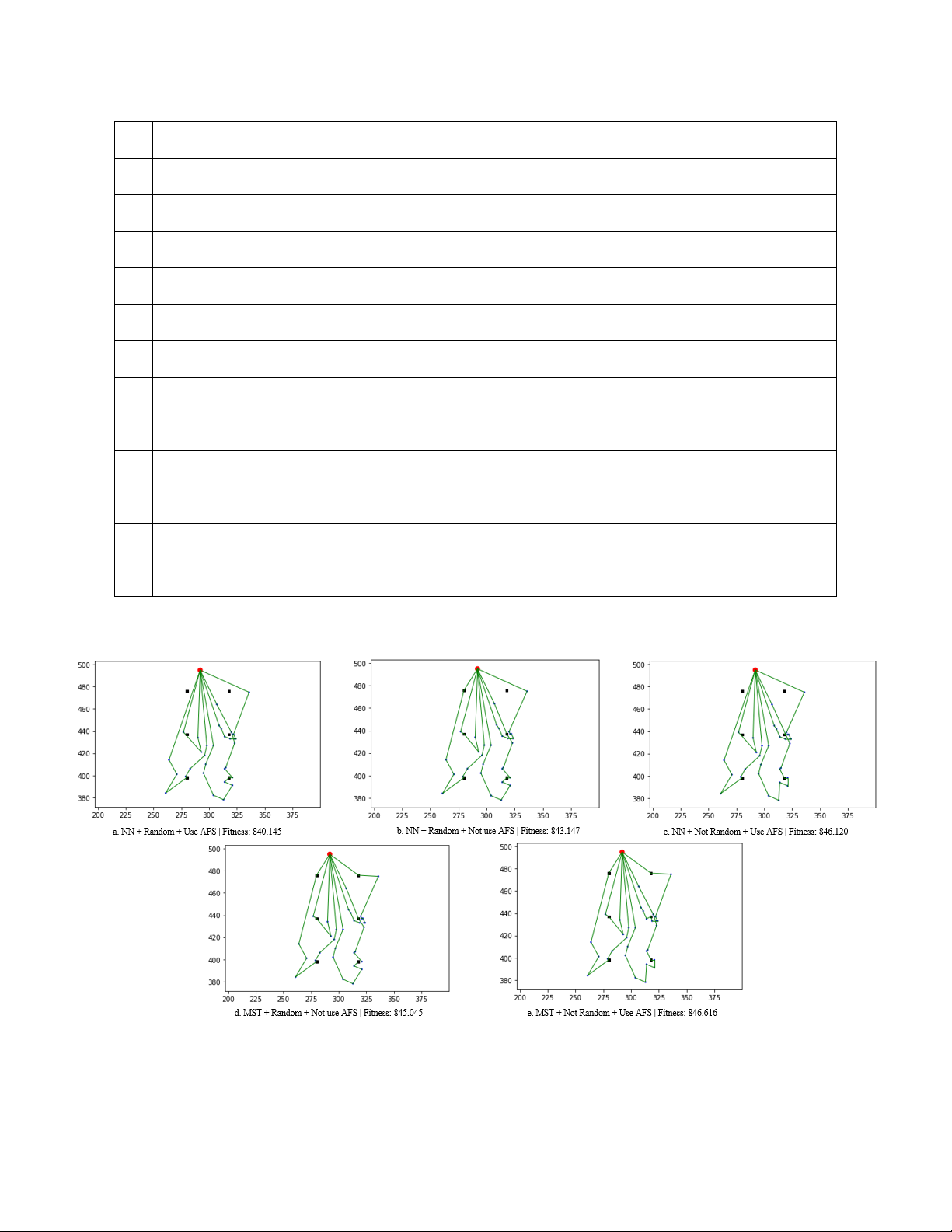
method to fix the TSP tour into a vaild EVRP tour. Several
In this section, we perform the experiment to see which
examples of generated EVRP tours are presented in Figure 1.
combination of setup give the best fitness value to the
1) Method to construct Initial TSP feasible solution:
problem’s instances. The fitness values will be the mean value
of the first 20 run. Benchmark values of tour fitness were a)
Nearest Neighbour (NN): The ideal behind this
provided in each instances files, however, these values are not
algorithm is rather simple. Starting from depot,
guaranteed to be optimal. In fact, in some of the instances, some
the algorithm will choose the next closest
of our method outperform the provided values.
customer that has not been visited. Repeat this
The setup can be broken down to three parts: Initial
process until all customers have been visited.
Construction method, Randomized or Sequential Local Search
After that we just need to add a depot at the end
and finally Use or Not use AFS reallocation as operator on [8]. Local Search.
B. Results and Discussion: b)
Clarke-Wright Savings (CWS): This is the most
Table I shows a comparison of generated EVRP tour’s
widely known heuristic algorithm for travelling
fitness values under different setup, averaged over the first 20
salesman problem or classical vehicle routing
run for each problem’s instances. All 12 setup generate a valid
problem. The concept of this algorithm is to solution for all instances.
determine the routes by the savings list in which
In the Table I, we see that over all the setups use AFS
values are sorted from largest to smallest [9].
reallocation as operator have fitness value higher than the
setups that don’t use. This happened because when the new c)
Minimum Spanning Tree (MST): The concept of
solution is found, it has already passed through all local search
this algorithm is to create a graph such that it
operators and possibly creates a path that is valid and better than
connects all the nodes (customers and depot),
the current solution, but if the current path has redundant AFS
without any circle and with the minimum sum
then the new path will also have those AFS as there is currently of edge weight [10].
no operator to remove them. That is why adding AFS
reallocation as an operator will help increase the solution’s
2) Separate Sequential Fixing (SSF): After the initial quality.
construction has been created using one of the methods above,
Moreover, the setups that use Randomized variant of VND
the TSP feasible solution then will be repaired to create a valid
have the better fitness value than the Sequential variant. We
EVRP solution. SSF splits into two phases. In the first phase,
suspect that this is because of the first improvement strategy in
the load constraint is checked sequentially and whenever the
local search operator. By using this strategy, only the first
next customer’s demand is not satisfied, a depot is inserted
improvement in cost will be accepted. This helps reduce the
before them. This will ensure the load constraint is always
complexity of the search and if given enough time and resource,
satisfied before moving to the next phase. In the second phase,
it will converge to local minima. However, the resource we had
SSF makes sure that the current node and the next node (it can
is limited so using Sequential variant of VND is not very
either be the depot, customer or AFS) can reach the nearest AFS
efficient. Instead, using a random operator for every local
of its own. If the next node can’t be reached, then the former
search call is a better choice because by using random operator,
one will ensure that there’s always a AFS nearby to add. But if
if we are lucky, then we will converge much faster than
the next node can’t reach its nearest AFS, then it will be stuck Sequential one.
in an infinite cycle of going back and forth. Thus, the latter one
And finally, using three method NN, CWS and MST as our
will break this infinite cycle by adding the next node’s nearest
base for comparison, it seems that the fitness value of three
AFS to the tour as next node. After passing through two phases,
methods above seems to differ between each setup and give no
the final route will be a valid EVRP tour. improvement in our solution.
It seems that the fitness value depends strongly on second
and third path and not depends on the method of initial V. EXPERIMENTS construction.
As shown in the Table I, the current best setup is setup 9, A. Benchmark Settings:
which use MST as the base for Initial Construction method,
A benchmark of 17 EVRP instances was provided in this
combine with Randomized VND local search and AFS
competition. These instances are split into two set small (E) and reallocation
large (X). Each instances contain exactly one depot, while the 5
VI. CONCLUSION AND FUTURE DIRECTION
[11] F. Arnold, K. Sorensena, Knowledge-guided local search for the Vehicle
Routing Problem, Univ. Antwerp, Departement of Engineering
In this paper, we do various experiments on different setup
Management, ANT/OR - Operations Research Group, May 2019.
to determine which setup is the best for the EVRP problem.
[12] L.Sengupta, R. Mariescu-Istodor, P. Fränti, Which Local Search
As mentioned in Section V-B, the current best setup is setup
Operator Works Best for the Open-Loop TSP?, Univ. Eastern Finland,
80101 Joensuu, Finland, 23 Sep. 2019.
9. The construction and local search are paired in the VNS
[13] A. Dhahri, A.Mjirda, K. Zidi, K. Ghedira, A VNS-based heuristic for
metaheuristic, which repeatedly performs Double Bridge
solving the vehicle routing problem with time windows and vehicle
perturbation and RVND until the stop condition is reached.
preventive maintenance constraints, ICCS 2016.
Various setups are also tested and implemented, although all the
setup we tested still fall far behind the top result in this problem
Huynh Do Anh Vu is a student in
as given in [7]. However, we still get some interesting results
University of Information Technology
when experimenting will the different setup.
(UIT) since 2018. His major is Computer
As mentioned in Section IV-A, we only run the E-instances
Science, he is currently at the third year
in this problem due to time constraint and we are fully aware
and he is in class KHCL2018.3. He is a
that this will not give a full insight on the comparison. In the
graduated high school student from THPT
future, we will perform experiment on the X-instances, Phu Nhuan, HCM.
implement more repair and initial construction methods for
comparison and conduct experiments on more metaheuristic algorithm.
Pham Tien Trung is a student in
University of Information Technology
(UIT) since 2018. His major is Computer R
Science. He is a class president in class EFERENCES
KHCL2018.3 and an executive committee
[1] Michalis Mavrovouniotis, Charalambos Menelaou, Stelios Timotheou,
of Computer Science faculty. He is a
Christos Panayiotou, Georgios Ellinas, and Marios Polycarpou,
Benchmark Set for the IEEE WCCI-2020 Competition on Evolutionary
graduated high school student from THPT
Computation for the Electric Vehicle Routing Problem, Tech. report, No 1 Tu Nghia, Quang Ngai.
KIOS Research and Innovation Center of Excellence, Department of
Electrical and Computer Engineering, University of Cyprus, Nicosia, Cyprus, 2020.
[2] F Goncalves, Cardoso S., and Relvas S., Optimization of distribution
Nguyen Kieu Vinh is a student in
network using electric vehicles: A VRP problem, Tech. report, University
University of Information Technology of Lisbon, 2011.
(UIT) since 2018. His major is Computer
[3] Shuai Zhang, Yuvraj Gajpal, and S. S. Appadoo, A meta-heuristic for
Science, he is currently at the third year
capacitated green vehicle routing problem, Annals of Operations
Research 269 (2018), no. 1-2, 753–771.
and he is in class KHCL2018.3. He is a
[4] Nur Mayke Eka Normasari, Vincent F. Yu, Candra Bachtiyar, and
graduated high school student from THPT
Sukoyo, A simulated annealing heuristic for the capacitated green
Nguyen Trung Truc, Kien Giang.
vehicle routing problem, Mathematical Problems in Engineering 2019 (2019).
[5] David Woller, Václav Vávra and Viktor Kozák, Electric Vehicle Routing Problem.
[6] Tomislav Erdelic, Tonci Caric, and Eduardo Lalla-Ruiz, A Survey on the
Nguyen Anh Tuan is a student in
Electric Vehicle Routing Problem: Variants and Solution Approaches,
University of Information Technology 2019.
[7] KIOS, CEC-12 Competition on Electric Vehicle Routing Problem, July
(UIT) since 2018. His major is Computer
19-24,2020,Glasgow,Scotland,U.K.
Science, he is currently at the third year and
https://mavrovouniotis.github.io/EVRPcompetition2020/
he is in class KHCL2018.3. He is a
[8] Wikipedia, Nearest neighbour algorithm, 28 February 2021.
graduated high school student from THPT
https://en.wikipedia.org/wiki/Nearest_neighbour_algorithm
[9] Tantikorn Pichpibul and Ruengsak Kawtummachai, New Enhancement Di Linh, Lam Dong.
for Clarke-Wright Savings Algorithm to Optimize the Capacitated
Vehicle Routing Problem, European Journal of Scientific Research ISSN 1450-216X Vol.78 No.1 (2012). [10] Wikipedia, Minimum spanning tree, 6 July 2021.
https://en.wikipedia.org/wiki/Minimum_spanning_tree 6 E-n22- E-n23- E-n30- E-n33- E-n51- E-n76- E-n101- No Setup k4.evrp k3.evrp k3.evrp k4.evrp k5.evrp k7.evrp k8.verp NN + Random + 1 384.678 571.947 509.470 840.237 535.235 705.678 858.524 Use AFS NN + Random + 2 394.174 581.505 520.905 845.034 539.373 709.157 858.626 Not use AFS NN + Sequence + 3 385.406 578.827 520.303 848.324 544.196 720.711 873.871 Use AFS NN + Sequence + 4 396.022 581.936 520.303 847.767 545.066 720.711 873.871 Not use AFS CWS + Random + 5 384.678 571.947 509.470 840.309 534.286 703.904 857.602 Use AFS CWS + Random + 6 396.512 586.619 527.471 845.346 540.241 709.998 859.853 Not use AFS CWS + Sequence 7 384.972 580.829 525.905 846.854 546.686 730.380 885.870 + Use AFS CWS + Sequence 8 396.713 586.745 527.181 847.203 546.692 730.380 885.870 + Not use AFS MST + Random + 9 384.678 571.947 509.470 840.166 534.225 705.857 856.727 Use AFS MST + Random + 10 394.449 586.264 527.659 845.484 540.377 709.783 857.325 Not use AFS MST + Sequence 11 385.112 580.279 524.048 848.172 550.124 728.839 887.394 + Use AFS MST + Sequence 12 394.857 586.207 527.659 848.970 552.444 728.839 887.394 + Not use AFS
TABLE I: Result from different setup. Average fitness value over the first 20 run.
Figure 1: Construction methods, using problem instances E-n33-k4.evrp with random seed 1
Document Outline

• I. Introduction
• II. Problem Definition
• III. Related Work
• IV. Methods
  • A. Metaheuristic
    • 1) (Randomized) Variable Neighborhood Descent - (R)VND: VND is a simple metaheuristic used as a local search method in a more complex metaheuristic VNS (Section IV-A2). It include a deterministic variant (VND) and a stochastic one (RVND). The input is...
    • 2) Variable Neighborhood Search (VNS): VNS is a metaheuristic method which is commonly used to find sub-optimal solutions of optimization problems such as the VRP. It systematically changes the searched neighborhood in two phases: an exhaustive local ...
  • B. Local Search
    • 1) 2-opt:
    • 2) Or-opt:
    • 3) Exchange:
    • 4) Relocate:
    • 5) AFS reallocation:
  • C. Initial constructions:
    • 1) Method to construct Initial TSP feasible solution:
      • a) Nearest Neighbour (NN): The ideal behind this algorithm is rather simple. Starting from depot, the algorithm will choose the next closest customer that has not been visited. Repeat this process until all customers have been visited. After that we j...
      • b) Clarke-Wright Savings (CWS): This is the most widely known heuristic algorithm for travelling salesman problem or classical vehicle routing problem. The concept of this algorithm is to determine the routes by the savings list in which values are so...
      • c) Minimum Spanning Tree (MST): The concept of this algorithm is to create a graph such that it connects all the nodes (customers and depot), without any circle and with the minimum sum of edge weight [10].
    • 2) Separate Sequential Fixing (SSF): After the initial construction has been created using one of the methods above, the TSP feasible solution then will be repaired to create a valid EVRP solution. SSF splits into two phases. In the first phase, the l...
• V. Experiments
  • A. Benchmark Settings:
  • B. Results and Discussion:
• VI. Conclusion And Future Direction
• References