Descriptive statistics | Bài giảng số 5 chương 3 học phần Applied statistics | Trường Đại học Quốc tế, Đại học Quốc gia Thành phố Hồ Chí Minh

Sometimes a data set will have one or more observations with unusually large or unusually small values. These extreme values are called outliers. An outlier may be a data value that has been incorrectly recorded that needed to be corrected or removed before further analysis. Standardized values (z-scores) can be used to identify outliers. Treat any data value with a z-score less than −3 or greater than +3 as an outlier. Tài liệu giúp bạn tham khảo, ôn tập và đạt kết quả cao. Mời bạn đón xem.

APPLIED STATISTICS
COURSE CODE: ENEE1006IU
Lecture 5:
Chapter 3: Descripve stascs
(3 credits: 2 is for lecture, 1 is for lab-work)
Instructor: TRAN THANH TU Email:
tu@hcmiu.edu.vn
tu@hcmiu.edu.vn 1
tu@hcmiu.edu.vn 2
3.3. MEASURES OF DISTRIBUTION SHAPE, RELATIVE LOCATION, AND DETECTING
OUTLIERS
•Distribuon Shape
•z-Scores
•Chebyshevs Theorem
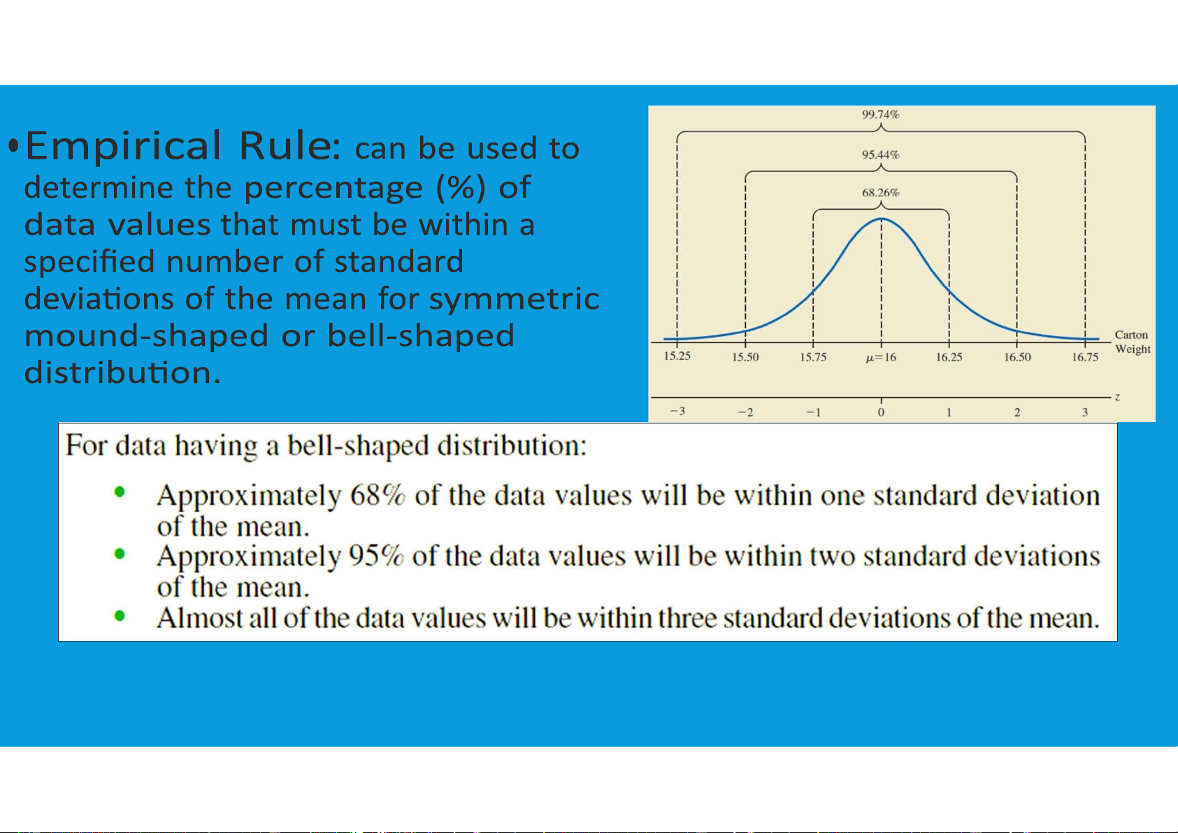
•Empirical Rule
•Detecng Outliers
3.3. MEASURES OF DISTRIBUTION SHAPE, RELATIVE LOCATION, AND DETECTING
OUTLIERS
tu@hcmiu.edu.vn 3
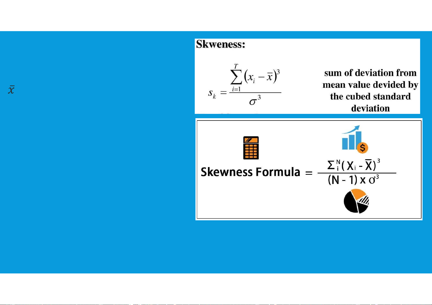
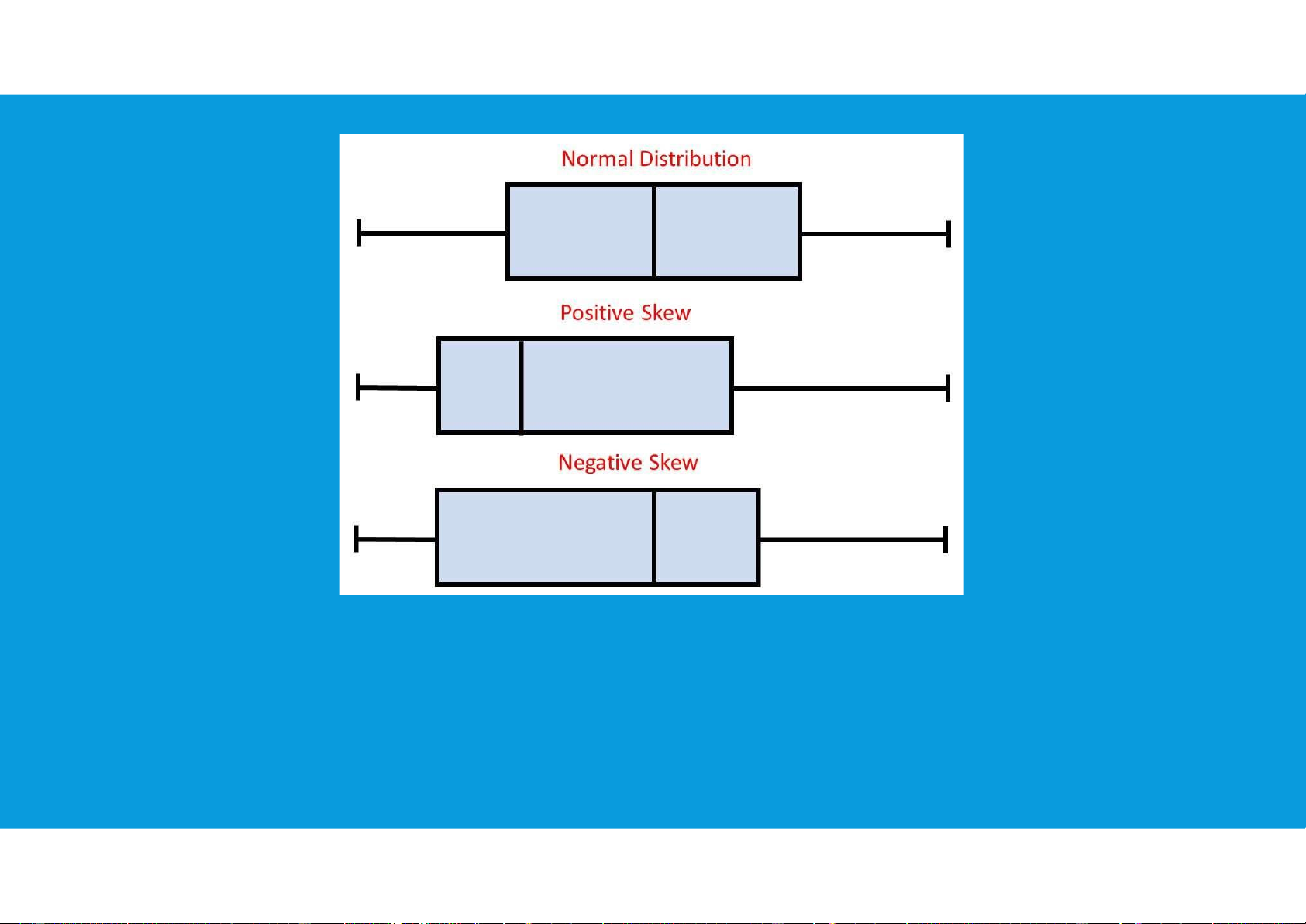
•Distribuon Shape:
•x
i
= i
th
Random Variable
= Mean of the Distribuon
•n = Number of Variables in the
Distribuon
•σ (or s) = Standard Distribuon
3.3. MEASURES OF DISTRIBUTION
SHAPE, RELATIVE LOCATION, AND
DETECTING OUTLIERS
tu@hcmiu.edu.vn 4
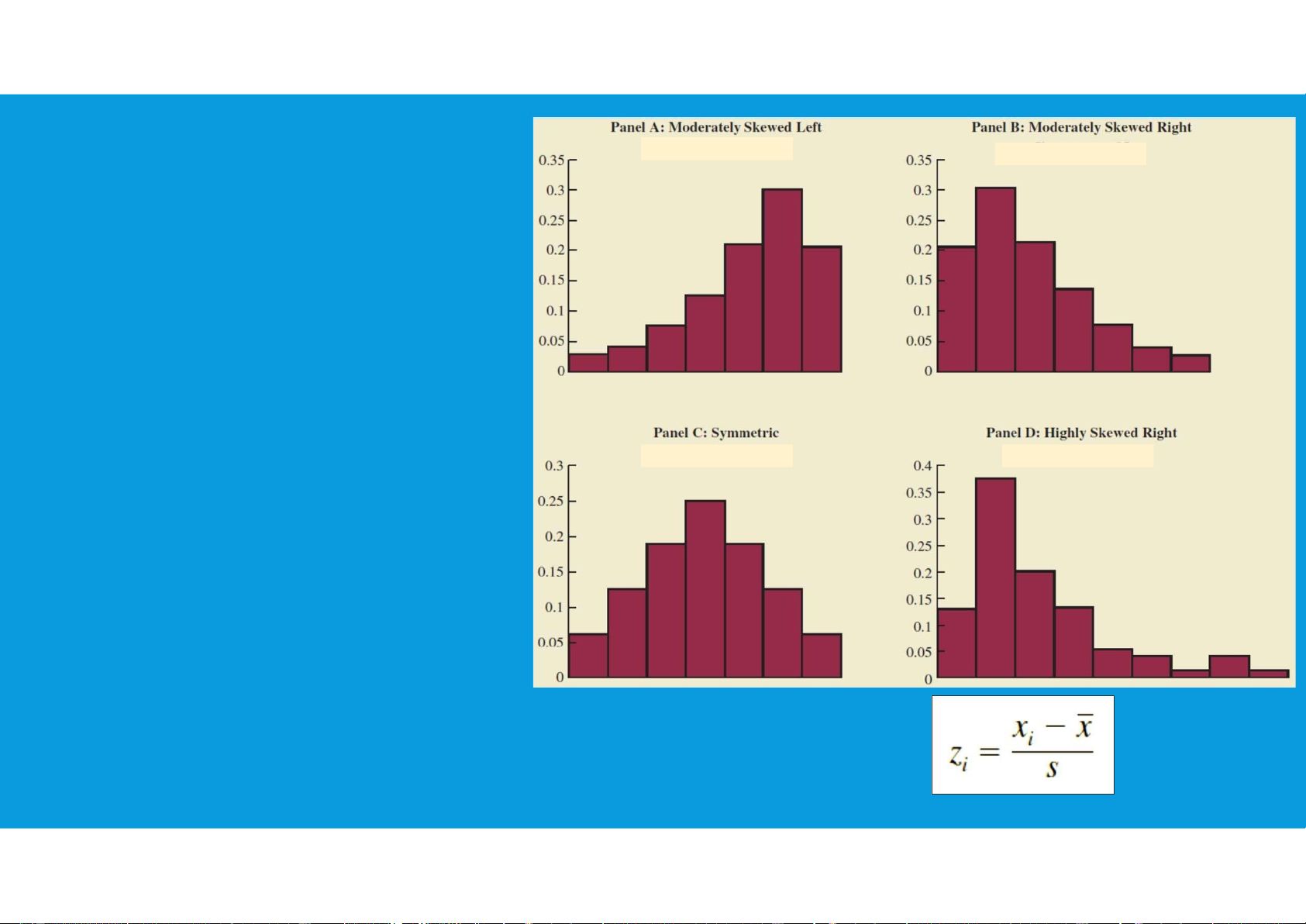
•Distribuon Shape:
•For a symmetric distribuon,
the mean and the median are
equal.
•When the data are posively
skewed, the mean will usually
be greater than the median.
•When the data are negavely
skewed, the mean will usually
be less than the median.
3.3. MEASURES OF
DISTRIBUTION SHAPE, RELATIVE
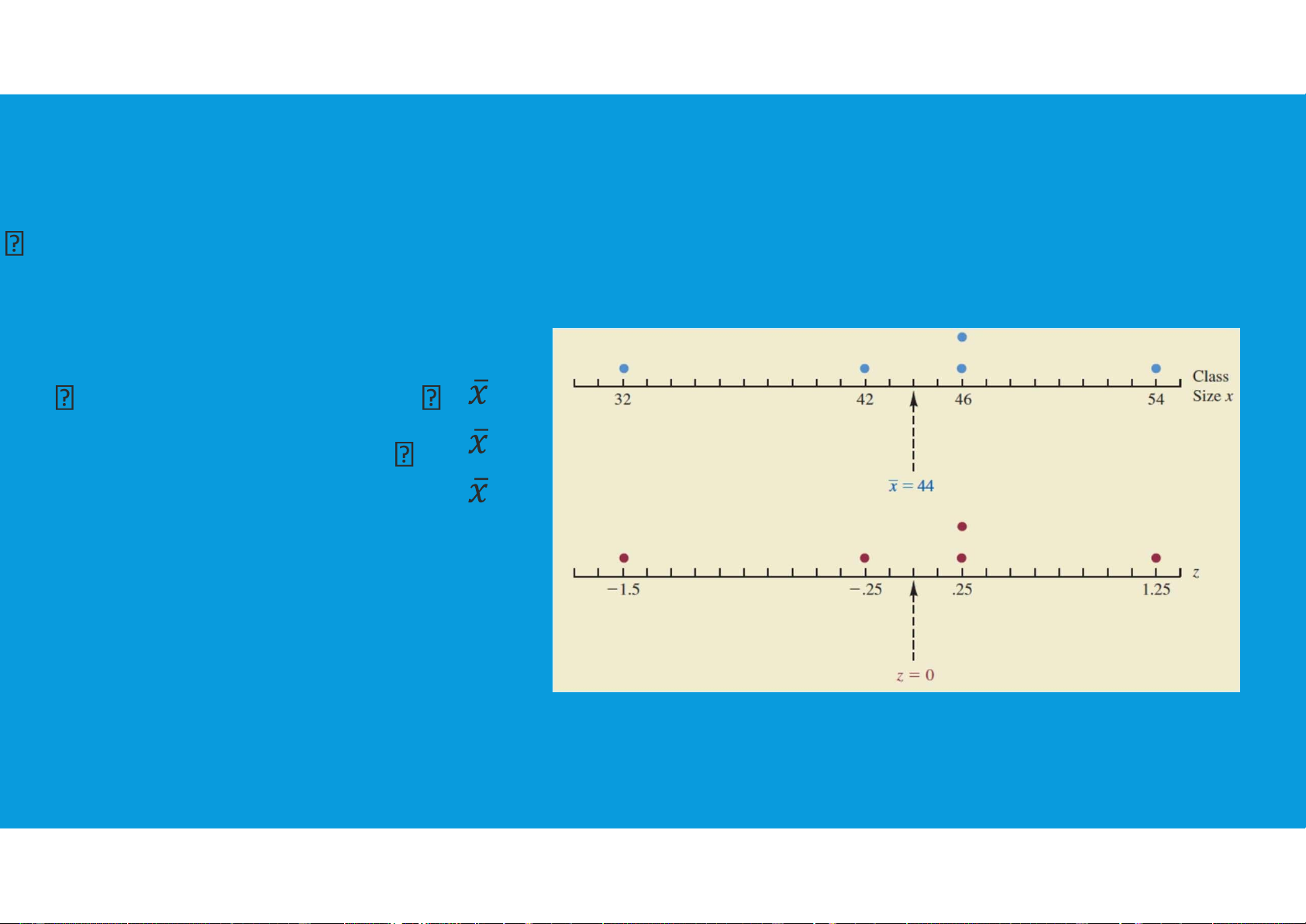
LOCATION, AND DETECTING OUTLIERS •z-Scores: By using both the
tu@hcmiu.edu.vn 5
mean and standard deviaon, we can determine the relave locaon of any
observaon i.
The z-score is oen called the standardized value.
•The z-score, z
i
, can be interpreted as the number of standard deviaons x
i
is from
the mean x.
z-score > 0 means x
i
>
z-score < 0 means x
i
< z-
score = 0 means x
i
=
3.3. MEASURES OF
DISTRIBUTION SHAPE,
RELATIVE LOCATION, AND
DETECTING OUTLIERS
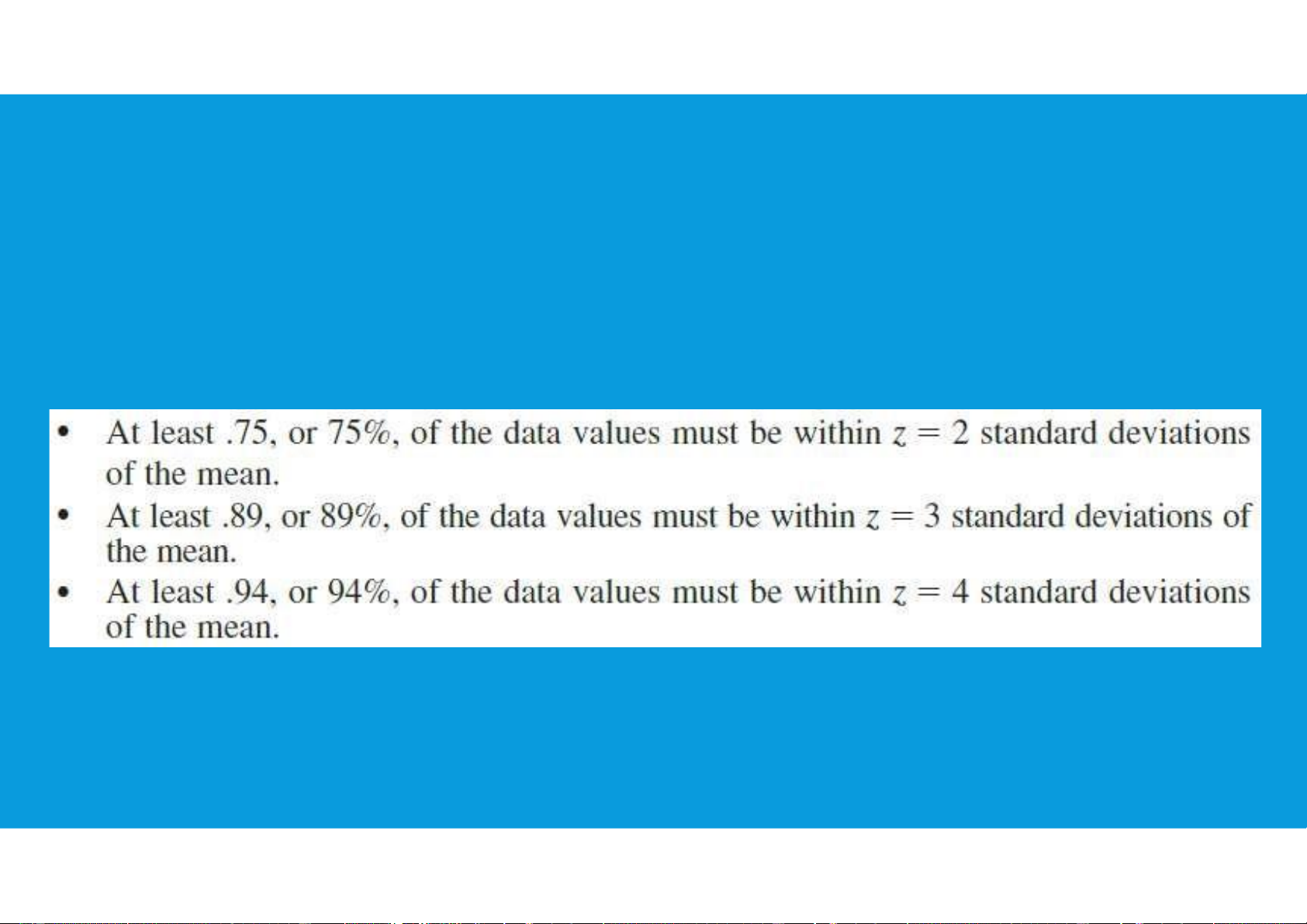
•Chebyshevs Theorem: enables us to make statements about the
tu@hcmiu.edu.vn 6
proporon (%) of data values that must be within a specied number of standard
deviaons of the mean (applied for all distribuon shapes).
At least (1 − 1/z
2
) of the data values must be within z standard deviaons of the
mean, where z is any value greater than 1.
(but z need not be an integer)
3.3. MEASURES OF DISTRIBUTION SHAPE, RELATIVE LOCATION, AND
DETECTING OUTLIERS
tu@hcmiu.edu.vn 7
3.3. MEASURES OF DISTRIBUTION SHAPE, RELATIVE LOCATION, AND DETECTING
OUTLIERS
tu@hcmiu.edu.vn 8
•Detecng Outliers:
•Somemes a data set will have one or more observaons with unusually large or
unusually small values. These extreme values are called outliers.
•An outlier may be a data value that has been incorrectly recorded that needed to
be corrected or removed before further analysis.
- Standardized values (z-scores) can be used to idenfy outliers
Treat any data value with a z-score less than −3 or greater than +3 as an outlier
3.3. MEASURES OF DISTRIBUTION SHAPE, RELATIVE LOCATION, AND DETECTING
OUTLIERS
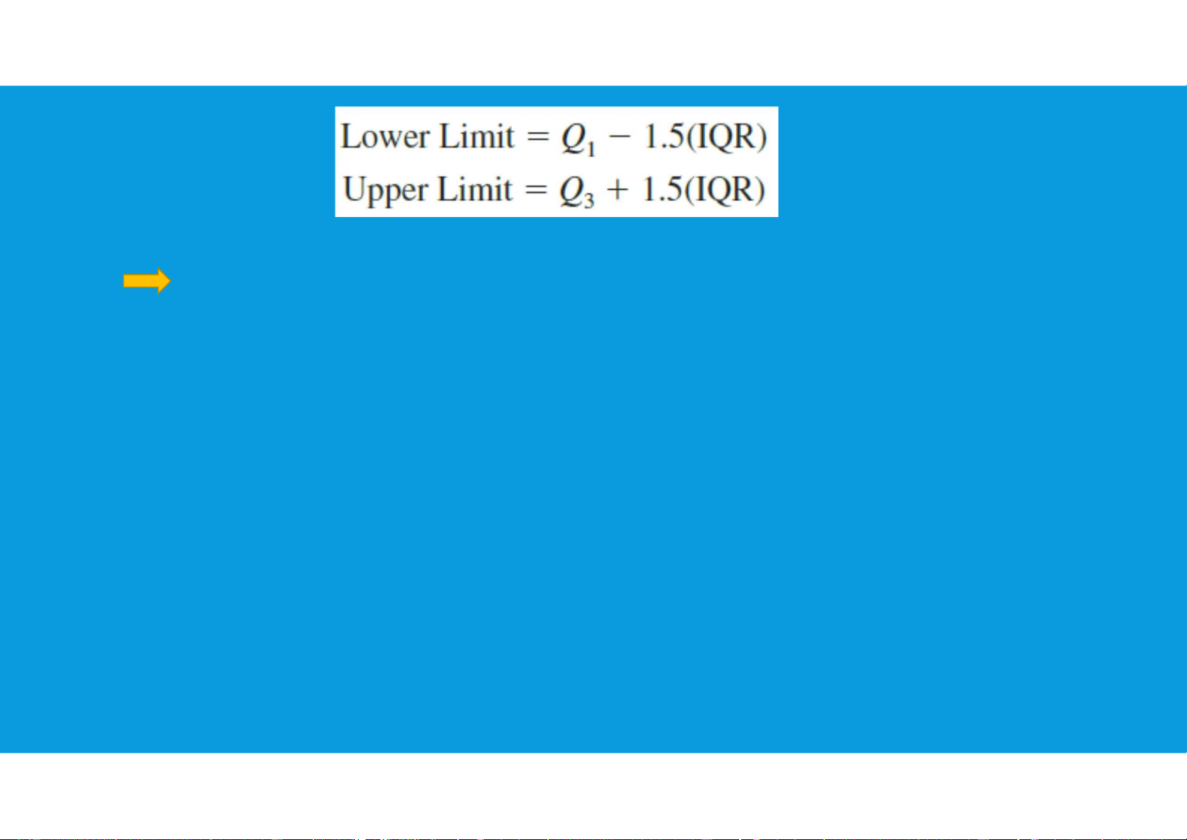
•Detecng Outliers:
- Another approach to idenfying outliers is based upon the values of the rst and
third quarles (Q
1
and Q
3
) and the interquarle range (IQR).
tu@hcmiu.edu.vn 9
An observaon is classied as an outlier if its value is less than
the lower limit or greater than the upper limit
lOMoARcPSD|47231818
End of le 1.
Any quesons?
tu@hcmiu.edu.vn
10
3.4. FIVE NUMBERS SUMMARIES AND BOX PLOTS
•Five-Number Summary
•Box Plot
•Comparave Analysis Using Box Plots
lOMoARcPSD|47231818
tu@hcmiu.edu.vn 11
3.4. FIVE NUMBERS SUMMARIES AND BOX PLOTS
•Five-Number Summary: is especially useful in descripve analyses or during
the preliminary invesgaon of a large data set.
A summary consists of ve values: the most extreme values in the data set (the
maximum and minimum values), the lower and upper quarles, and the median.
lOMoARcPSD|47231818
tu@hcmiu.edu.vn 12
3.4. FIVE NUMBERS SUMMARIES AND BOX PLOTS
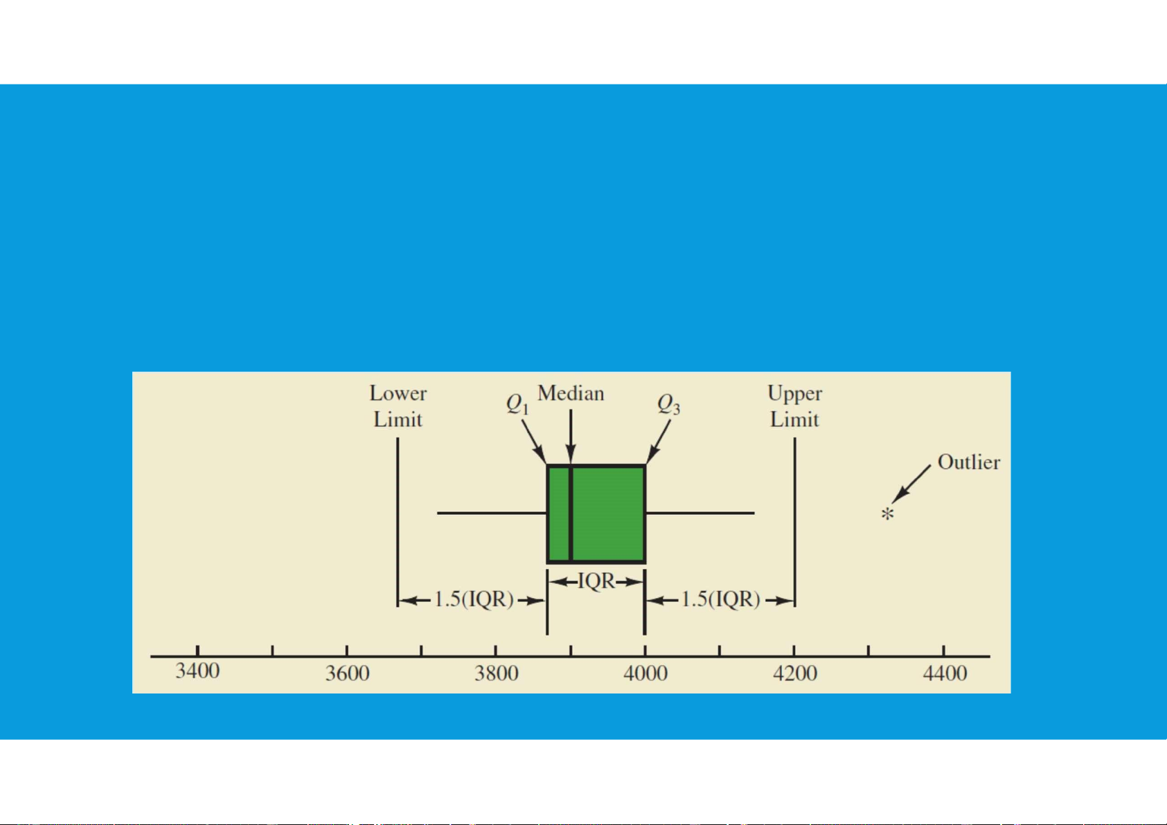
•Box Plot: A box plot is a graphical display of data based on a venumber
summary. A key to the development of a box plot is the computaon of the
interquarle range, IQR = Q
3
− Q
1
.
lOMoARcPSD|47231818
tu@hcmiu.edu.vn 13
lOMoARcPSD|47231818
tu@hcmiu.edu.vn 14
3.4. FIVE NUMBERS SUMMARIES AND BOX PLOTS
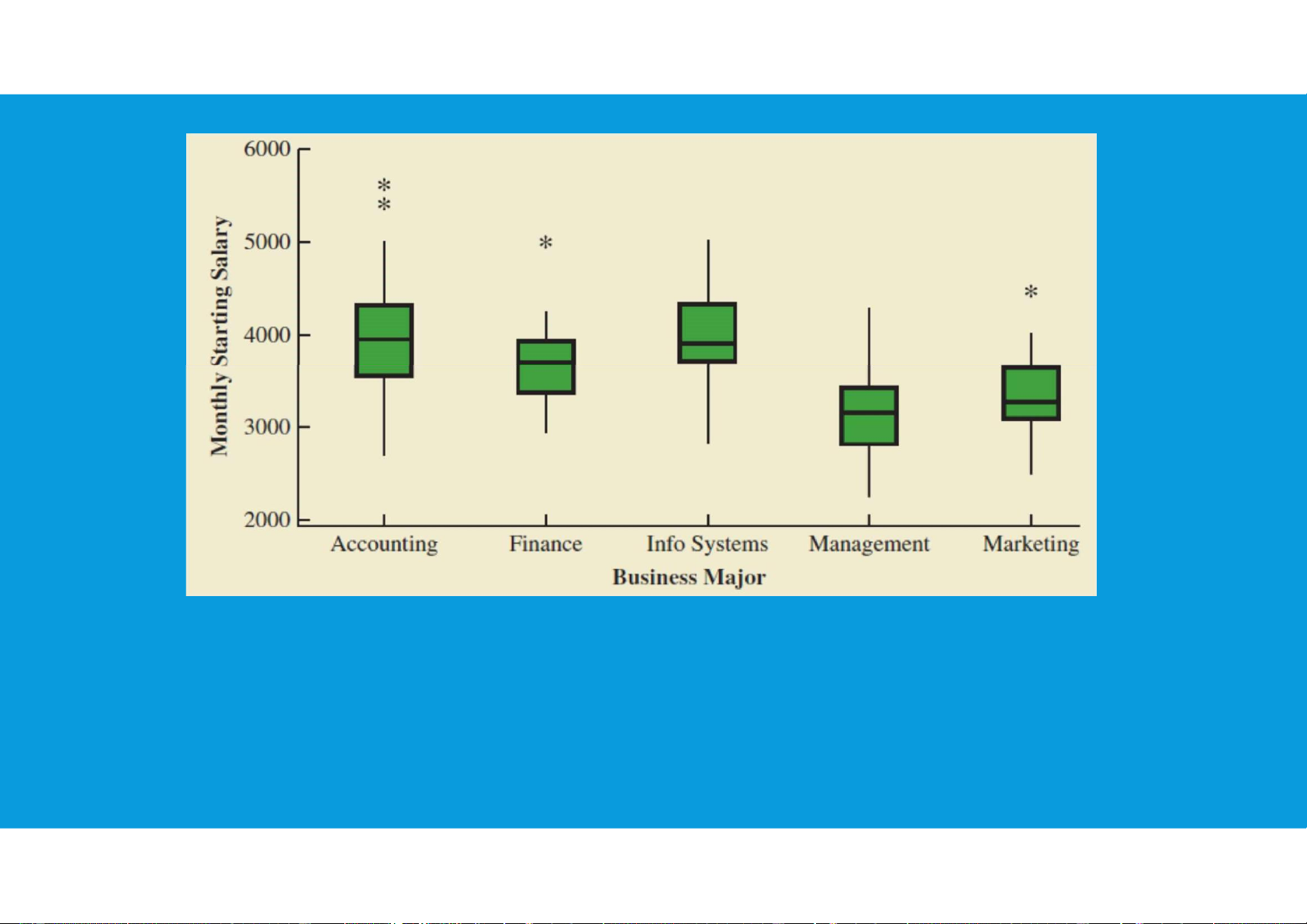
•Comparave Analysis Using Box Plots: Box plots can also be used to
provide a graphical summary of two or more groups and facilitate visual
comparisons among the groups.
lOMoARcPSD|47231818
tu@hcmiu.edu.vn 15
lOMoARcPSD|47231818
End of le 2.
Any quesons?
tu@hcmiu.edu.vn
15
3.5. MEASURES OF ASSOCIATION BETWEEN TWO VARIABLES
•Covariance
•Interpretaon of the Covariance
•Correlaon Coecient
lOMoARcPSD|47231818
tu@hcmiu.edu.vn 17
•Interpretaon of the Correlaon Coecient
3.5. MEASURES OF ASSOCIATION BETWEEN TWO VARIABLES
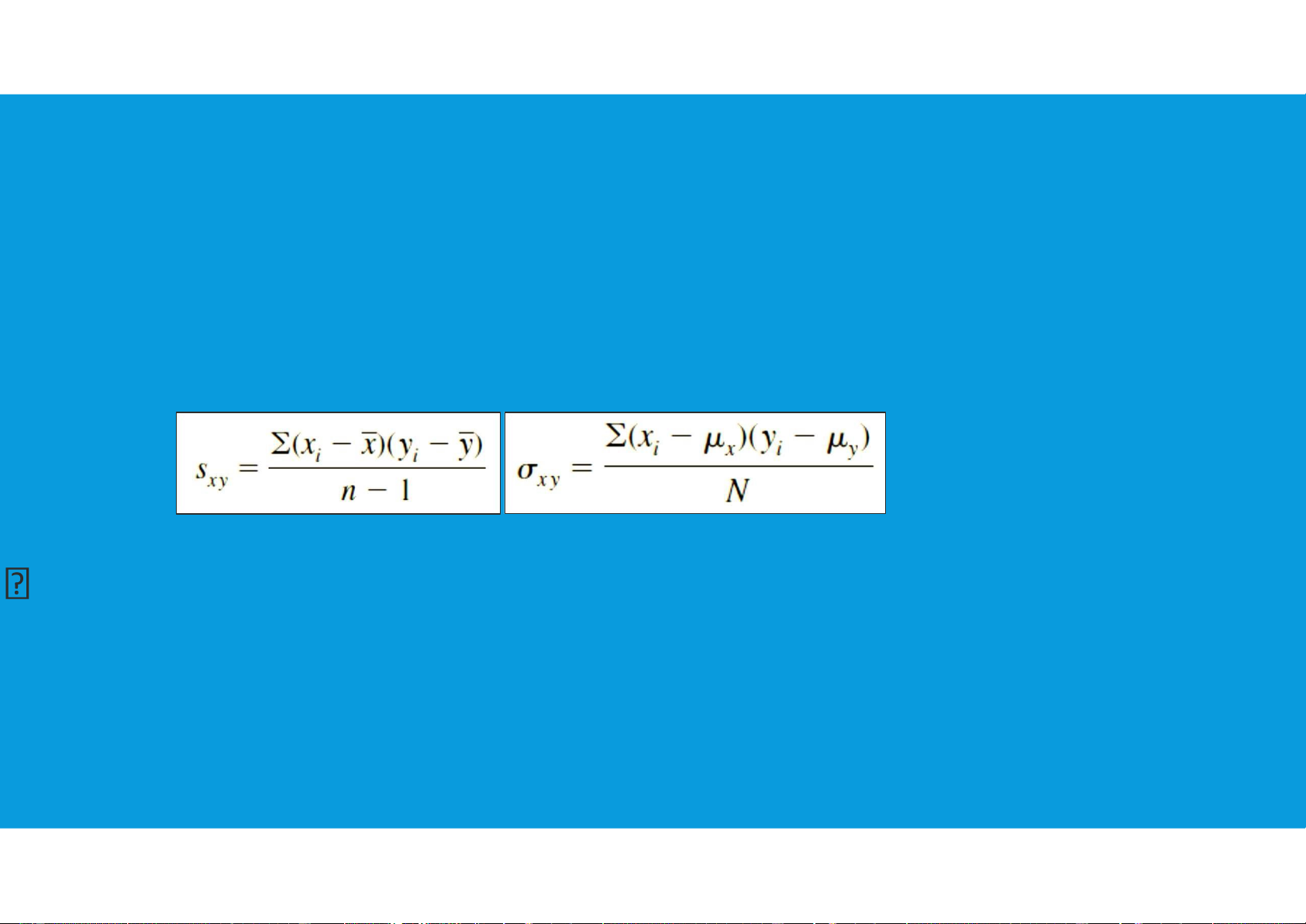
•Covariance: For a sample of size n with the observaons (x
1
, y
1
),
(x
2
, y
2
), and so on, the sample covariance and populaon covariance are dened
as follows:
To measure the strength of the linear relaonship between x and y
lOMoARcPSD|47231818
tu@hcmiu.edu.vn 18
3.5. MEASURES OF ASSOCIATION BETWEEN TWO VARIABLES
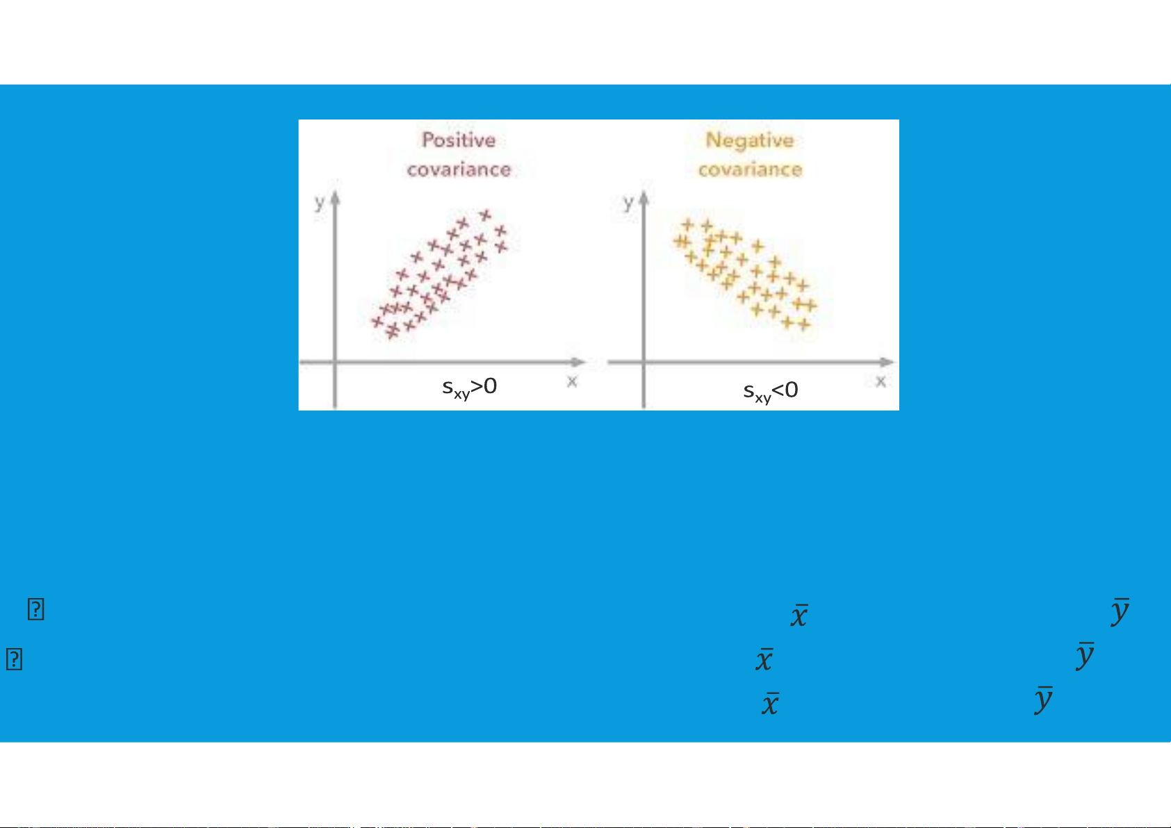
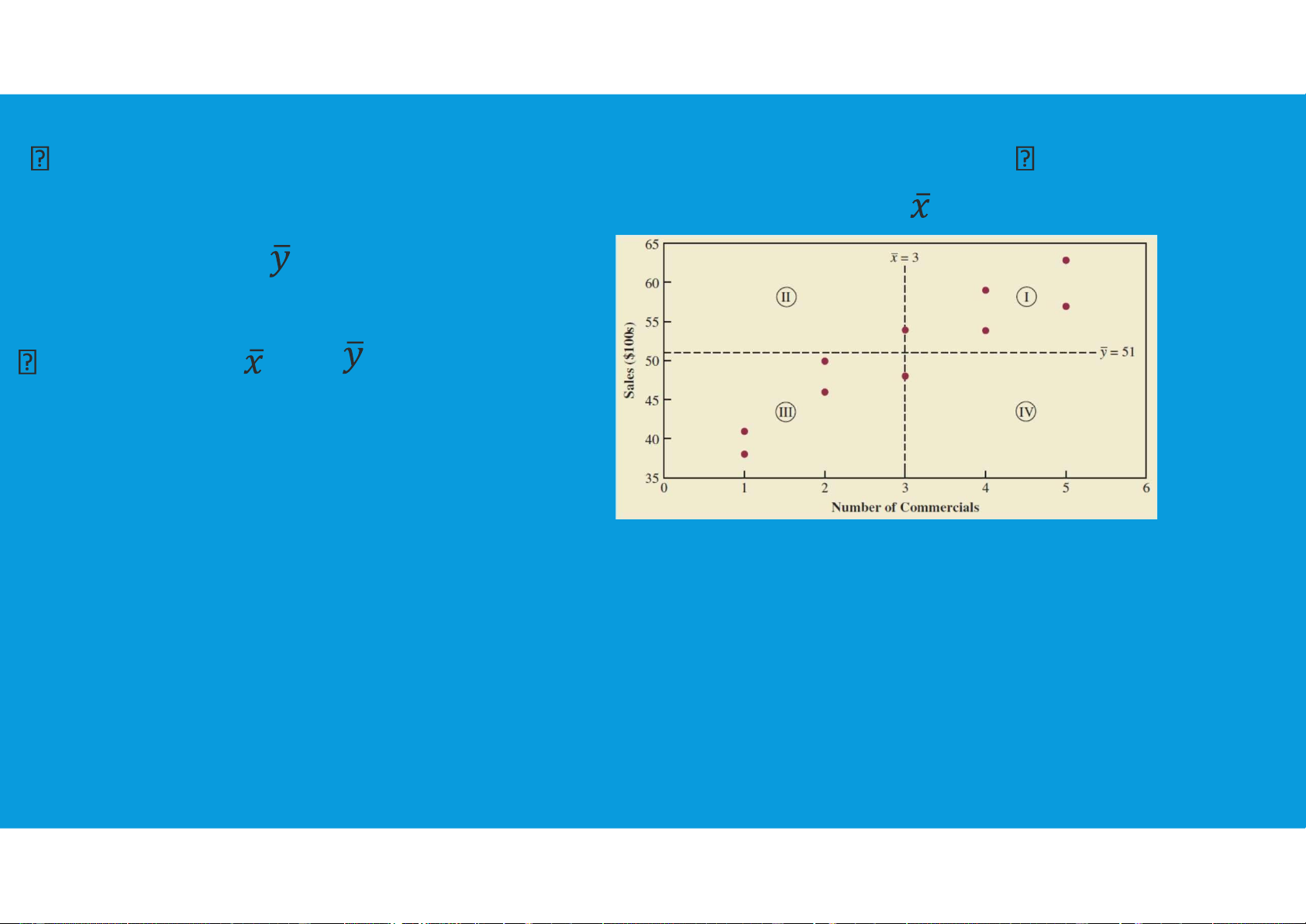
•Interpretaon of the Covariance: The lines divide the graph into four
quadrants:
Points in quadrant I correspond to x
i
greater than and y
i
greater than
Points in quadrant II correspond to x
i
less than and y
i
greater than
lOMoARcPSD|47231818
tu@hcmiu.edu.vn 19
Points in quadrant III correspond to x
i
less than and y
i
less than Points in
quadrant IV correspond to x greater than
and y less than
value of (x
i
)(y
i
) must be:
- posive for points in quadrant I
- negave for points in quadrant II
- posive for points in quadrant III
- negave for points in quadrant IV
3.5. MEASURES OF ASSOCIATION BETWEEN TWO VARIABLES
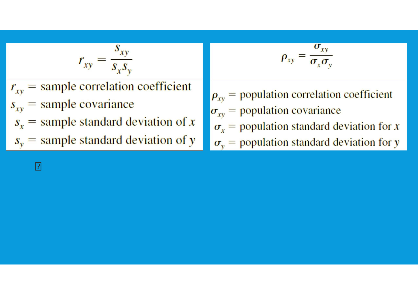
•Correlaon Coecient: Person product moment correlaon coecient:
lOMoARcPSD|47231818
tu@hcmiu.edu.vn 20
the sample correlaon coecient r
xy
is a point esmator of the
populaon correlaon coecient ρ
xy
.
3.5. MEASURES OF ASSOCIATION BETWEEN TWO VARIABLES
•Interpretaon of the Correlaon Coecient:
| 1/22

Preview text:

APPLIED STATISTICS COURSE CODE: ENEE1006IU Lecture 5:
Chapter 3: Descriptive statistics
(3 credits: 2 is for lecture, 1 is for lab-work)
Instructor: TRAN THANH TU Email: tttu@hcmiu.edu.vn tttu@hcmiu.edu.vn 1
3.3. MEASURES OF DISTRIBUTION SHAPE, RELATIVE LOCATION, AND DETECTING OUTLIERS •Distribution Shape •z-Scores •Chebyshev’s Theorem •Empirical Rule •Detecting Outliers
3.3. MEASURES OF DISTRIBUTION SHAPE, RELATIVE LOCATION, AND DETECTING OUTLIERS tttu@hcmiu.edu.vn 2 •Distribution Shape: •xi = ith Random Variable
• = Mean of the Distribution
•n = Number of Variables in the Distribution
•σ (or s) = Standard Distribution 3.3. MEASURES OF DISTRIBUTION SHAPE, RELATIVE LOCATION, AND DETECTING OUTLIERS tttu@hcmiu.edu.vn 3 •Distribution Shape:
•For a symmetric distribution, the mean and the median are equal.
•When the data are positively skewed, the mean will usually be greater than the median.
•When the data are negatively skewed, the mean will usually be less than the median. 3.3. MEASURES OF DISTRIBUTION SHAPE, RELATIVE
LOCATION, AND DETECTING OUTLIERS •z-Scores: By using both the tttu@hcmiu.edu.vn 4
mean and standard deviation, we can determine the relative location of any observation i.
The z-score is often called the standardized value.
•The z-score, zi, can be interpreted as the number of standard deviations xi is from the mean x. z-score > 0 means xi >
z-score < 0 means xi < z- score = 0 means xi = 3.3. MEASURES OF DISTRIBUTION SHAPE, RELATIVE LOCATION, AND DETECTING OUTLIERS
•Chebyshev’s Theorem: enables us to make statements about the tttu@hcmiu.edu.vn 5
proportion (%) of data values that must be within a specified number of standard
deviations of the mean (applied for all distribution shapes).
“At least (1 − 1/z2) of the data values must be within z standard deviations of the
mean, where z is any value greater than 1.”
(but z need not be an integer)
3.3. MEASURES OF DISTRIBUTION SHAPE, RELATIVE LOCATION, AND DETECTING OUTLIERS tttu@hcmiu.edu.vn 6
3.3. MEASURES OF DISTRIBUTION SHAPE, RELATIVE LOCATION, AND DETECTING OUTLIERS tttu@hcmiu.edu.vn 7 •Detecting Outliers:
•Sometimes a data set will have one or more observations with unusually large or
unusually small values. These extreme values are called outliers.
•An outlier may be a data value that has been incorrectly recorded that needed to
be corrected or removed before further analysis.
- Standardized values (z-scores) can be used to identify outliers
Treat any data value with a z-score less than −3 or greater than +3 as an outlier
3.3. MEASURES OF DISTRIBUTION SHAPE, RELATIVE LOCATION, AND DETECTING OUTLIERS •Detecting Outliers:
- Another approach to identifying outliers is based upon the values of the first and
third quartiles (Q1 and Q3) and the interquartile range (IQR). tttu@hcmiu.edu.vn 8
An observation is classified as an outlier if its value is less than
the lower limit or greater than the upper limit tttu@hcmiu.edu.vn 9 lOMoARcPSD|47231818 End of file 1. Any questions? tttu@hcmiu.edu.vn 10
3.4. FIVE NUMBERS SUMMARIES AND BOX PLOTS •Five-Number Summary •Box Plot
•Comparative Analysis Using Box Plots lOMoARcPSD|47231818
3.4. FIVE NUMBERS SUMMARIES AND BOX PLOTS
•Five-Number Summary: is especially useful in descriptive analyses or during
the preliminary investigation of a large data set.
A summary consists of five values: the most extreme values in the data set (the
maximum and minimum values), the lower and upper quartiles, and the median. tttu@hcmiu.edu.vn 11 lOMoARcPSD|47231818
3.4. FIVE NUMBERS SUMMARIES AND BOX PLOTS
•Box Plot: A box plot is a graphical display of data based on a fivenumber
summary. A key to the development of a box plot is the computation of the
interquartile range, IQR = Q3 − Q1. tttu@hcmiu.edu.vn 12 lOMoARcPSD|47231818 tttu@hcmiu.edu.vn 13 lOMoARcPSD|47231818
3.4. FIVE NUMBERS SUMMARIES AND BOX PLOTS
•Comparative Analysis Using Box Plots: Box plots can also be used to
provide a graphical summary of two or more groups and facilitate visual comparisons among the groups. tttu@hcmiu.edu.vn 14 lOMoARcPSD|47231818 tttu@hcmiu.edu.vn 15 lOMoARcPSD|47231818 End of file 2. Any questions? tttu@hcmiu.edu.vn 15
3.5. MEASURES OF ASSOCIATION BETWEEN TWO VARIABLES •Covariance
•Interpretation of the Covariance •Correlation Coefficient lOMoARcPSD|47231818
•Interpretation of the Correlation Coefficient
3.5. MEASURES OF ASSOCIATION BETWEEN TWO VARIABLES
•Covariance: For a sample of size n with the observations (x1, y1),
(x2, y2), and so on, the sample covariance and population covariance are defined as follows:
To measure the strength of the linear relationship between x and y tttu@hcmiu.edu.vn 17 lOMoARcPSD|47231818
3.5. MEASURES OF ASSOCIATION BETWEEN TWO VARIABLES
•Interpretation of the Covariance: The lines divide the graph into four quadrants:
Points in quadrant I correspond to xi greater than and yi greater than
Points in quadrant II correspond to xi less than and yi greater than tttu@hcmiu.edu.vn 18 lOMoARcPSD|47231818
Points in quadrant III correspond to xi less than and yi less than Points in
quadrant IV correspond to x greater i i than and y less than
value of (xi − )(yi − ) must be:
- positive for points in quadrant I
- negative for points in quadrant II
- positive for points in quadrant III
- negative for points in quadrant IV
3.5. MEASURES OF ASSOCIATION BETWEEN TWO VARIABLES
•Correlation Coefficient: Person product moment correlation coefficient: tttu@hcmiu.edu.vn 19 lOMoARcPSD|47231818
the sample correlation coefficient rxy is a point estimator of the
population correlation coefficient ρxy.
3.5. MEASURES OF ASSOCIATION BETWEEN TWO VARIABLES
•Interpretation of the Correlation Coefficient: tttu@hcmiu.edu.vn 20