Distributed Fuzzy Clustering & Routing for WSNs | Iot và ứng dụng | Học viện Công nghệ Bưu chính Viễn thông
Due to inherent issue of energy limitation in sensor nodes, the energy conservation is the primary concern for large-scale wireless sensor networks. Cluster-based routing has been found to be an effective mechanism to reduce the energy consumption of sensor nodes. In clustered wireless sensor networks, the network is divided into a set of clusters; each cluster has a coordinator, called cluster head (CH). Each node of a cluster transmits its collected infor- mation to its CH that in turn aggregates the received information and sends it to the base station directly or via other CHs. In multihop communication. Tài liệu được sưu tầm và soạn thảo dưới dạng file PDF để gửi tới các bạn cùng tham khảo, ôn tập đầy đủ kiến thức, chuẩn bị cho các buổi học thật tốt. Mời bạn đọc đón xem!
Môn: IoT và ứng dụng 143 tài liệu
Trường: Học viện Công Nghệ Bưu Chính Viễn Thông 1.8 K tài liệu
Tác giả:


Preview text:
Received: 4 June 2017 Revised: 22 November 2017 Accepted: 15 April 2018 DOI: 10.1002/dac.3709
R E S E A R C H A R T I C L E
Distributed fuzzy approach to unequal clustering and
routing algorithm for wireless sensor networks Nabajyoti Mazumdar Hari Om
Department of Computer Science and
Engineering, Indian Institute of Summary
Technology (ISM), Dhanbad, India
Due to inherent issue of energy limitation in sensor nodes, the energy con- Correspondence
servation is the primary concern for large-scale wireless sensor networks.
Nabajyoti Mazumdar, Indian Institute of
Cluster-based routing has been found to be an effective mechanism to reduce
Technology (ISM), Dhanbad, India.
the energy consumption of sensor nodes. In clustered wireless sensor networks, Email: nabajyoti@cse.ism.ac.in
the network is divided into a set of clusters; each cluster has a coordinator,
called cluster head (CH). Each node of a cluster transmits its collected infor-
mation to its CH that in turn aggregates the received information and sends it
to the base station directly or via other CHs. In multihop communication, the
CHs closer to the base station are burdened with high relay load; as a result,
their energy depletes much faster as compared with other CHs. This problem
is termed as the hot spot problem. In this paper, a distributed fuzzy logic-based
unequal clustering approach and routing algorithm (DFCR) is proposed to solve
this problem. Based on the cluster design, a multihop routing algorithm is also
proposed, which is both energy efficient and energy balancing. The simula-
tion results reinforce the efficiency of the proposed DFCR algorithm over the
state-of-the-art algorithms, ie, energy-aware fuzzy approach to unequal cluster-
ing, energy-aware distributed clustering, and energy-aware routing algorithm,
in terms of different performance parameters like energy efficiency and network lifetime. KEYWORDS
clustering, hot spot, network lifetime, routing, wireless sensor networks 1 INTRODUCTION
The developments of micro–electrical-mechanical systems, digital systems, and wireless communication technologies
have enabled the miniaturized wireless sensors. A sensor node can sense a limited area for a given activity. To collect infor-
mation over a large area, the data should be collected through the cooperative functioning of a set of sensor nodes. These
cooperatively functioning sensors form a wireless sensor network (WSN). The WSNs have gained enormous attention
due to their usage in different applications like disaster management, home, and health applications.1,2 A WSN consists
of a large number of tiny sensor nodes, which are deployed randomly or deterministically to monitor a given target area.
The sensor nodes are generally equipped with low powered battery that cannot be replaced or recharged once deployed.
Thus, the sensor nodes' energy needs to be efficiently used to have longer life of the network. Further, considering differ-
ent constraints of WSNs, an algorithm designed for WSNs must have the following characteristics: (1) distributed nature,
Int J Commun Syst. 2018;e3709.
wileyonlinelibrary.com/journal/dac
Copyright © 2018 John Wiley & Sons, Ltd. 1 of 23
https://doi.org/10.1002/dac.3709 2 of 23 MAZUMDAR AND OM
(2) minimize energy consumption, and (3) efficient time and message complexity. Clustering has been found to be an
efficient approach to conserve the energy of a sensor node. In clustered WSNs, the sensor nodes are organized into clus-
ters; each cluster has a coordinator, called cluster head (CH), and set of members, called cluster members (CMs).2 All
CMs sense the environment and send their sensed data to their respective CHs. The CHs aggregate the received data to
remove the redundancy and then forward it to the base station (BS). Many centralized and distributed clustering algo-
rithms have been discussed in literature.3-20 For a large-scale WSN, the centralized algorithms are somewhat ineffective,
as they require the entire network information to be available at the BS. On the other hand, in distributed approach, a sen-
sor takes the necessary decision (like CH selection and data routing) based on only its local information. The clustering
in a WSN has the following advantages:
1. Reduction in energy consumption: It reduces the energy consumption in a WSN as only the CH of each cluster is involved
in data aggregation and routing.
2. Ease of management: Routing can easily be managed as only the CHs participate in the routing process. Hence, it
improves the scalability of WSNs.
3. Preservation of communication bandwidth: It conserves significant communication bandwidth as, in a cluster, the CMs
send their data to their respective CHs only and the CHs aggregate the received data, thus significantly reducing the
amount of data to be sent to the BS.
In clustered WSNs, the CHs are burdened with additional responsibilities like collecting the data from their CMs,
aggregating it, and communicating it to the BS. This leads to depletion of their energy much faster as compared with
the non-CH nodes. To overcome this problem, the CH rotation mechanism has been adopted by most of the clustering
algorithms, where the responsibility of a CH is uniformly distributed among the sensor nodes in network. For CH-BS
communication, either single-hop or multihop communication models are used. In single-hop communication, the CHs
communicate directly to the BS. Since such long haul communication is very energy demanding, it may not be feasible
for large-scale WSNs, whereas the multihop communication is found to be an efficient approach to prolong the network
lifetime in WSNs.21-35 Here, the CHs send their data via other CHs to reach the BS. However, in this situation, the CHs
near the BS are burdened with heavy data traffic load, as they are required to forward all incoming packets, which conse-
quences in the premature energy depletion of such CHs. This problem is termed as energy hole or hot spot problem. To
avoid such problem, some unequal clustering algorithms have been discussed in recent years.8,36-43 In these algorithms,
the cluster size closer to the BS is kept smaller as compared with the clusters away from the BS. This ensures availability
of more CHs closer to the BS to share the high data traffic load.
In this paper, an energy-aware distributed cluster-based routing algorithm is proposed to enhance the network lifetime
in WSNs. The clustering algorithm forms the clusters of unequal sizes, where the cluster radius is calculated using a
distributed fuzzy logic approach. The unequal clustering helps to avoid the hot spot problem. The CHs are selected based
on the remaining energy of the nodes and their distance from the BS. For CH to BS communication, a virtual network
of CHs is constructed, where CHs route their data towards the BS via other CHs. The routing path is formed based on
a cost function. We have performed experiments for the proposed algorithm DFCR to evaluate its efficacy in terms of
energy consumption and network lifetime over the existing algorithms, namely, energy-aware fuzzy approach to unequal
clustering (EAUCF),36 energy-aware distributed clustering (EADC),29 and energy-aware routing algorithm (ERA).33
The remaining part of the paper is organized as follows. Section 2 provides a survey of the related work, and Section
3 describes the system model and terminologies used in the paper. The proposed clustering and routing algorithms are
presented in Section 4. The complexity analyses of the proposed algorithms are given in Section 5. In Section 6, the
simulation results are presented, and finally, the paper is concluded in Section 7. 2 RELATED WORK
There have been discussed many clustering algorithms3-20 and routing techniques21-32 in recent years for WSNs. They
mainly aim to reduce the energy depletion of the sensor nodes in order to maximize the lifetime of the network. The
LEACH4 is a well-known clustering algorithm for WSNs in which the sensor nodes are selected as CHs based on some
probability. Although the LEACH algorithm enhances the network lifetime, yet it cannot guarantee that the selected CHs
are evenly placed in the network. Further, in this algorithm, some low energy sensor nodes may be selected as the CHs;
as a result, their energy will deplete quickly, thus creating the energy holes in the network. To overcome this drawback,
many variants of LEACH have been discussed that include PEGASIS,9 TEEN,7 and HEED protocol.5 Most of the clustering MAZUMDAR AND OM 3 of 23
algorithms elect the CHs based on a single parameter like residual energy, node degree, and distance from neighbors.
Since the efficiency of clustering depends on multiple parameters, the strategies considering multiple parameters are
highly desired. Many researchers have used fuzzy logic to deal with such concerns in WSNs. Previous work16 discusses
a fuzzy-based CH election method by considering the residual energy, node centrality, and node degree as fuzzy input
parameters. This algorithm provides significant improvement in network lifetime; however, being a centralized algorithm,
it is not suitable for large-scale WSNs. Previous study17 introduces a distributed fuzzy logic approach, called CHEF, for
clustering in WSNs. In this method, initially, a set of tentative CHs are selected based on a probabilistic approach like
that in LEACH and then these tentative CHs compute their chance to be final CHs using a fuzzy logic method with input
variables as residual energy and local distance. Here, the local distance is sum of distances of a node from its neighbors.
Although the CHEF provides better lifetime, yet like LEACH due to the probabilistic election of tentative CHs, the CHs
may not be uniformly distributed in the network. This issue has been addressed in ECPF,18 where the tentative CHs are
selected based on the residual energy of nodes and the final CHs are computed using fuzzy logic by considering the node
degree and the node centrality as fuzzy input variables. The SEP-FL42 is another fuzzy logic-based clustering algorithm
that considers battery level, distance to the BS, and the density along with a threshold value for CH selection.
One major drawback of these algorithms is that the CHs communicate with the BS directly (via single-hop commu-
nication). Such long haul communication is quite energy consuming and hence not suitable for a large-scale network.
So many algorithms have been discussed considering the multihop cluster-based routing.22,23,29,31,39 Similar to the ECPF,
the EADC-FL39 selects a set of tentative CHs based on the remaining energy of the sensor nodes and the final CHs are
selected by considering the node centrality and the node degree as fuzzy input variables. Unlike the ECPF, the EADC-FL
considers multihop communication to transfer the data from CHs to BS. Here, a CH considers the residual energy and
the number of CMs of the forwarding CHs to form a routing tree. Another work22 discusses the minimum hop routing
model algorithm in which the CHs select the routing path such that the hop count to the BS is minimized. To minimize
the hop count, the CHs transmit data to a larger distance, which consumes much amount of energy. In Yu et al,23 an
energy-efficient and power-aware algorithm is discussed in which the BS receives the route request message from all CHs
via different paths, and based on these messages, the BS computes the cost of each path by using the residual energy of
the CHs in the path. The BS sends the route cost reply message using the same reverse path. In case a CH receives the
multiple routes reply messages, it chooses the path with minimum cost. Although this algorithm constructs an efficient
routing path, yet it has high cost of message exchange. The study ERA33 discusses an energy-efficient routing strategy
with constant message and time complexity where the CHs distribute the data packets to the next-hop CHs based on the
ratio of their residual energies. In Yu et al,29 the EADC algorithm is discussed in which the routing path is selected by
considering the residual energy of CHs and the average energy of its neighbors. In Javaherian and Haghighat,31 the fuzzy
clustering and minimum cost tree algorithm is discussed by considering the distance to the BS and the residual energy to
select the CH. Each CH selects the closest forwarding CH to transmit its data to the BS that results in selecting the same
routing path by the CHs, which will lead to early depletion of energy for these forwarding CHs.
None of these algorithms have considered the hot spot problem, which leads to network partitioning. In energy-efficient
unequal clustering8 and distributed energy and coverage-aware routing,43 the clusters are formed with unequal sizes to
encounter the hot spot problem. Here, the size of a cluster nearer to the BS is smaller as compared with those which are
away from the BS. Although this algorithm adopts unequal clustering approach to avoid the hot spot problem, yet the
cluster size of a CH does not adapt to the change in the residual energy of sensor nodes dynamically. So the cluster radius
of a CH remains the same, no matter how much energy remains in it. The fuzzy logic-based approaches have been found
to be very effective for unequal clustering36-42,44 since it is capable of sensibly blending several parameters. The researchers
have used fuzzy logic in a distributed manner to compute the cluster radius for CHs. In Bagci and Yazici,36 an EAUCF
is discussed in which the CHs are selected using a probabilistic approach similar to the LEACH and the cluster radius
is calculated by using the CH's residual energy and its distance from the BS as fuzzy inputs. The probabilistic approach
for CH selection in EAUCF might result in electing some low energy nodes as CHs, and also, it does not consider any
parameter to deal with intracluster communication cost. The MOFCA40 and FBUC44 are modified versions of EAUCF,
where the MOFCA considers node density and the FBUC considers node degree parameter along with the residual energy
and distance to the BS for cluster radius computation. Similar to EAUCF, a common drawback in both MOFCA and FBUC
is the randomized selection of tentative CHs. The DUCF41 uses a non-probabilistic approach for CH selection where
the residual energy, node degree, and distance to BS are the considered fuzzy input parameters for both CH selection
and cluster radius computation. The fuzzy-based unequal clustering (UCF)37 is another fuzzy-based unequal clustering
approach for WSNs in which a nonprobabilistic approach is used for CH selection by considering the residual energy of a
node. For cluster radius computation, the distance to BS and the node density are taken as the fuzzy input parameters. In 4 of 23 MAZUMDAR AND OM
the EAUCF, MOFCA, DUCF, and UCF, after the CH selection, a non-CH node joins the closest CH within its proximity,
which may result in nonuniform load distribution among the clusters. In spite of the above-mentioned shortcomings,
all the fuzzy-based unequal clustering algorithms (EAUCF, MOFCA, FBUC, DUCF, and UCF) have shown significant
improvement over the traditional equal and unequal clustering methods to deal with the hot spot problem.
In the proposed DFCR algorithm, a fuzzy logic-based unequal clustering approach has been proposed to address the
hot spot problem during routing phase that has the following advantages:
1. CH selection: Sensor nodes having higher energy and closer to the BS are given higher priority to be selected as CHs.
Here, the energy parameter ensures that the energy-rich nodes perform the functionality of a CH, whereas the distance
from the BS parameter ensures the availability of more CHs closer to the BS to share the high data forwarding load.
2. Adaptive unequal clustering: The CHs dynamically adapt their cluster radii based on their current status. This means
that the radius of a CH changes as its remaining energy reduces. Hence, significant amount of energy can be conserved.
3. Routing: To balance the energy consumption, the CHs transmit the data to the next-hop CH, which corresponds to the minimum cost value.
4. Distributed nature: During clustering and routing, the sensor nodes require only the local information to take necessary
decisions; hence, it is completely distributed. 3
SYSTEM MODEL AND TERMINOLOGIES
Here, we present the network model assumed in this work along with the energy model and terminologies used in it. 3.1 Network model
We make the following assumptions for the underlying network:
1. A set of homogeneous sensor nodes deployed randomly over a given target area.
2. Nodes are stationary after deployment.
3. A sensor node can join only one CH within its communicating range.
4. BS has no energy constraint.
5. Wireless link is symmetric and bidirectional. 3.2 Energy model
We adopt the energy model4 in which, based on the distance (Dist(i,j)) between the source and destination, the free space
(fs) or multipath (mp) channel is used. The energy consumed while transmitting the data of l bits between the nodes Si
and Sj at the distance (Dist(i,j)) is given by ⎧ ( )
⎪ Eelec + 𝜖𝑓 Dist2 × l, i𝑓 Dist s (i,𝑗) (i,𝑗) < d0 Etx(Si, S ) 𝑗 ) = ⎨ ( . (1) ⎪ E Dist4 × l, otherwise ⎩ elec + 𝜖m𝑝 (i,𝑗)
Here, Eelec is energy required for transmitting the 1-bit data, and 𝜖fs and 𝜖mp are the amplifier energies in free space and multipath model.
The energy consumed in receiving the data of l bit is given by ( )
Er Si, S𝑗 = Eelec × l. (2) 3.3 Terminologies
Following are the terminologies that help in presenting and understanding the algorithm:
1. Set of sensor nodes: S = {S1, S2...Sn}, where Si is a sensor node.
2. Distance between Si and Sj is given by Dist(Si, Sj). MAZUMDAR AND OM 5 of 23
3. Distance of a node Si from the BS is denoted by DistBS(Si). 4. Energy S
init( i) and Energyres(Si) denote the initial energy and residual energy of a Si, respectively.
5. The sensing range of sensor node Si is denoted by Rs.
6. Maximum allowable cluster range is Rmax.
7. Cluster radius of a CH Si is given by Cr(Si).
8. Set of CHs within communication range of sensor Si is given by CandidateCH(Si).
9. The neighbors of a node Si is given by Neighbor(Si). 4 PROPOSED ALGORITHM
After deployment of the sensor nodes in a given target area, we apply the proposed algorithm that consists of the following
phases: information sharing, cluster formation, virtual backbone formation, and data routing, as discussed below. 4.1 Information sharing
Initially, after random deployment of the sensor nodes, each node (Si) obtains its location (Xi, Yi) in the network by using
the localization protocols45-47 discussed for estimating the location. Then, the BS broadcasts NETWORK_SETUP message
consisting BS' id and BS' location information (XBS, YBS) with signal strength that are large enough to reach all the nodes
of the network. Upon receiving this message, each node (Si) calculates its distance from the BS by using the following: √ DistBS(Si) =
(Xi − XBS)2 + (Yi − YBS)2.
Then, each node Si broadcasts NODE_DETAIL message within range Rmax to announce its existence. This message con-
tains some basic information about the sensor Si like its id, current energy, location information, and distance to BS. If
node Sj receives this message from Si, then it updates its neighbor set as Neighbor(S𝑗) = {Neighbor(S𝑗) ∪ Si}. Thus, after
the information sharing phase, each node is aware of its distance from the BS and its set of neighbors and has basic infor-
mation of its neighbors. This information is useful in cluster formation and data routing phase. It may be noted that a
node only stores local information about its neighbors, not the entire network. 4.2 Cluster formation
In this phase, we introduce the proposed clustering algorithm, ie, distributed fuzzy logic-based unequal clustering
approach. It is a completely distributed algorithm in nature such that each node makes the decisions like CH election
and cluster radius calculation based on only the local information. The proposed clustering algorithm uses fuzzy logic
for CH election and cluster radius computation. Fuzzy logic is generally applied to deal with different uncertainties in
a system. From recent state of the art, it has been observed that efficient cluster formation in WSNs depends on various
overlapping parameters like residual energy, distance to BS, and neighbor density. So fuzzy logic is suitable for solving
clustering problems in WSNs, since it can blend different parameters to deal with uncertainties inherent in WSNs in an
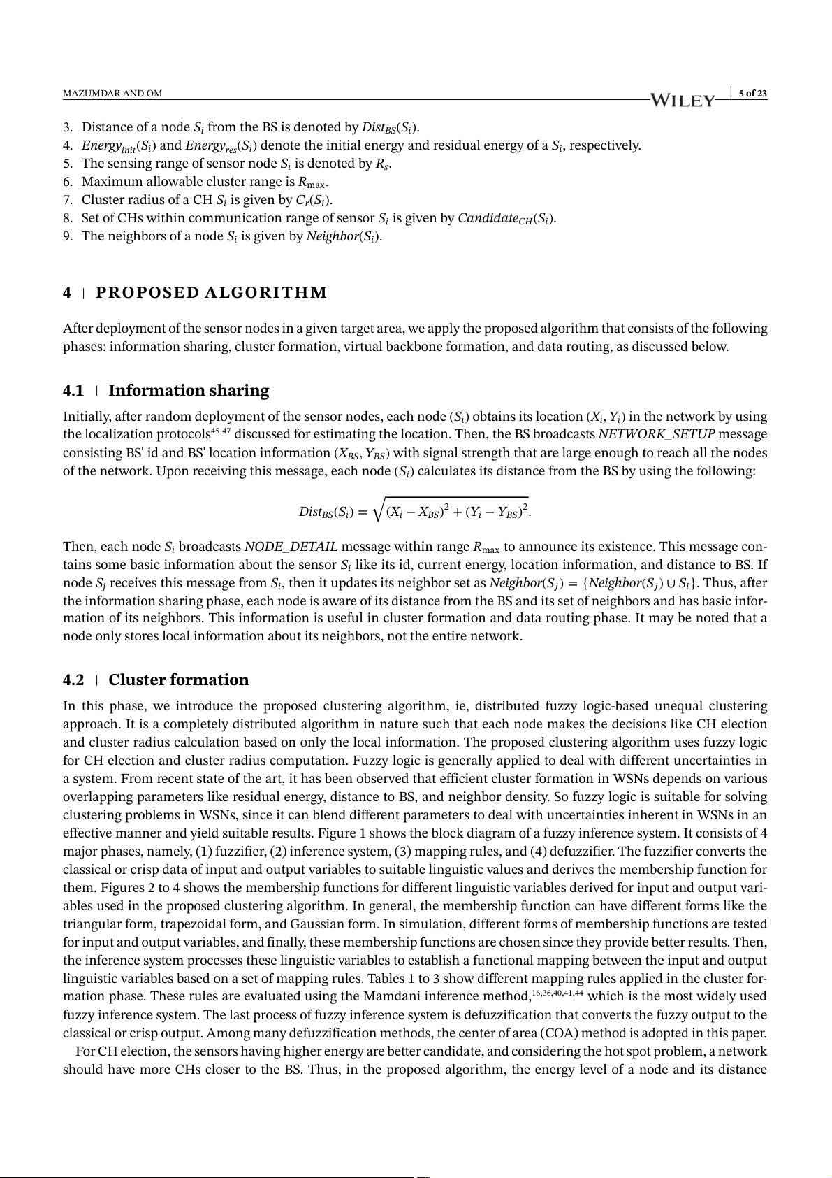
effective manner and yield suitable results. Figure 1 shows the block diagram of a fuzzy inference system. It consists of 4
major phases, namely, (1) fuzzifier, (2) inference system, (3) mapping rules, and (4) defuzzifier. The fuzzifier converts the
classical or crisp data of input and output variables to suitable linguistic values and derives the membership function for
them. Figures 2 to 4 shows the membership functions for different linguistic variables derived for input and output vari-
ables used in the proposed clustering algorithm. In general, the membership function can have different forms like the
triangular form, trapezoidal form, and Gaussian form. In simulation, different forms of membership functions are tested
for input and output variables, and finally, these membership functions are chosen since they provide better results. Then,
the inference system processes these linguistic variables to establish a functional mapping between the input and output
linguistic variables based on a set of mapping rules. Tables 1 to 3 show different mapping rules applied in the cluster for-
mation phase. These rules are evaluated using the Mamdani inference method,16,36,40,41,44 which is the most widely used
fuzzy inference system. The last process of fuzzy inference system is defuzzification that converts the fuzzy output to the
classical or crisp output. Among many defuzzification methods, the center of area (COA) method is adopted in this paper.
For CH election, the sensors having higher energy are better candidate, and considering the hot spot problem, a network
should have more CHs closer to the BS. Thus, in the proposed algorithm, the energy level of a node and its distance 6 of 23 MAZUMDAR AND OM
FIGURE 1 Block diagram of a fuzzy interface system (A) (B) (C)
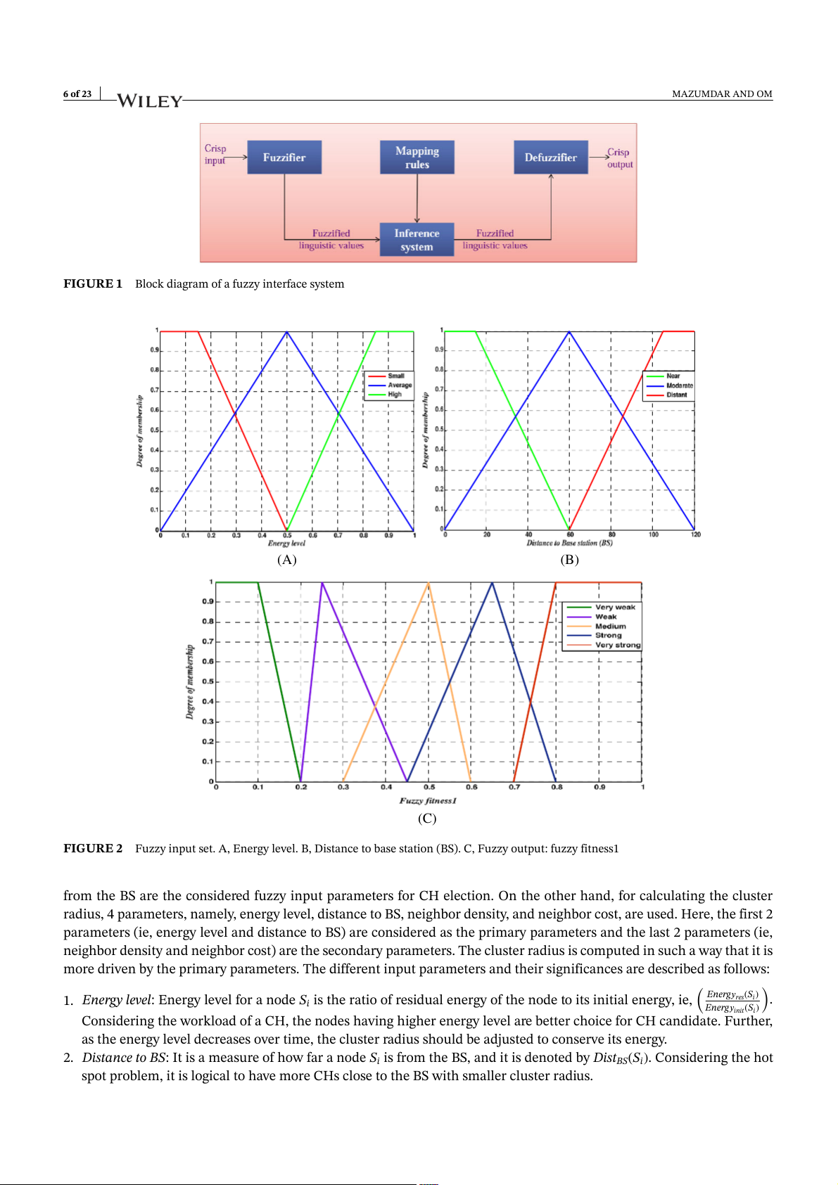
FIGURE 2 Fuzzy input set. A, Energy level. B, Distance to base station (BS). C, Fuzzy output: fuzzy fitness1
from the BS are the considered fuzzy input parameters for CH election. On the other hand, for calculating the cluster
radius, 4 parameters, namely, energy level, distance to BS, neighbor density, and neighbor cost, are used. Here, the first 2
parameters (ie, energy level and distance to BS) are considered as the primary parameters and the last 2 parameters (ie,
neighbor density and neighbor cost) are the secondary parameters. The cluster radius is computed in such a way that it is
more driven by the primary parameters. The different input parameters and their significances are described as follows: ( )
1. Energy level: Energy level for a node S Energ𝑦 S res( i)
i is the ratio of residual energy of the node to its initial energy, ie, .
Energ𝑦init(Si)
Considering the workload of a CH, the nodes having higher energy level are better choice for CH candidate. Further,
as the energy level decreases over time, the cluster radius should be adjusted to conserve its energy.
2. Distance to BS: It is a measure of how far a node Si is from the BS, and it is denoted by DistBS(Si). Considering the hot
spot problem, it is logical to have more CHs close to the BS with smaller cluster radius. MAZUMDAR AND OM 7 of 23 (A) (B) (C)
FIGURE 3 Fuzzy input set. A, Neighbor density. B, Neighbor cost. C, Fuzzy output: fuzzy fitness2
FIGURE 4 Fuzzy set for output variable cluster radius
3. Neighbor density: For a node Si, it is the ratio of the number of neighbors of Si to the total number of nodes (N) in the ( ) network, ie, Neigh
|Neighbor(S )i| Densit
. Considering the unpredictability of random deployment of sensor nodes, 𝑦(Si) = N
it is possible that in spite of smaller cluster radius of a CH closer to the BS, it might have more CMs than the CHs farther
from the BS that have larger cluster radii. Such facts might significantly degrade the advantages the unequal clustering
can offer. So the parameter like node degree is a better choice to be considered in cluster radius computation.
4. Neighbor cost: As the cluster radius increases, the intracluster communication cost increases. So while calculating the
cluster radius for a CH, the neighbors communication cost should also be considered. Since the energy dissipated 8 of 23 MAZUMDAR AND OM
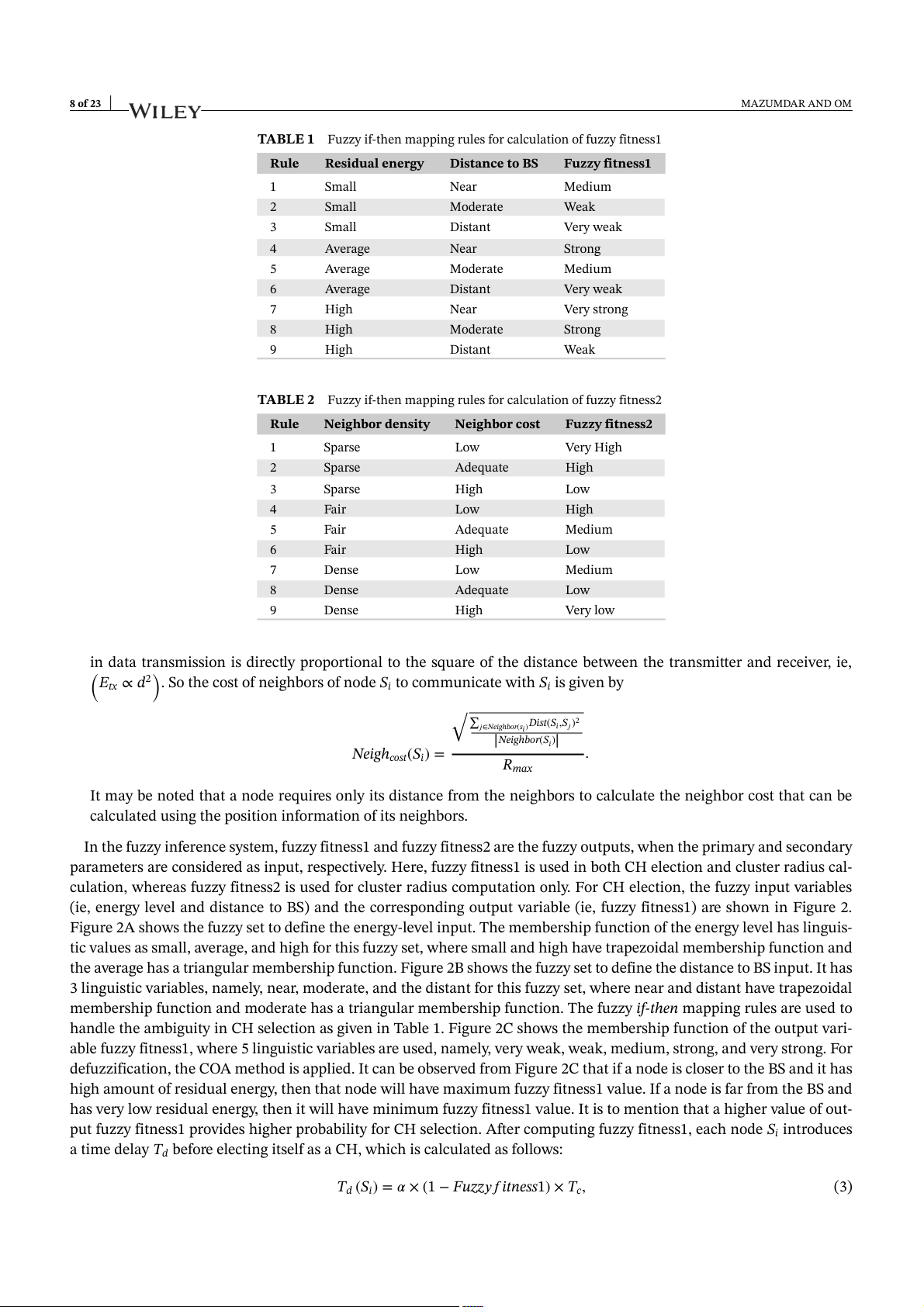
TABLE 1 Fuzzy if-then mapping rules for calculation of fuzzy fitness1 Rule Residual energy Distance to BS Fuzzy fitness1 1 Small Near Medium 2 Small Moderate Weak 3 Small Distant Very weak 4 Average Near Strong 5 Average Moderate Medium 6 Average Distant Very weak 7 High Near Very strong 8 High Moderate Strong 9 High Distant Weak
TABLE 2 Fuzzy if-then mapping rules for calculation of fuzzy fitness2 Rule Neighbor density Neighbor cost Fuzzy fitness2 1 Sparse Low Very High 2 Sparse Adequate High 3 Sparse High Low 4 Fair Low High 5 Fair Adequate Medium 6 Fair High Low 7 Dense Low Medium 8 Dense Adequate Low 9 Dense High Very low
in data transmission is directly proportional to the square of the distance between the transmitter and receiver, ie, ( )
Etx ∝ d2 . So the cost of neighbors of node Si to communicate with Si is given by √∑ Dist(S )2
𝑗∈Neighbor(si) i,S𝑗 |Neighbor(Si)| Neighcost(Si) = . Rmax
It may be noted that a node requires only its distance from the neighbors to calculate the neighbor cost that can be
calculated using the position information of its neighbors.
In the fuzzy inference system, fuzzy fitness1 and fuzzy fitness2 are the fuzzy outputs, when the primary and secondary
parameters are considered as input, respectively. Here, fuzzy fitness1 is used in both CH election and cluster radius cal-
culation, whereas fuzzy fitness2 is used for cluster radius computation only. For CH election, the fuzzy input variables
(ie, energy level and distance to BS) and the corresponding output variable (ie, fuzzy fitness1) are shown in Figure 2.
Figure 2A shows the fuzzy set to define the energy-level input. The membership function of the energy level has linguis-
tic values as small, average, and high for this fuzzy set, where small and high have trapezoidal membership function and
the average has a triangular membership function. Figure 2B shows the fuzzy set to define the distance to BS input. It has
3 linguistic variables, namely, near, moderate, and the distant for this fuzzy set, where near and distant have trapezoidal
membership function and moderate has a triangular membership function. The fuzzy if-then mapping rules are used to
handle the ambiguity in CH selection as given in Table 1. Figure 2C shows the membership function of the output vari-
able fuzzy fitness1, where 5 linguistic variables are used, namely, very weak, weak, medium, strong, and very strong. For
defuzzification, the COA method is applied. It can be observed from Figure 2C that if a node is closer to the BS and it has
high amount of residual energy, then that node will have maximum fuzzy fitness1 value. If a node is far from the BS and
has very low residual energy, then it will have minimum fuzzy fitness1 value. It is to mention that a higher value of out-
put fuzzy fitness1 provides higher probability for CH selection. After computing fuzzy fitness1, each node Si introduces
a time delay Td before electing itself as a CH, which is calculated as follows:
Td (Si) = 𝛼 × (1 − Fuzz𝑦𝑓 itness1) × Tc, (3) MAZUMDAR AND OM 9 of 23
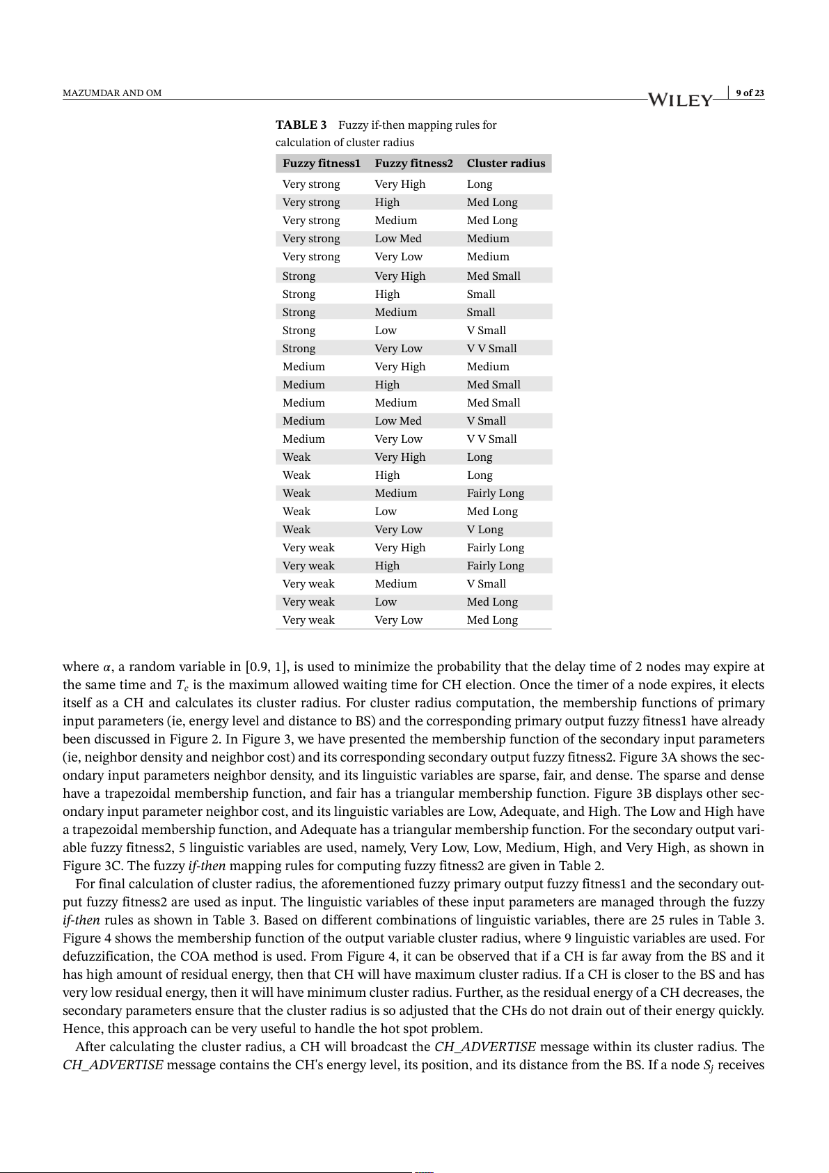
TABLE 3 Fuzzy if-then mapping rules for calculation of cluster radius Fuzzy fitness1 Fuzzy fitness2 Cluster radius Very strong Very High Long Very strong High Med Long Very strong Medium Med Long Very strong Low Med Medium Very strong Very Low Medium Strong Very High Med Small Strong High Small Strong Medium Small Strong Low V Small Strong Very Low V V Small Medium Very High Medium Medium High Med Small Medium Medium Med Small Medium Low Med V Small Medium Very Low V V Small Weak Very High Long Weak High Long Weak Medium Fairly Long Weak Low Med Long Weak Very Low V Long Very weak Very High Fairly Long Very weak High Fairly Long Very weak Medium V Small Very weak Low Med Long Very weak Very Low Med Long
where 𝛼, a random variable in [0.9, 1], is used to minimize the probability that the delay time of 2 nodes may expire at
the same time and Tc is the maximum allowed waiting time for CH election. Once the timer of a node expires, it elects
itself as a CH and calculates its cluster radius. For cluster radius computation, the membership functions of primary
input parameters (ie, energy level and distance to BS) and the corresponding primary output fuzzy fitness1 have already
been discussed in Figure 2. In Figure 3, we have presented the membership function of the secondary input parameters
(ie, neighbor density and neighbor cost) and its corresponding secondary output fuzzy fitness2. Figure 3A shows the sec-
ondary input parameters neighbor density, and its linguistic variables are sparse, fair, and dense. The sparse and dense
have a trapezoidal membership function, and fair has a triangular membership function. Figure 3B displays other sec-
ondary input parameter neighbor cost, and its linguistic variables are Low, Adequate, and High. The Low and High have
a trapezoidal membership function, and Adequate has a triangular membership function. For the secondary output vari-
able fuzzy fitness2, 5 linguistic variables are used, namely, Very Low, Low, Medium, High, and Very High, as shown in
Figure 3C. The fuzzy if-then mapping rules for computing fuzzy fitness2 are given in Table 2.
For final calculation of cluster radius, the aforementioned fuzzy primary output fuzzy fitness1 and the secondary out-
put fuzzy fitness2 are used as input. The linguistic variables of these input parameters are managed through the fuzzy
if-then rules as shown in Table 3. Based on different combinations of linguistic variables, there are 25 rules in Table 3.
Figure 4 shows the membership function of the output variable cluster radius, where 9 linguistic variables are used. For
defuzzification, the COA method is used. From Figure 4, it can be observed that if a CH is far away from the BS and it
has high amount of residual energy, then that CH will have maximum cluster radius. If a CH is closer to the BS and has
very low residual energy, then it will have minimum cluster radius. Further, as the residual energy of a CH decreases, the
secondary parameters ensure that the cluster radius is so adjusted that the CHs do not drain out of their energy quickly.
Hence, this approach can be very useful to handle the hot spot problem.
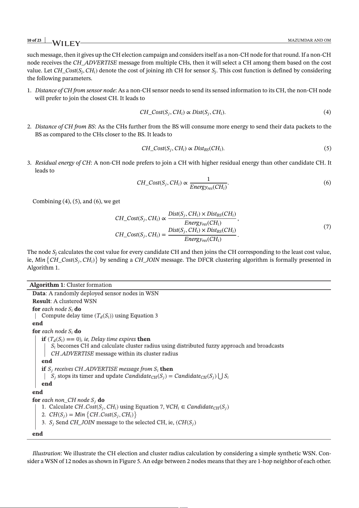
After calculating the cluster radius, a CH will broadcast the CH_ADVERTISE message within its cluster radius. The
CH_ADVERTISE message contains the CH's energy level, its position, and its distance from the BS. If a node Sj receives 10 of 23 MAZUMDAR AND OM
such message, then it gives up the CH election campaign and considers itself as a non-CH node for that round. If a non-CH
node receives the CH_ADVERTISE message from multiple CHs, then it will select a CH among them based on the cost
value. Let CH_Cost(Sj, CHi) denote the cost of joining ith CH for sensor Sj. This cost function is defined by considering the following parameters.
1. Distance of CH from sensor node: As a non-CH sensor needs to send its sensed information to its CH, the non-CH node
will prefer to join the closest CH. It leads to
CH_Cost(S𝑗, CHi) ∝ Dist(S𝑗, CHi). (4)
2. Distance of CH from BS: As the CHs further from the BS will consume more energy to send their data packets to the
BS as compared to the CHs closer to the BS. It leads to
CH_Cost(S𝑗, CHi) ∝ DistBS(CHi). (5)
3. Residual energy of CH: A non-CH node prefers to join a CH with higher residual energy than other candidate CH. It leads to 1
CH_Cost(S𝑗, CHi) ∝ . (6)
Energ𝑦res(CHi)
Combining (4), (5), and (6), we get Dist(S i) × BS( i) CH_Cost 𝑗 , CH Dist CH (S𝑗, CHi) ∝ ,
Energ𝑦res(CHi) (7) Dist(S i) × BS( i) CH_Cost 𝑗 , CH Dist CH (S𝑗, CHi) = .
Energ𝑦res(CHi)
The node Sj calculates the cost value for every candidate CH and then joins the CH corresponding to the least cost value, { }
ie, Min CH_Cost(S𝑗, CHi) by sending a CH_JOIN message. The DFCR clustering algorithm is formally presented in Algorithm 1.
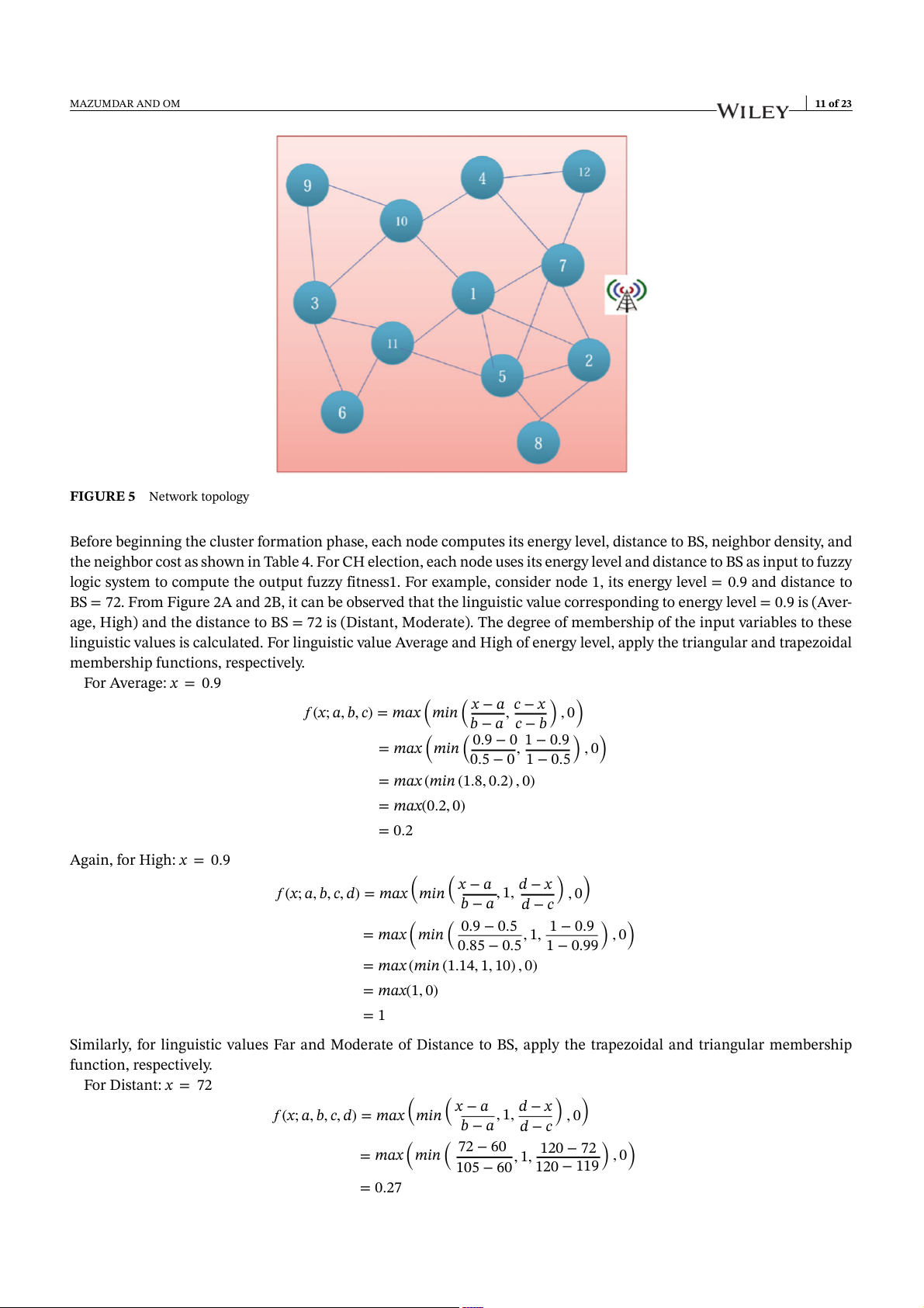
Illustration: We illustrate the CH election and cluster radius calculation by considering a simple synthetic WSN. Con-
sider a WSN of 12 nodes as shown in Figure 5. An edge between 2 nodes means that they are 1-hop neighbor of each other. MAZUMDAR AND OM 11 of 23
FIGURE 5 Network topology
Before beginning the cluster formation phase, each node computes its energy level, distance to BS, neighbor density, and
the neighbor cost as shown in Table 4. For CH election, each node uses its energy level and distance to BS as input to fuzzy
logic system to compute the output fuzzy fitness1. For example, consider node 1, its energy level = 0.9 and distance to
BS = 72. From Figure 2A and 2B, it can be observed that the linguistic value corresponding to energy level = 0.9 is (Aver-
age, High) and the distance to BS = 72 is (Distant, Moderate). The degree of membership of the input variables to these
linguistic values is calculated. For linguistic value Average and High of energy level, apply the triangular and trapezoidal
membership functions, respectively.
For Average: x = 0.9 ( ( ) )
x − a c − x
𝑓 (x; a, b, c) = max min , , 0
b − a c − b ( ( ) )
0.9 − 0 1 − 0.9 = max min , , 0
0.5 − 0 1 − 0.5
= max (min (1.8, 0.2) , 0)
= max(0.2, 0) = 0.2
Again, for High: x = 0.9 ( ( ) ) x − a d − x
𝑓 (x; a, b, c, d) = max min , 1, , 0 b − a d − c ( ( ) ) 0.9 − 0.5 1 − 0.9 = max min , 1, , 0 0.85 − 0.5 1 − 0.99
= max (min (1.14, 1, 10) , 0) = max(1, 0) = 1
Similarly, for linguistic values Far and Moderate of Distance to BS, apply the trapezoidal and triangular membership function, respectively. For Distant: x = 72 ( ( ) ) x − a d − x
𝑓 (x; a, b, c, d) = max min , 1, , 0 b − a d − c ( ( ) ) 72 − 60 120 − 72 = max min , 1, , 0 105 − 60 120 − 119 = 0.27 12 of 23 MAZUMDAR AND OM s iu d ra r ste lu C - - - - - - 5.6 15.5 - 18 16 - ss2 e fitn zzy u F - - - - - - 0.3 0.67 - 0.58 0.64 - (i) d T 4.9 6.4 12.4 8.4 6.8 11.6 2.7 4.6 11.2 3.7 4.4 3.6 ss1 e fitn zzy u F 0.74 0.68 0.38 0.58 0.66 0.42 0.92 0.73 0.44 0.87 0.77 0.82 st co r o b h ig e N 0.55 0.67 0.51 0.58 0.42 0.63 0.18 0.29 0.48 0.31 0.37 0.46 sity n e d r o b h ig e N 0.42 0.33 0.33 0.25 0.25 0.17 0.42 0.17 0.17 0.33 0.33 0.17 S B to ce n ista D 72 17 108 66 79 115 14 52 112 89 93 38 n l atio e v n. rm le fo y rg statio e es'in n ase d E 0.90 0.85 0.77 0.72 0.84 0.88 0.93 0.91 0.80 0.79 0.87 0.86 o S,b N B (i) 4 n: E id L e B d o reviatio A b b T N 1 2 3 4 5 6 7 8 9 10 11 12 A MAZUMDAR AND OM 13 of 23
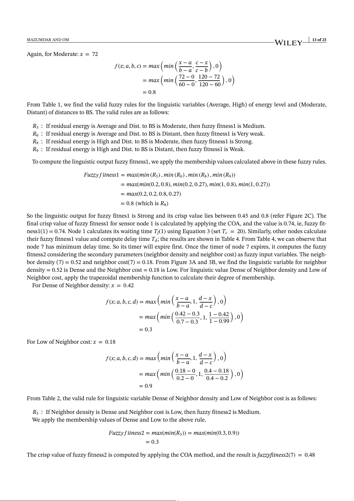
Again, for Moderate: x = 72 ( ( ) )
x − a c − x
𝑓 (x; a, b, c) = max min , , 0
b − a c − b ( ( ) ) 72 − 0 120 − 72 = max min , , 0 60 − 0 120 − 60 = 0.8
From Table 1, we find the valid fuzzy rules for the linguistic variables (Average, High) of energy level and (Moderate,
Distant) of distances to BS. The valid rules are as follows:
R5 ∶ If residual energy is Average and Dist. to BS is Moderate, then fuzzy fitness1 is Medium.
R6 ∶ If residual energy is Average and Dist. to BS is Distant, then fuzzy fitness1 is Very weak.
R8 ∶ If residual energy is High and Dist. to BS is Moderate, then fuzzy fitness1 is Strong.
R9 ∶ If residual energy is High and Dist. to BS is Distant, then fuzzy fitness1 is Weak.
To compute the linguistic output fuzzy fitness1, we apply the membership values calculated above in these fuzzy rules.
Fuzz𝑦𝑓 itness1 = max(min (R5) , min (R6) , min (R8) , min (R9))
= max(min(0.2, 0.8), min(0.2, 0.27), min(1, 0.8), min(1, 0.27))
= max(0.2, 0.2, 0.8, 0.27)
= 0.8 (which is R8)
So the linguistic output for fuzzy fitnes1 is Strong and its crisp value lies between 0.45 and 0.8 (refer Figure 2C). The
final crisp value of fuzzy fitness1 for sensor node 1 is calculated by applying the COA, and the value is 0.74, ie, fuzzy fit-
ness1(1) = 0.74. Node 1 calculates its waiting time Tf(1) using Equation 3 (set Tc = 20). Similarly, other nodes calculate
their fuzzy fitness1 value and compute delay time Td; the results are shown in Table 4. From Table 4, we can observe that
node 7 has minimum delay time. So its timer will expire first. Once the timer of node 7 expires, it computes the fuzzy
fitness2 considering the secondary parameters (neighbor density and neighbor cost) as fuzzy input variables. The neigh-
bor density (7) = 0.52 and neighbor cost(7) = 0.18. From Figure 3A and 3B, we find the linguistic variable for neighbor
density = 0.52 is Dense and the Neighbor cost = 0.18 is Low. For linguistic value Dense of Neighbor density and Low of
Neighbor cost, apply the trapezoidal membership function to calculate their degree of membership.
For Dense of Neighbor density: x = 0.42 ( ( ) ) x − a d − x
𝑓 (x; a, b, c, d) = max min , 1, , 0 b − a d − c ( ( ) ) 0.42 − 0.3 1 − 0.42 = max min , 1, , 0 0.7 − 0.3 1 − 0.99 = 0.3
For Low of Neighbor cost: x = 0.18 ( ( ) ) x − a d − x
𝑓 (x; a, b, c, d) = max min , 1, , 0 b − a d − c ( ( ) ) 0.18 − 0 0.4 − 0.18 = max min , 1, , 0 0.2 − 0 0.4 − 0.2 = 0.9
From Table 2, the valid rule for linguistic variable Dense of Neighbor density and Low of Neighbor cost is as follows:
R5 ∶ If Neighbor density is Dense and Neighbor cost is Low, then fuzzy fitness2 is Medium.
We apply the membership values of Dense and Low to the above rule.
Fuzz𝑦𝑓 itness2 = max(min(R5)) = max(min(0.3, 0.9)) = 0.3
The crisp value of fuzzy fitness2 is computed by applying the COA method, and the result is fuzzyfitness2(7) = 0.48 14 of 23 MAZUMDAR AND OM
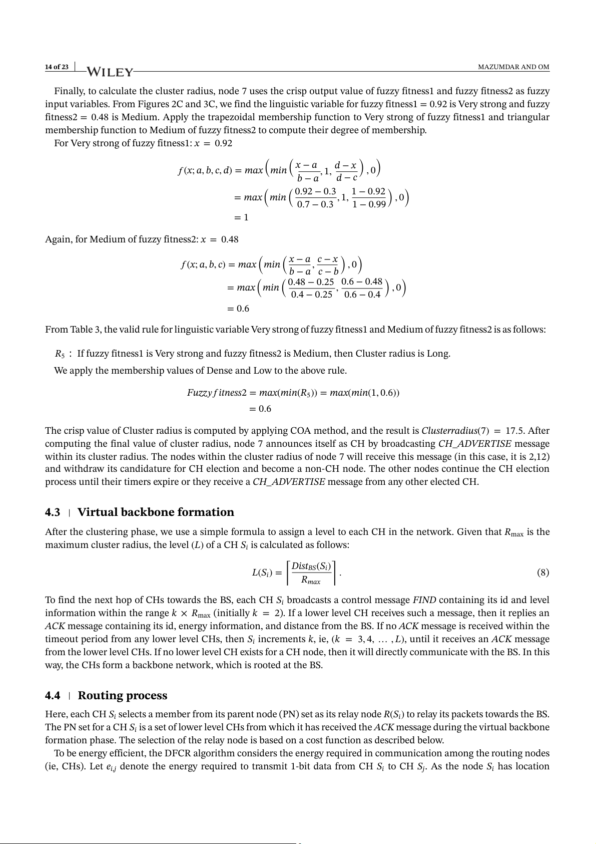
Finally, to calculate the cluster radius, node 7 uses the crisp output value of fuzzy fitness1 and fuzzy fitness2 as fuzzy
input variables. From Figures 2C and 3C, we find the linguistic variable for fuzzy fitness1 = 0.92 is Very strong and fuzzy
fitness2 = 0.48 is Medium. Apply the trapezoidal membership function to Very strong of fuzzy fitness1 and triangular
membership function to Medium of fuzzy fitness2 to compute their degree of membership.
For Very strong of fuzzy fitness1: x = 0.92 ( ( ) ) x − a d − x
𝑓 (x; a, b, c, d) = max min , 1, , 0 b − a d − c ( ( ) ) 0.92 − 0.3 1 − 0.92 = max min , 1, , 0 0.7 − 0.3 1 − 0.99 = 1
Again, for Medium of fuzzy fitness2: x = 0.48 ( ( ) )
x − a c − x
𝑓 (x; a, b, c) = max min , , 0
b − a c − b ( ( ) )
0.48 − 0.25 0.6 − 0.48 = max min , , 0 0.4 − 0.25 0.6 − 0.4 = 0.6
From Table 3, the valid rule for linguistic variable Very strong of fuzzy fitness1 and Medium of fuzzy fitness2 is as follows:
R5 ∶ If fuzzy fitness1 is Very strong and fuzzy fitness2 is Medium, then Cluster radius is Long.
We apply the membership values of Dense and Low to the above rule.
Fuzz𝑦𝑓 itness2 = max(min(R5)) = max(min(1, 0.6)) = 0.6
The crisp value of Cluster radius is computed by applying COA method, and the result is Clusterradius(7) = 17.5. After
computing the final value of cluster radius, node 7 announces itself as CH by broadcasting CH_ADVERTISE message
within its cluster radius. The nodes within the cluster radius of node 7 will receive this message (in this case, it is 2,12)
and withdraw its candidature for CH election and become a non-CH node. The other nodes continue the CH election
process until their timers expire or they receive a CH_ADVERTISE message from any other elected CH. 4.3
Virtual backbone formation
After the clustering phase, we use a simple formula to assign a level to each CH in the network. Given that Rmax is the
maximum cluster radius, the level (L) of a CH Si is calculated as follows: ⌈ ⌉ Dist L BS(Si) (Si) = . (8) Rmax
To find the next hop of CHs towards the BS, each CH Si broadcasts a control message FIND containing its id and level
information within the range k × Rmax (initially k = 2). If a lower level CH receives such a message, then it replies an
ACK message containing its id, energy information, and distance from the BS. If no ACK message is received within the
timeout period from any lower level CHs, then Si increments k, ie, (k = 3, 4, … , L), until it receives an ACK message
from the lower level CHs. If no lower level CH exists for a CH node, then it will directly communicate with the BS. In this
way, the CHs form a backbone network, which is rooted at the BS. 4.4 Routing process
Here, each CH Si selects a member from its parent node (PN) set as its relay node R(Si) to relay its packets towards the BS.
The PN set for a CH Si is a set of lower level CHs from which it has received the ACK message during the virtual backbone
formation phase. The selection of the relay node is based on a cost function as described below.
To be energy efficient, the DFCR algorithm considers the energy required in communication among the routing nodes
(ie, CHs). Let ei,j denote the energy required to transmit 1-bit data from CH Si to CH Sj. As the node Si has location MAZUMDAR AND OM 15 of 23
information of Sj, Si can compute the distance between Si and Sj that is given by Dist(Si, Sj). So ei,j can be calculated using
Equation 1. Let er be the energy required for receiving 1-bit information, and it can be computed from Equation 2. Thus,
the total energy consumed in communication of a data packet of 𝜂 bits is given by ( )
TEi,𝑗 = ei,𝑗 + er × 𝜂. (9)
To be energy balanced, the DFCR algorithm considers the energy of lower level CHs for routing data packets via them.
The cost function should sharply increase the cost of the path if the node's remaining energy is small, thereby forcing to
choose a new path having more remaining energy. Thus, the function in which a small change in input variable causes
a large change in the function output is more favorable in WSNs scenario. In both exponential and sine functions, for a
small change in input value, the function output changes a lot. So we put these 2 functions together to construct the cost function as follows: ( ) 1 Wi,𝑗 = ex𝑝 , (10) Sin(𝜙) ( ( )) Energ𝑦 S )
where 𝜙 = 𝜋 − 𝜋 × res ( 𝑗 . 2 Energ𝑦 S init ( 𝑗 )
It maps 𝜙 to [ 𝜋 , 𝜋]. To be both energy efficient and energy balanced, the DFCR algorithm combines Equations 9 and 10 2
to construct a new cost function that is given by
Cost(Si, S𝑗) = TEi,𝑗 × Wi,𝑗. (11)
Using this cost function, the CH Si selects the best candidate to relay its data packet among multiple candidates as follows: { }
R(Si) = min Cost(Si, S𝑗) , ∀S𝑗 ∈ PN(Si). (12)
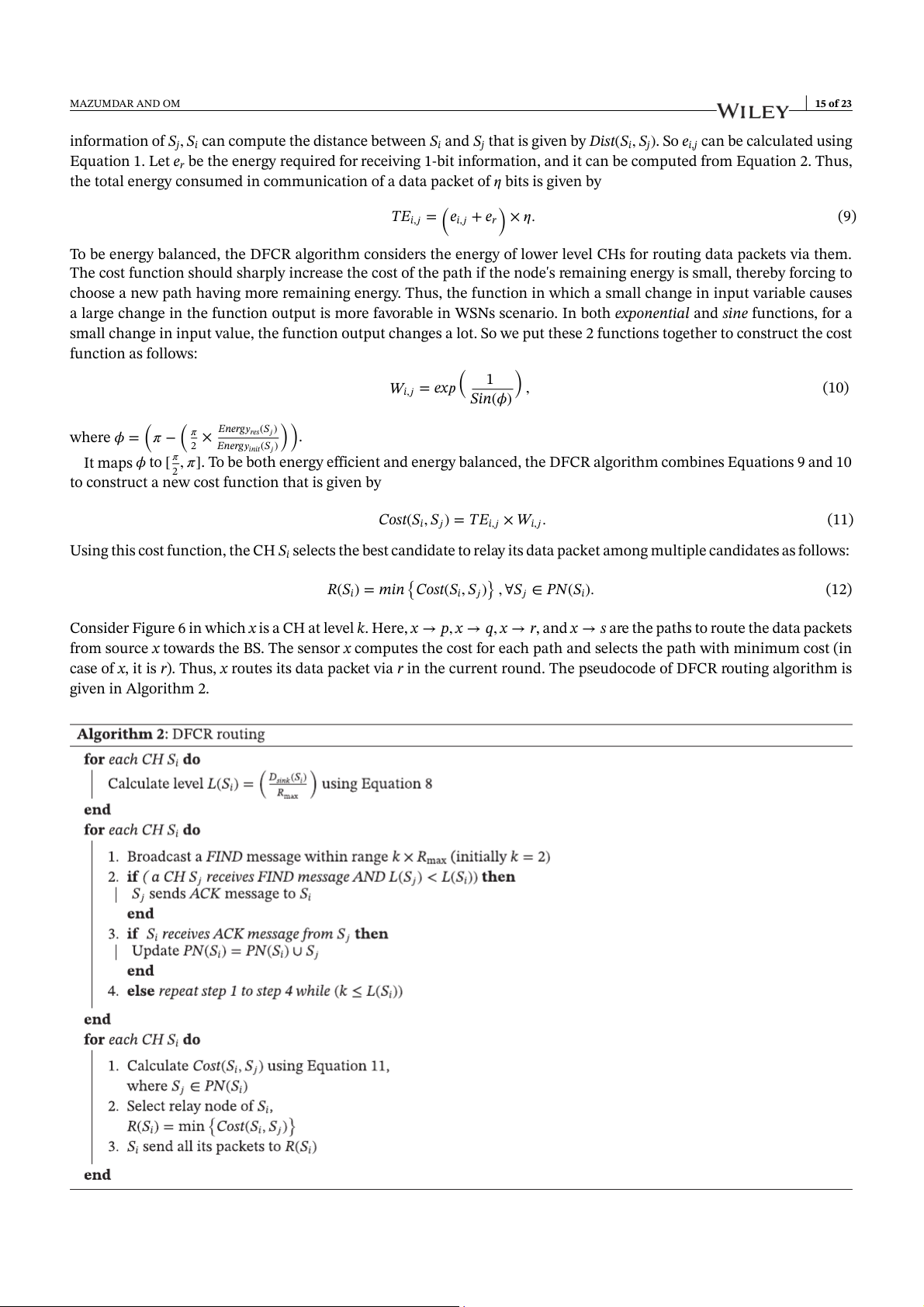
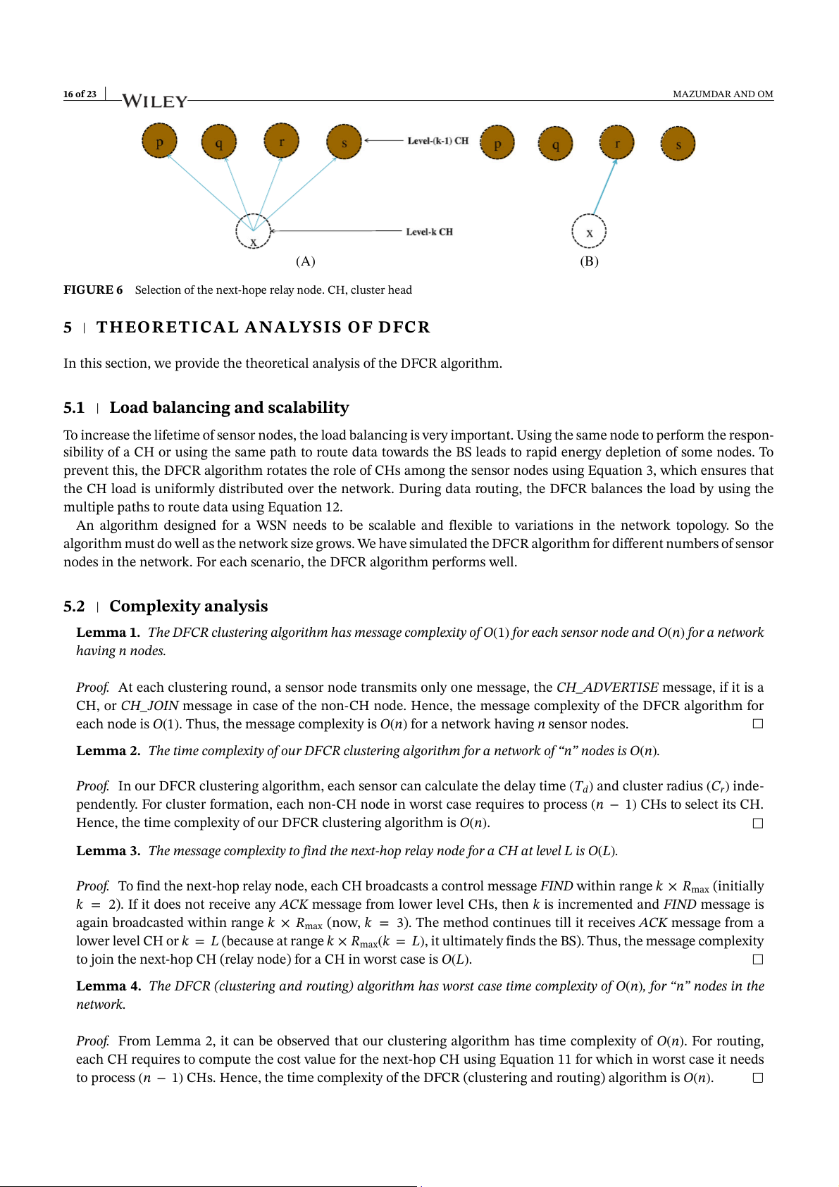
Consider Figure 6 in which x is a CH at level k. Here, x → p, x → q, x → r, and x → s are the paths to route the data packets
from source x towards the BS. The sensor x computes the cost for each path and selects the path with minimum cost (in
case of x, it is r). Thus, x routes its data packet via r in the current round. The pseudocode of DFCR routing algorithm is given in Algorithm 2. 16 of 23 MAZUMDAR AND OM (A) (B)
FIGURE 6 Selection of the next-hope relay node. CH, cluster head 5
THEORETICAL ANALYSIS OF DFCR
In this section, we provide the theoretical analysis of the DFCR algorithm. 5.1
Load balancing and scalability
To increase the lifetime of sensor nodes, the load balancing is very important. Using the same node to perform the respon-
sibility of a CH or using the same path to route data towards the BS leads to rapid energy depletion of some nodes. To
prevent this, the DFCR algorithm rotates the role of CHs among the sensor nodes using Equation 3, which ensures that
the CH load is uniformly distributed over the network. During data routing, the DFCR balances the load by using the
multiple paths to route data using Equation 12.
An algorithm designed for a WSN needs to be scalable and flexible to variations in the network topology. So the
algorithm must do well as the network size grows. We have simulated the DFCR algorithm for different numbers of sensor
nodes in the network. For each scenario, the DFCR algorithm performs well. 5.2 Complexity analysis
Lemma 1. The DFCR clustering algorithm has message complexity of O(1) for each sensor node and O(n) for a network having n nodes.
Proof. At each clustering round, a sensor node transmits only one message, the CH_ADVERTISE message, if it is a
CH, or CH_JOIN message in case of the non-CH node. Hence, the message complexity of the DFCR algorithm for
each node is O(1). Thus, the message complexity is O(n) for a network having n sensor nodes.
Lemma 2. The time complexity of our DFCR clustering algorithm for a network of “n” nodes is O(n).
Proof. In our DFCR clustering algorithm, each sensor can calculate the delay time (Td) and cluster radius (Cr) inde-
pendently. For cluster formation, each non-CH node in worst case requires to process (n − 1) CHs to select its CH.
Hence, the time complexity of our DFCR clustering algorithm is O(n).
Lemma 3. The message complexity to find the next-hop relay node for a CH at level L is O(L).
Proof. To find the next-hop relay node, each CH broadcasts a control message FIND within range k × Rmax (initially
k = 2). If it does not receive any ACK message from lower level CHs, then k is incremented and FIND message is
again broadcasted within range k × Rmax (now, k = 3). The method continues till it receives ACK message from a
lower level CH or k = L (because at range k × Rmax(k = L), it ultimately finds the BS). Thus, the message complexity
to join the next-hop CH (relay node) for a CH in worst case is O(L).
Lemma 4. The DFCR (clustering and routing) algorithm has worst case time complexity of O(n), for “n” nodes in the network.
Proof. From Lemma 2, it can be observed that our clustering algorithm has time complexity of O(n). For routing,
each CH requires to compute the cost value for the next-hop CH using Equation 11 for which in worst case it needs
to process (n − 1) CHs. Hence, the time complexity of the DFCR (clustering and routing) algorithm is O(n). MAZUMDAR AND OM 17 of 23 6 SIMULATION RESULTS
In this section, we perform several experiments to validate the efficiency of the proposed DFCR algorithm. We have
performed experiments using C programming language and MATLAB Fuzzy Toolbox on an Intel i7 processor, 3.40 GHz
CPU, 8 GB RAM running on Windows 7 operating system. The performance of DFCR is evaluated by considering 2
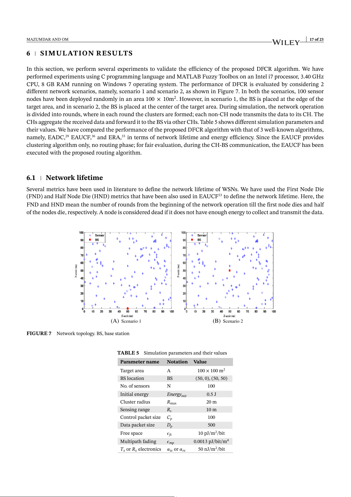
different network scenarios, namely, scenario 1 and scenario 2, as shown in Figure 7. In both the scenarios, 100 sensor
nodes have been deployed randomly in an area 100 × 10m2. However, in scenario 1, the BS is placed at the edge of the
target area, and in scenario 2, the BS is placed at the center of the target area. During simulation, the network operation
is divided into rounds, where in each round the clusters are formed; each non-CH node transmits the data to its CH. The
CHs aggregate the received data and forward it to the BS via other CHs. Table 5 shows different simulation parameters and
their values. We have compared the performance of the proposed DFCR algorithm with that of 3 well-known algorithms,
namely, EADC,29 EAUCF,36 and ERA,33 in terms of network lifetime and energy efficiency. Since the EAUCF provides
clustering algorithm only, no routing phase; for fair evaluation, during the CH-BS communication, the EAUCF has been
executed with the proposed routing algorithm. 6.1 Network lifetime
Several metrics have been used in literature to define the network lifetime of WSNs. We have used the First Node Die
(FND) and Half Node Die (HND) metrics that have been also used in EAUCF33 to define the network lifetime. Here, the
FND and HND mean the number of rounds from the beginning of the network operation till the first node dies and half
of the nodes die, respectively. A node is considered dead if it does not have enough energy to collect and transmit the data. (A) Scenario 1 (B) Scenario 2
FIGURE 7 Network topology. BS, base station
TABLE 5 Simulation parameters and their values Parameter name Notation Value Target area A 100 × 100 m2 BS location BS (50, 0), (50, 50) No. of sensors N 100 Initial energy Energyinit 0.5 J Cluster radius Rmax 20 m Sensing range Rs 10 m Control packet size Cp 100 Data packet size Dp 500 Free space 𝜖fs 10 pJ/m2/bit Multipath fading 𝜖mp 0.0013 pJ/bit/m4
Tx or Rx electronics 𝛼tx or 𝛼rx 50 nJ/m2/bit 18 of 23 MAZUMDAR AND OM 800 1000 DFCR DFCR EAUCF EAUCF 700 900 EADC EADC ERA 800 ERA 600 700 500 600 ds ds n n 400 ou 500 ou R R 400 300 300 200 200 100 100 0 0 Scenario 1 Scenario 2 Scenario 1 Scenario 2
Network scenario
Network scenario (A) FND (B) HND
FIGURE 8 Network lifetime of algorithms. DFCR, distributed fuzzy logic-based unequal clustering approach and routing algorithm;
EADC, energy-aware distributed clustering; EAUCF, energy-aware fuzzy approach to unequal clustering; ERA, energy-aware routing
algorithm; FND, First Node Die; HND, Half Node Die 100 100 DFCR DFCR 90 EAUCF 90 EAUCF EADC EADC 80 ERA 80 ERA ode ode 70 n 70 n sor sor 60 60 50 ive sen 50 ive sen al al 40 40 r of r of be be 30 m 30 m u u N 20 N 20 10 10 0 0 0 100 200 300 400 500 600 700 800 900 0 200 400 600 800 1000 1200 1400 Rounds Rounds (A) Scenario 1 (B) Scenario 2
FIGURE 9 Number of alive nodes per round. DFCR, distributed fuzzy logic-based unequal clustering approach and routing algorithm;
EADC, energy-aware distributed clustering; EAUCF, energy-aware fuzzy approach to unequal clustering; ERA, energy-aware routing algorithm
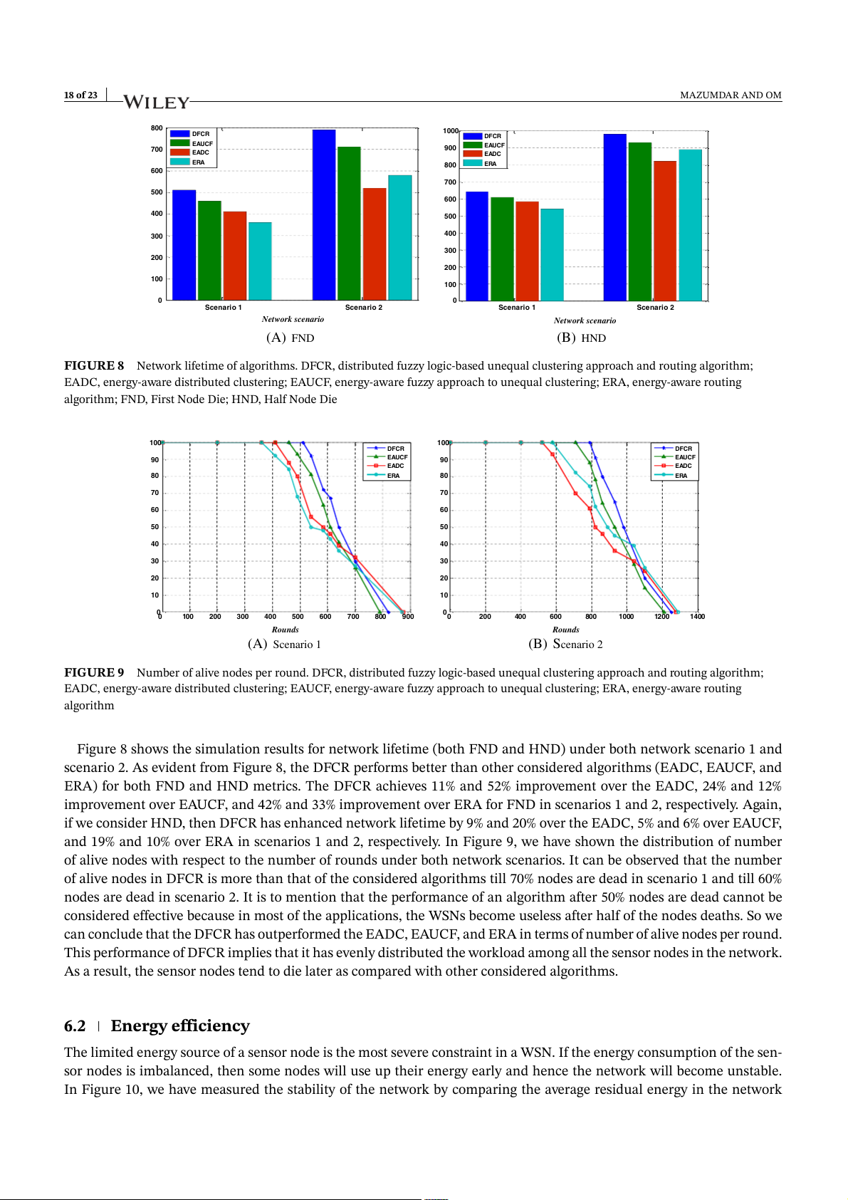
Figure 8 shows the simulation results for network lifetime (both FND and HND) under both network scenario 1 and
scenario 2. As evident from Figure 8, the DFCR performs better than other considered algorithms (EADC, EAUCF, and
ERA) for both FND and HND metrics. The DFCR achieves 11% and 52% improvement over the EADC, 24% and 12%
improvement over EAUCF, and 42% and 33% improvement over ERA for FND in scenarios 1 and 2, respectively. Again,
if we consider HND, then DFCR has enhanced network lifetime by 9% and 20% over the EADC, 5% and 6% over EAUCF,
and 19% and 10% over ERA in scenarios 1 and 2, respectively. In Figure 9, we have shown the distribution of number
of alive nodes with respect to the number of rounds under both network scenarios. It can be observed that the number
of alive nodes in DFCR is more than that of the considered algorithms till 70% nodes are dead in scenario 1 and till 60%
nodes are dead in scenario 2. It is to mention that the performance of an algorithm after 50% nodes are dead cannot be
considered effective because in most of the applications, the WSNs become useless after half of the nodes deaths. So we
can conclude that the DFCR has outperformed the EADC, EAUCF, and ERA in terms of number of alive nodes per round.
This performance of DFCR implies that it has evenly distributed the workload among all the sensor nodes in the network.
As a result, the sensor nodes tend to die later as compared with other considered algorithms. 6.2 Energy efficiency
The limited energy source of a sensor node is the most severe constraint in a WSN. If the energy consumption of the sen-
sor nodes is imbalanced, then some nodes will use up their energy early and hence the network will become unstable.
In Figure 10, we have measured the stability of the network by comparing the average residual energy in the network MAZUMDAR AND OM 19 of 23 0.5 0.5 DFCR DFCR EAUCF EAUCF 0.45 0.45 EADC EADC 0.4 ERA 0.4 ERA y 0.35 y 0.35 erg erg 0.3 0.3 l en l en a a u u 0.25 0.25 0.2 . resid 0.2 . resid vg vg A 0.15 A 0.15 0.1 0.1 0.05 0.05 0 0 0 100 200 300 400 500 600 700 800 900 0 200 400 600 800 1000 1200 1400 Rounds Rounds (A) Scenario 1 (B) Scenario 2
FIGURE 10 Average remaining energy of sensors. DFCR, distributed fuzzy logic-based unequal clustering approach and routing
algorithm; EADC, energy-aware distributed clustering; EAUCF, energy-aware fuzzy approach to unequal clustering; ERA, energy-aware routing algorithm
FIGURE 11 The energy population at 500th round. DFCR, distributed fuzzy logic-based unequal clustering approach and routing
algorithm; EADC, energy-aware distributed clustering; EAUCF, energy-aware fuzzy approach to unequal clustering; ERA, energy-aware routing algorithm
per round. We have performed the experiments for both the scenarios. As it is evident from Figure 10, the DFCR algorithm
consumes less energy as compared with the EADC, EAUCF, and ERA algorithms. Hence, the DFCR has network performance more stable.
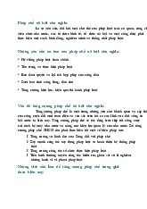
To examine the effect of hot spot problem in DFCR, EADC, EAUCF, and ERA, we have shown in Figure 11 the energy
population of the sensor nodes at round 500 under network scenario 1. As evident from Figure 11, in both EADC and
ERA, most of the nodes closer to the BS have used up their energy due to the hot spot problem. Since none of EADC or
ERA considers any strategy to cope with the hot spot problem, the CHs closer to the BS deplete their energy early due
to heavy data forwarding load towards the BS. On the other hand, both EAUCF and DFCR use unequal cluster strategy
to deal with the hot spot problem. Although the EAUCF forms unequal clusters by considering the residual energy and
distance of a node from the BS, yet it does not consider the intracluster communication cost. Further, in EAUCF, due to
randomized selection of tentative CHs, some low energy nodes may be elected as CHs. The DFCR considers the energy 20 of 23 MAZUMDAR AND OM s,m iu d ra r ste lu .C vg A 12.8 14.4 16.2 17.1 - - s 500 H d C n f u .o o o R N 8 6 5 3 - - s,m iu d ra r ste lu .C g v A 13.7 15.6 17.9 19.2 - - 2 s 100 H rio C a d f n n u .o ce o o S R N 6 5 5 2 - - s,m iu d ra r ste lu .C 500 g d v A 13.2 14.1 14.8 15.9 16.4 17.2 an s 100 H s 500 C d d f n n u u .o ro o o R N 6 5 5 4 3 2 at levels s,m t iu d ra ifferen r d ste at n lu .C atio vg . rm A 14.8 15.3 15.9 16.4 17.3 18.4 ead fo h in 1 s ster 100 H C ster rio a d f ,clu lu n n H C u .o C ce o o N 5 4 4 3 2 2 n: 6 S R E l L e B v e reviatio A L 1 2 3 4 5 6 b b T A
Tài liệu liên quan:
-
Tóm tắt lý thuyết môn IoT và ứng dụng | Học viện Công Nghệ Bưu Chính Viễn Thông
23 12 -
Accelerated Corner-Detector Algorithms: GPU Implementations and Results | Iot và ứng dụng | Học viện Công nghệ Bưu chính Viễn thông
46 23 -
Đề xuất Dự án IoT: Thiết bị phát hiện chạm cho xe máy | Iot và ứng dụng | Học viện Công nghệ Bưu chính Viễn thông
35 18 -
Phân Tích và Giải Pháp FastAPI | Iot và ứng dụng | Học viện Công nghệ Bưu chính Viễn thông
30 15 -
Tăng cường pháp chế xã hội chủ nghĩa trong quản lý nhà nước | Iot và ứng dụng | Học viện Công nghệ Bưu chính Viễn thông
25 13