eleg3124_ch5_laplace_transform

Department of Electrical Engineering University of Arkansas
ELEG 3124 SYSTEMS AND SIGNALS
Ch. 5 Laplace Transform Dr. Jingxian Wu wuj@uark.edu 2 OUTLINE • Introduction • Laplace Transform
• Properties of Laplace Transform
• Inverse Laplace Transform
• Applications of Laplace Transform 3 INTRODUCTION
• Why Laplace transform?
– Frequency domain analysis with Fourier transform is extremely
useful for the studies of signals and LTI system.
• Convolution in time domain ➔ Multiplication in frequency domain.
– Problem: many signals do not have Fourier transform
x(t) = exp(at)u(t), a  0 x(t) = ( tu t)
– Laplace transform can solve this problem
• It exists for most common signals.
• Follow similar property to Fourier transform
• It doesn’t have any physical meaning; just a mathematical tool to facilitate analysis.
– Fourier transform gives us the frequency domain representation of signal. 4 OUTLINE • Introduction • Laplace Transform
• Properties of Laplace Transform
• Inverse Lapalace Transform
• Applications of Fourier Transform 5
LAPLACE TRANSFORM: BILATERAL LAPLACE TRANSFORM
• Bilateral Laplace transform (two-sided Laplace transform) X (s) =
x(t) exp(−st)dt, s =  +  j B +− – s =  +  j is a complex variable
– s is often called the complex frequency – Notations: X (s) = [ L x(t)] B
x(t)  X (s) B
• Time domain v.s. S-domain
– x(t) : a function of time t → x(t) is called the time domain signal
– X (s) : a function of s → X (s) B is called the s-domain signal B
– S-domain is also called as the complex frequency domain 6 LAPLACE TRANSFORM
• Time domain v.s. s-domain
– x(t): a function of time t → x(t) is called the time domain signal
– X (s) : a function of s → X (s) is called the s-domain signal B B
• S-domain is also called the complex frequency domain
– By converting the time domain signal into the s-domain, we can
usually greatly simplify the analysis of the LTI system. – S-domain system analysis:
• 1. Convert the time domain signals to the s-domain with the Laplace transform
• 2. Perform system analysis in the s-domain
• 3. Convert the s-domain results back to the time-domain 7
LAPLACE TRANSFORM: BILATERAL LAPLACE TRANSFORM • Example
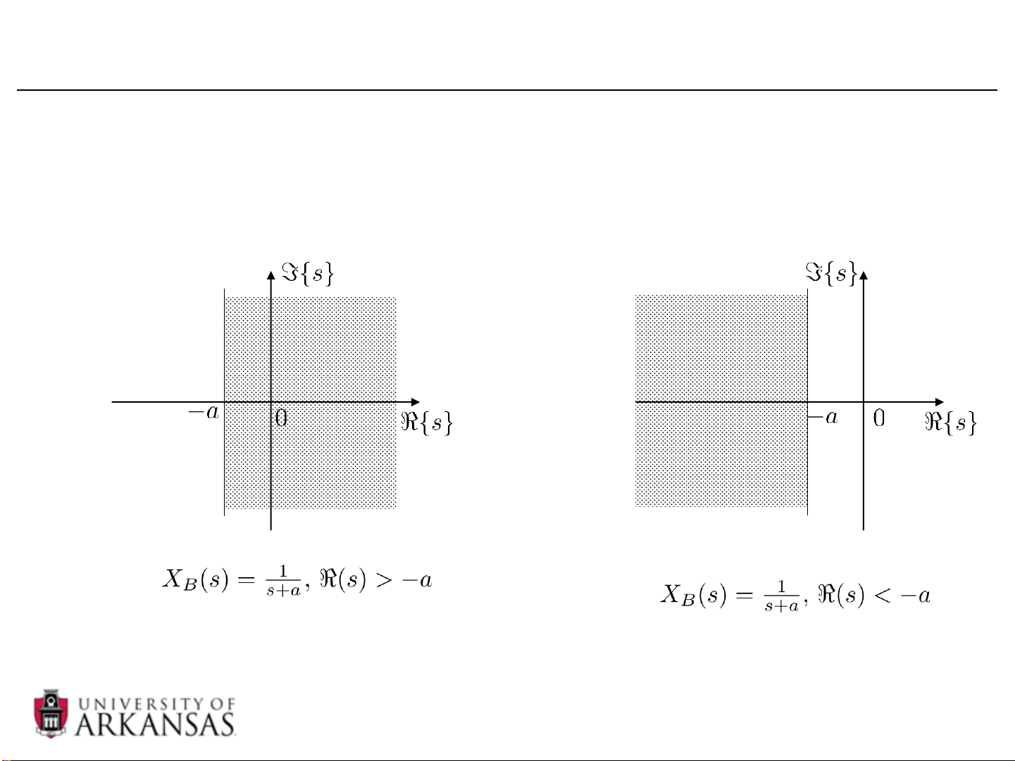
– Find the Bilateral Laplace transform of
x(t) = exp(−at)u(t)
• Region of Convergence (ROC)
– The range of s that the Laplace transform of a signal converges.
– The Laplace transform always contains two components
• The mathematical expression of Laplace transform • ROC. 8
LAPLACE TRANSFORM: BILATERAL LAPLACE TRANSFORM • Example
– Find the Laplace transform of x(t) = −exp(−at)u( t − ) 9
LAPLACE TRANSFORM: BILATERAL LAPLACE TRANSFORM • Example
– Find the Laplace transform of x(t) = 3exp( 2
− t)u(t) + 4exp(t)u( t − ) 10
LAPLACE TRANSFORM: UNILATERAL LAPLACE TRANSFORM
• Unilateral Laplace transform (one-sided Laplace transform)
X (s) = + x(t()ex e p( x −st)dt +−0 – −
0 :The value of x(t) at t = 0 is considered.
– Useful when we dealing with causal signals or causal systems.
• Causal signal: x(t) = 0, t < 0.
• Causal system: h(t) = 0, t < 0.
– We are going to simply call unilateral Laplace transform as Laplace transform. 11
LAPLACE TRANSFORM: UNILATERAL LAPLACE TRANSFORM
• Example: find the unilateral Laplace transform of the following signals. – 1. x t ( ) = A
– 2. x(t) =  (t) 12
LAPLACE TRANSFORM: UNILATERAL LAPLACE TRANSFORM • Example – 3. (
x t) = exp( j2t)
– 4. x(t) = cos(2t) – 5.
x(t) = sin( 2t) 13
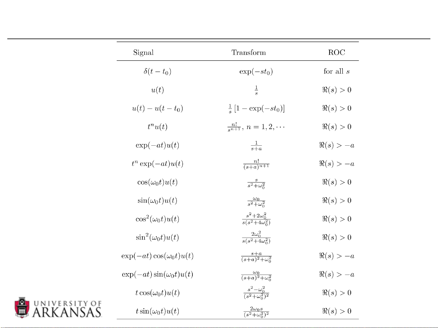
LAPLACE TRANSFORM: UNILATERAL LAPLACE TRANSFORM 14 OUTLINE • Introduction • Laplace Transform
• Properties of Laplace Transform
• Inverse Lapalace Transform
• Applications of Fourier Transform 15 PROPERTIES: LINEARITY • Linearity – 
x (t)  X (s) If x (t) X (s) 1 1 2 2 – Then
ax (t) + bx (t)  aX (s) + bX (s) 1 2 1 2
The ROC is the intersection between the two original signals • Example
– Find the Laplace transfrom of A + B exp( bt − )u(t) 16
PROPERTIES: TIME SHIFTING • Time shifting – If x (t)  X (s and ) t  0 0 – Then (
x t − t )u(t − t )  X (s) exp( st − ) 0 0 0 The ROC remain unchanged 17
PROPERTIES: SHIFTING IN THE s DOMAIN
• Shifting in the s domain Re(s)   –  If x(t) X (s)
– Then y(t) = (
x t) exp(s t)  X (s − s )
Re(s)   + Re(s ) 0 0 0 • Example
– Find the Laplace transform of (
x t) = Aexp( at
− )cos( t)u(t) 0 18
PROPERTIES: TIME SCALING • Time scaling – s   If
x(t)  X (s) Re{ } 1 – Then 1  s  x(at)  X   Re{ } s   a 1 a  a  • Example
– Find the Laplace transform of x(t) = u(at) 19
PROPERTIES: DIFFERENTIATION IN TIME DOMAIN
• Differentiation in time domain – If
g(t)  G(s) – Then
dg(t)  sG(s) g(0− − ) dt 2 d g(t) 2
 s G(s) − sg(0−) − g'(0−) 2 dt n
d g(t)  nsG(s) n 1− − s g(0−) (n−2) −− sg (0− ) (n− ) 1 − g (0− ) n dt • Example – 2 −
Find the Laplace transform of g(t) = sin t  u(t), g(0 ) = 0 20
PROPERTIES: DIFFERENTIATION IN TIME DOMAIN • Example
– Use Laplace transform to solve the differential equation ' −
y''(t) + 3y'(t) + 2y(t) = , 0 0 ( − y ) = 3 y (0 ) = 1