Forecasting with a Bivariate Hysteretic Time Series ModelIncorporating Asymmetric Volatility and Dynamic Correlations
Forecasting with a Bivariate Hysteretic Time Series ModelIncorporating Asymmetric Volatility and Dynamic Correlations. Tài liệu được sưu tầm giúp bạn tham khảo, ôn tập và đạt kết quả cao. Mời bạn đọc đón xem.
Môn: Tài liệu Tổng hợp 3.6 K tài liệu
Trường: Tài liệu khác 3.9 K tài liệu
Tác giả:


Preview text:
Article
Forecasting with a Bivariate Hysteretic Time Series Model
Incorporating Asymmetric Volatility and Dynamic Correlations Hong Thi Than
Faculty of Mathematics and Statistics, Ton Duc Thang University, Ho Chi Minh City 700000, Vietnam; thanthihong@tdtu.edu.vn Abstract
This study explores asymmetric volatility structures within multivariate hysteretic au-
toregressive (MHAR) models that incorporate conditional correlations, aiming to flexibly
capture the dynamic behavior of global financial assets. The proposed framework integrates
regime switching and time-varying delays governed by a hysteresis variable, enabling
the model to account for both asymmetric volatility and evolving correlation patterns
over time. We adopt a fully Bayesian inference approach using adaptive Markov chain
Monte Carlo (MCMC) techniques, allowing for the joint estimation of model parameters,
Value-at-Risk (VaR), and Marginal Expected Shortfall (MES). The accuracy of VaR forecasts
is assessed through two standard backtesting procedures. Our empirical analysis involves
both simulated data and real-world financial datasets to evaluate the model’s effectiveness
in capturing downside risk dynamics. We demonstrate the application of the proposed
method on three pairs of daily log returns involving the S&P500, Bank of America (BAC),
Intercontinental Exchange (ICE), and Goldman Sachs (GS), present the results obtained,
and compare them against the original model framework.
Keywords: bivariate Student’s t-distribution; hysteresis; asymmetry structures in volatility;
Markov chain Monte Carlo; value-at-risk; marginal expected shortfall; out-of-sample forecasting Academic Editor: Boris Ryabko 1. Introduction Received: 26 May 2025
Shocks to a time series can cause persistent effects, whereby the influence of distur- Revised: 16 July 2025
bances spreads and persists over time. This phenomenon, referred to as the hysteresis effect, Accepted: 19 July 2025
reflects a form of path dependence in which system dynamics respond asymmetrically to Published: 21 July 2025
past shocks. To address issues related to excessive or spurious regime shifts, a range of
Citation: Than, H.T. Forecasting with
univariate hysteretic time series models have been developed by the authors of [1–7]. In
a Bivariate Hysteretic Time Series Model Incorporating Asymmetric
financial econometrics, it is well established that asset returns tend to exhibit co-movement.
Volatility and Dynamic Correlations.
Understanding and forecasting the temporal dependence in the second-order moments
Entropy 2025, 27, 771. https://doi.org/
of these returns is a key concern in finance. Multivariate models provide a useful frame- 10.3390/e27070771
work for capturing complex features such as volatility clustering across multiple assets,
Copyright: © 2025 by the authors.
time-varying correlations, and joint downside tail risks across industries. These consid-
Licensee MDPI, Basel, Switzerland.
erations have led researchers to extend univariate volatility models into the multivariate
This article is an open access article
setting. For instance, the authors of [8] introduced the VECH and BEKK models, while
distributed under the terms and
the authors of [9] proposed the Dynamic Conditional Correlation (DCC) model, which
conditions of the Creative Commons
allows for a time-varying conditional correlation matrix. In contrast, the authors of [10] Attribution (CC BY) license (https://creativecommons.org/
developed a model that captures correlation dynamics through a weighted average of past licenses/by/4.0/).
correlation matrices, reflecting the persistence of conditional correlations. The authors Entropy 2025, 27, 771
https://doi.org/10.3390/e27070771 Entropy 2025, 27, 771 2 of 25
of [11] developed an asymmetric Dynamic Conditional Correlation (AG-DCC) model to
examine the presence of asymmetric responses in conditional volatility and correlation
between financial asset returns, particularly allowing for asymmetries in the correlations.
A comprehensive discussion on generalized univariate volatility models can be found
in [12]. The authors of [13] suggested an extension of [10] using a Bayesian Markov chain
Monte Carlo (MCMC) technique to accommodate heavy-tailed distributions. Nonetheless,
these models do not consider regime-switching behavior, which is potentially essential for
modeling structural shifts and regime-dependent dynamics in financial markets.
In the multivariate context, the authors of [14] proposed the Hysteretic Vector Au-
toregressive (HVAR) model, which incorporates delayed regime switching based on a
hysteresis variable. Specifically, transitions between regimes occur only when this variable
exits a predefined hysteresis zone. The authors of [15] introduced a bivariate HAR model
incorporating GARCH errors and time-varying correlations. This model integrates features
of dynamic correlation, asymmetric effects on correlation and volatility, and heavy-tailed
distribution within the multivariate HAR framework previously developed by [14]. How-
ever, the asymmetry in [15] is introduced only through the regime-switching behavior
of a hysteresis variable within the system. This approach overlooks the leverage effects
associated with individual asset returns, which have been emphasized in earlier studies
in [11]. In a univariate framework, the authors of [16,17] examined the intricate dynamics
between financial returns and volatility, emphasizing the asymmetric effects of shocks. The
authors of [16] modified the GARCH model to account for seasonal volatility patterns, dif-
ferential impacts of positive and negative return innovations, and the influence of nominal
interest rates on conditional variance. Similarly, the author of [17] generalized the ARCH
framework by modeling the conditional variance as a quadratic function of past innova-
tions, allowing for a nuanced capture of volatility patterns, including asymmetries and
leverage effects. Both studies underscore the importance of accommodating asymmetries
in volatility modeling to better understand and predict financial market behaviors.
As a result, the volatility specification in [15] leaves room for improvement in modeling
asymmetric effects at the level of individual return series. In this paper, we develop an
extension of the multivariate hysteretic autoregressive (MHAR) model with GARCH errors
and dynamic correlations (see [15]) to accommodate asymmetries in volatility dynamics.
Specifically, we incorporate two well-known asymmetric volatility specifications: the GJR-
GARCH, as defined in [16], and the QGARCH, proposed in [17]. These extensions result in
two model variants, namely, the MHAR–GJR–GARCH and the MHAR–QGARCH models.
To the best of our knowledge, this is the first study to explore asymmetric volatility
structures within the MHAR–GARCH framework. By introducing these asymmetric
components, the proposed models offer greater flexibility in capturing the heterogeneity
and nonlinear behavior commonly observed in financial asset returns. Such flexibility is
particularly important in modeling risk dynamics, especially during periods of market
turbulence where asymmetries in volatility play a crucial role. Based on the proposed
models, we employ an adaptive multivariate t-distribution to account for heavy-tailed
errors, and utilize the SMN representation (see [18]) to flexibly model marginal error
distributions with varying degrees of freedom, improving the model’s fit to the target time series.
In finance, systemic risk refers to the possibility that problems in one financial insti-
tution or a group of them could spread throughout the financial system due to the strong
connections between institutions. Such a chain reaction can lead to serious disruptions or
even cause the entire market to collapse. Following [19], the Marginal Expected Shortfall
(MES) is employed to empirically evaluate the extent to which this risk measure addresses
practical concerns related to systemic risk, using a large sample of major U.S. banks. In this Entropy 2025, 27, 771 3 of 25
study, we consider two widely used risk measures: Value at Risk (VaR) and MES, in which
MES plays a more prominent role in capturing tail risk and systemic vulnerability. Addi-
tionally, we implement two backtesting procedures to assess the accuracy of out-of-sample VaR forecasts.
A major limitation of the proposed models lies in their increasing complexity, partic-
ularly due to the large number of parameters that must be estimated and the challenges
involved in modeling nonlinear multivariate structures. As the nonlinearity and asym-
metric structures of the proposed models increase, traditional estimation methods become
inefficient or impractical. To overcome these difficulties, we adopt a Bayesian framework
using Markov chain Monte Carlo (MCMC) techniques, which allows for simultaneous
inference of all unknown parameters.
The remainder of this paper is divided into the following sections: The multivariate
hysteretic autoregressive model with time-varying correlations and asymmetry structures
in volatility is presented in Section 2. Bayesian inference for the model parameters is
presented in Section 3. Forecasting VaR and the marginal expected shortfall (MES) are
considered in Section 4. Section 5 examines simulation. The empirical study is described in
Section 6 and marks are covered in Section 7.
2. Multivariate Hysteretic Autoregressive Model with Asymmetry
Structures in Volatility and Time-Varying Correlation
We consider the MHAR–GARCH model, a multivariate hysteretic autoregressive model with GARCH type errors: c
yt = Φ(Jt) + ∑ Φ(Jt)y 0 l t−l + at, (1) l=1 q q at = diag h1,t, . . . , hk,t ϵt
where ϵt ∼ D(0, Σt), pi qi ( ( ( h Jt) Jt) Jt) i,t = ω + ∑ a2 + ∑ h i0 αil i,t−l βil i,t−l , i = 1, . . . , k, l=1 l=1 Σ (J t ) (Jt) (Jt) (Jt) t = 1 − θ − Σ(Jt) + Σ Ψ 1 θ2 θ1 t−1 + θ2 t−1, 1 if z t ≤ rL Jt = 2 if zt > rU Jt−1 otherwise, rL < rU,
and the (u, v)th element of Ψt−1 is formulated as: S
∑ ϵu,t−sϵv,t−s s=1 ψuv,t−1 = , 1 ≤ u < v ≤ S⋆ ≤ S. (2) s S S ∑ 2 2 ϵu,t−s ∑ ϵv,t−s s=1 s=1 ′
where yt = (y1,t, . . . , yk,t) is a vector of k assets at time t, Jt is a regime indicator, Φ(Jt) 0
is a k-dimensional vector, Φ(Jt) is a k × k matrix, Σ(Jt) is a k × k positive-definite matrix l (J (J (J
with diagonal elements, scalar parameters are satisfied t ) t ) t ) θ , > 0 and 0 < + 1 θ2 θ1 (Jt) θ < 1, and Ψ 2
t−1 is a k × k sample correlation matrix of shocks from t − S, . . . , t − 1 for
a pre-specified S. Moreover, zt is a hysteresis variable. In this study, we investigate two
distinct forms of asymmetric volatility within the framework of a multivariate hysteretic
autoregressive (MHAR) model. The first approach incorporates the asymmetric volatility
structure proposed by [16] into the MHAR–GARCH framework, resulting in the MHAR– Entropy 2025, 27, 771 4 of 25
GJR–GARCH model. The second approach introduces the quadratic GARCH specification,
as developed by the authors of [17], leading to the formulation of the MHAR–QGARCH
model. We also derive the volatility dynamics of the MHAR–GJR–GARCH model: pi qi ri ( ( ( ( h Jt) Jt) Jt) Jt) i,t = ω + ∑ a2 + ∑ h ∑ I i0 αil i,t−l βil i,t−l + δil
i,t−l {ϵt−l < 0}a2i,t−l, i = 1, ˙ ..., k, l=1 l=1 l=1
where Ii(.) is a k × 1 indicator function that returns a value of 1 when the argument is true
or 0 otherwise. The volatility of the MHAR - QGARCH model is as follows: pi qi ri ( ( ( ( h Jt) Jt) Jt) Jt) i,t = ω + ∑ a2 + ∑ h ∑ a i0 αil i,t−l βil i,t−l + δil i,t−l , i = 1, ˙ ..., k, l=1 l=1 l=1
We now consider the basic cases of two models: the bivariate HAR(1)–GJR–GARCH(1,1)
model and the bivariate HAR(1)–QGARCH(1,1) model. We assume that innovations in
Equation (1) follow the modified bivariate Student’s-t distribution (see [15]). In this case,
we apply the scale SMN representation (see [18]) to the adapted bivariate Student’s-t distribution, T ∗( 2
0, Σt, ν), and we choose zt = y1,t−d. Then, the bivariate HAR(1)–GJR–
GARCH(1,1) model is described as follows:
yt = Φ(Jt) + Φ(Jt)y 0 1 t−1 + at, (3) q q at = diag( h1,t, h2,t)ϵt, ϵt|Λt ∼ N2(0, Λ−1/2Σ ) t tΛ−1/2 t , q Λ1/2 ν ν = i i t diag( λ1,t, pλ2,t), λi,t ∼ Ga , , i = 1, 2, 2 2 Σ (J t ) (Jt) (Jt) (Jt) t = 1 − θ − Σ(Jt) + Σ Ψ 1 θ2 θ1 t−1 + θ2 t−1, 1 if y 1,t−d ≤ rL, Jt = 2 if y1,t−d > rU, Jt−1 otherwise,
where the (u, v)th element of Ψt−1 is described in (2) and the conditional volitilities as follows: ( ( ( ( h Jt) Jt) Jt) Jt) i,t = ω + a2 + h I i0 αi1 i,t−1 βi1 i,t−1 + δi1
i,t−1{ϵt−1 < 0}a2i,t−1, i = 1, 2,
where Ii(.) is a 2 × 1 indicator function that returns a value of 1 when the argument is true
or 0 otherwise. The positivity and stationarity conditions for volatility are given as follows: (Jt) (Jt) (Jt) (Jt) (Jt) (Jt) (Jt) ω > 0, ≥ 0, ≥ 0, ≥ 0 and + + ≤ 1. (4) i0 αi1 βi1 δi1 αi1 βi1 δi1
The bivariate HAR(1)–QGARCH(1,1) model modifies the conditional volatilities as follows: ( ( ( ( h Jt) Jt) Jt) Jt) i,t = ω + a2 + h a i0 αi1 i,t−1 βi1 i,t−1 + δi1 i,t−1, i = 1, 2,
where the positivity and stationarity conditions for volatility are given as follows: (Jt) (Jt) (Jt) (Jt) (Jt) (Jt) (Jt) ω > 0, ≥ 0, ≥ 0, ≥ 0, ( )2 ≤ 4(1 − − ), i0 αi1 βi1 δi1 δi1 αi1 βi1 (J (J and t ) t ) α + ≤ 1, (5) i1 βi1 Entropy 2025, 27, 771 5 of 25
and we specify the unconditional correlation matrix Σ(Jt): " (J # t ) Σ(J 1 ρ t ) = . (J ρ t) 1 3. Bayesian Inference
To estimate the unknown parameters of the proposed models in a Bayesian (J
framework, for example, we create groups of the unknown parameters: (i) t ) ϕ = i ( ( ( ′ ′ ′ ′ ( Jt) Jt) Jt) (1) (2) ϕ , , ) , i, J ; (iii) ; (iv) , ) ; i0 ϕi1 ϕi2
t = 1, 2; (ii) r = (rL, rU )
ν = (ν1, ν2) ρ = (ρ ρ (J (J (J (J (J ′ (J (J ′ (v) t ) t ) t ) t ) t ) (J t ) t ) γ = ( , , , ) , i, J t ) = ( , ) , and (vii) d. We i ωi0 αi1 βi1 δi1
t = 1, 2; (vi) η θ1 θ2
define θ as a vector of all the unknown parameters of the proposed model. Following
that, the bivariate HAR(1)–GJR–GARCH(1,1) and bivariate HAR(1)–QGARCH(1,1) models’
conditional likelihood functions are given by: ( 2 " ! h (Jt)2) ln(L(y| 1,t h2,t (1 − ρ θ)) ∝ ∑ ∑ −0.5 ln (6) t J λ1,tλ2,t t =1 !#) 1 (J p λ λ 2ρ t)a λ − 1t a2 1t + 2ta22t − 1t a2t 1,t λ2,t , p p 2(1 − (J h h h h ρ t)2) 1,t 2,t 1,t 2,t
where at = yt − Φ(Jt) − Φ(Jt)y 0 1 t−1. (J
We set up prior distributions for the unknown parameters. Assume that t ) ϕ ∼ i N3(µ0i, Σ−1), i, J 0i
t = 1, 2; for the threshold parameter rL ∼ Unif(l1, l2), where l1 and l2 are
the pth and (100 − 2p)th percentiles of the observed time series, respectively, for 0 < p < 33.
Furthermore, rU|rL ∼ Unif(u1, u2), where u2 is the (100 − p)th percentile and u1 = rL + c∗
for c∗ is a selected number that ensures rL + c∗ ≤ rU and at least p% of observations are
in the range (rL, rU). For the degrees of freedom, we assume the scale mixture variables (J λ t )
i,t ∼ Ga(νi /2, νi /2) and νi ∼ Unif(2, 60), i = 1, 2, and ρ
∼ Unif(−1, 1). For the lag d,
we choose the discrete uniform prior p(d) = 1/d0 with maximum delay d0. In terms of the (J (J volatility parameters, t ) t ) γ
follows a uniform distribution such that is proportional to i γi
I(S1) or I(S2), where S1 and S2 are the sets that satisfy (4) and (5), respectively.
The conditional posterior distribution for each group is proportional to the conditional
likelihood function multiplied by the prior density for that group, as shown below:
P(θl|y, θ−l) ∝ L(y|θ)P(θl|θ−l),
where θl is each parameter group, P(θl) is its prior density, and θ−l is the vector of all
parameters, except θl. The conditional posterior distribution of the delay lag d follows a
multinomial distribution with a probability:
p(y|d = i, θ Pr(d = i|y, −d)Pr(d = i) θ−d) = , i = 1, . . . , d0. ∑d0 p(y|d = j, j=1 θ−d)Pr(d = j)
In this study, with the exception of the lag parameter d, the conditional posterior
distributions of the remaining parameter groups exhibit non-standard forms. To make a
statistical inference, we employ an adaptive Markov chain Monte Carlo (MCMC) method
for selected parameter groups, complemented by a random walk Metropolis algorithm.
Specifically, we assume that the innovation term in Equation (3) follows a Gaussian distri- (J
bution, which serves as the kernel for sampling t ) (J ϕ . For the parameter groups t ) and i η (Jt) γ , where i, J i
t = 1, 2, an adaptive MCMC approach is utilized to draw samples, whereas
the remaining parameters are updated using the random walk Metropolis algorithm. The Entropy 2025, 27, 771 6 of 25
detailed procedures of the adaptive Metropolis–Hastings MCMC algorithm are thoroughly
presented by the authors of [1,15], where the authors provide a comprehensive framework
for its implementation and application. Following the guidelines of [1], we further adjust
the scale matrix to attain ideal acceptance rates of 20% to 60%.
In a Bayesian framework, we need to set up the initial values for each parameter (J
group. For the autoregressive coefficient parameters, t ) ϕ = (0, 0, 0); for the degrees i (J (J (J (J (J (J of freedom t ) t ) t ) t ) t ) t ) ν = 50; = 0.5; d = = = = 0.1; and i ρi 0 = 3; ωi0 αi1 βi1 δi1 ( ( ( Jt) Jt) θ , ) = (0.05, 0.2) for i, J 1 θ2
t = 1, 2; thresholds rL and rU are established at the 33rd
and 67th percentiles, respectively; and we set p = 20 to make certain of having enough
observations in each regime for a valid inference. For the remainder of the analysis, we specify S = 3.
4. Forecasting the Marginal Expected Shortfall and Value at Risk
The Value-at-Risk (VaR) and Marginal Expected Shortfall (MES) are now considered
systemic risk assessments for financial risk management. The authors of [19] define MES
as a financial firm’s marginal contribution to the financial system’s expected shortfall. The
authors of [20] define MES at the alpha level for a financial institution at time t given Ft−1 as follows:
MESt = E[y2,t | y1,t < VaR1,t(α); Ft−1], (7)
where VaR1,t(α) is the VaR of y1,t at the α-level such that P(y1,t < VaR1,t(α) | Ft−1) = α.
Here, y2,t stands for the stock return of a financial institution, whereas y1,t stands for the market return.
To produce MESt, we estimate one-step-ahead quantiles and volatilities for y1,n+1
from the investigated model described in (3) with forecast origin t = n. We obtain quantiles
from the posterior predictive distribution, which is: Z p(yn+1|Fn) =
p(yn+1|Fn, θ)p(θ|Fn)dθ. (8) θ∈Θ Suppose that { [r] θ
, r = n0 + 1, . . . , N} are the rth MCMC drawn from the posterior [r]
density p(θ|Fn) after the n0 burn-in sample. Thus, we can sample {y , r = n n+1 0 + 1, . . . , N}
from the marginal predictive distribution, p(yn+1|Fn), by sampling the following condi- tional distribution: [ [ y r] |F [r] ∼ T ∗ r] , Σ∗[r] , [r]) n+1 n, θ 2 (µn+1 n+1 ν Z ∞ Z ∞ T ∗ [r] | [r] [r] [r] [r] −1/2 −1/2 Σ∗[r] 2 (y , Σ∗[r] , ) = N y , n+1 µn+1 n+1 ν 2 n+1 µ λ n+1 n+1 n+1λn+1 0 0 2 [r] [r] ! ν ν × ∏ Ga i i λ i,n+1 , dλ 2 2 1,n+1dλ2,n+1, (9) i=1 [r] [r] [r] where µ and Σ∗[r] = diag(h , h
)Σ[r] are a conditional mean and the covariance n+1 n+1 1,n+1 2,n+1 n+1
of p(yn+1|Fn, θ) at the rth iteration. To assess the correctness of a VaR performance, we
calculate the violation rate (VRate). The accuracy of a VaR performance is verified by
recording the failure rate; that is, the violation rate: 1 n+h0 Violation rate = ∑ I(r h t < −VaRt) (10) 0 t=n+1 Entropy 2025, 27, 771 7 of 25
where h0 is the out-of-sample period size and rt is the return at time t. We use two tests to
assess the validity of the VaR forecasts: the conditional coverage (CC) test created by [21]
and the unconditional coverage (UC) test created by [22]. The CC test is conducted to
investigate the null hypothesis that the violations are independently distributed, whereas
the UC test is applied to determine whether the percentage of violations is equivalent to the VaR significance level. 5. Simulation Study
In order to access the effectiveness of the Bayesian approach, we run two simulations
of the suggested models in this section. Model 1 is the bivariate HAR(1)–GJR–GARCH(1,1)
model and Model 2 is the bivariate HAR(1)–QGARCH(1,1) model. Model 1 is given by:
yt = Φ(Jt) + Φ(Jt)y 0 1 t−1 + at, (11) q q at = diag h1,t,
h2,t ϵt, ϵt ∼ T ∗
2 (0, Σt, ν) ϵt|Λt ∼ N2(0, Λ−1/2Σ ) t tΛ−1/2 t , " (1) # " # " # " # − (1) (1) Φ(1) ϕ 0.10 ϕ 0.20 0.25 = 10 = , Φ(1) = 11 ϕ12 = 0 (1) 1 (1) (1) ϕ −0.10 0.25 0.30 20 ϕ21 ϕ22 " (2) # " # " # " # − (2) (2) Φ(2) ϕ 0.08 ϕ 0.30 0.35 = 10 = , Φ(2) = 11 ϕ12 = 0 (2) 1 (2) (2) ϕ −0.15 0.35 0.30 20 ϕ21 ϕ22 ( 0.07 + 0.20a2 + 0.20h if Jt = 1, with h 1,t−1
1,t−1 + 0.40I1,t−1{ϵt−1 < 0}a2 1,t−1 1,t = 0.03 + 0.20a2 + 0.25h if J 1,t−1
1,t−1 + 0.55I1,t−1{ϵt−1 < 0}a2 1,t−1 t = 2, ( 0.04 + 0.25a2 + 0.10h if Jt = 1, h 2,t−1
2,t−1 + 0.40I2,t−1{ϵt−1 < 0}a2 2,t−1 2,t = 0.02 + 0.30a2 + 0.15h if J 2,t−1
2,t−1 + 0.40I2,t−1{ϵt−1 < 0}a2 2,t−1 t = 2, ( Σ
(1 − 0.40 − 0.10)Σ(1) + 0.40Σt−1 + 0.10Ψt−1 if Jt = 1, t =
(1 − 0.50 − 0.20)Σ(2) + 0.50Σt−1 + 0.20Ψt−1 if Jt = 2, 1 if y 1,t−d < −0.5, where Jt = Jt−1 if −0.45 ≤ y1,t−d ≤ 0.1, 2 if y1,t−d > 0.1, " # " # " # " # 1 0.65 1 0.8 ν 8.0 and Σ(1) = , Σ(2) = , 1 ν = = , and d = 1. 0.65 1 0.8 1 ν2 10.0
Model 2 is described as follows:
yt = Φ(Jt) + Φ(Jt)y 0 1 t−1 + at, (12) q q at = diag h1,t,
h2,t ϵt, ϵt ∼ T ∗
2 (0, Σt, ν) " (1) # " # " # " # − (1) (1) Φ(1) ϕ 0.10 ϕ 0.32 0.30 = 10 = , Φ(1) = 11 ϕ12 = 0 (1) 1 (1) (1) ϕ −0.08 0.37 0.35 20 ϕ21 ϕ22 " (2) # " # " # " # − (2) (2) Φ(2) ϕ 0.08 ϕ 0.35 0.30 = 10 = , Φ(2) = 11 ϕ12 = 0 (2) 1 (2) (2) ϕ −0.08 0.33 0.37 20 ϕ21 ϕ22 Entropy 2025, 27, 771 8 of 25 ( 0.07 + 0.20a2 + 0.10h with h 1,t−1 1,t−1 + 0.40a1,t−1 if Jt = 1, 1t = 0.03 + 0.30a2 + 0.10h 1,t−1 1,t−1 + 0.35a1,t−1 if Jt = 2, ( 0.04 + 0.40a2 + 0.05h h 2,t−1 2,t−1 + 0.30a2,t−1 if Jt = 1, 2t = 0.02 + 0.30a2 + 0.10h 2,t−1 2,t−1 + 0.20a2,t−1 if Jt = 2, ( Σ
(1 − 0.40 − 0.35)Σ(1) + 0.40Σt−1 + 0.35Ψt−1 if Jt = 1, t =
(1 − 0.55 − 0.15)Σ(2) + 0.55Σt−1 + 0.15Ψt−1 if Jt = 2, 1 if y 1,t−d < −0.45, where Jt = Jt−1 if −0.45 ≤ y1,t−d ≤ 0.1, 2 if y1,t−d > 0.1, " # " # " # " # 1 0.5 1 0.85 ν 8.0 and Σ(1) = , Σ(2) = , 1 ν = = , and d = 1. 0.5 1 0.85 1 ν2 10.0
Models 1 and 2 are created utilizing the actual values shown in Tables 1 and 2. For each
time series, we set up the sample size n = 2000. We carry out N = 30,000 MCMC iterations
and discard the first M = 10,000 burn-in iterates. For the hyper–parameters, we choose the
initial values for all parameters of the investigated model to be µ = 0i
0, diag(Σ0i) = 0.1,
l1 = ℘20, u2 = ℘80, cL = 2, cU = 60, and d0 = 3.
The results for the parameter estimates of the simulation study are shown in Tables 1 and 2.
The tables present the posterior means, medians, standard deviations, and 95% credible ranges
for Models 1–2 over the 200 replications. We observe that the 95% credible interval contains the
corresponding true value for each parameter. The posterior means and medians in each case are
fairly close to the true parameter values. The posterior modes of lag d are demonstrated, and it
can be explained that the posterior mode of d provides a reliable estimate of the delay parameter
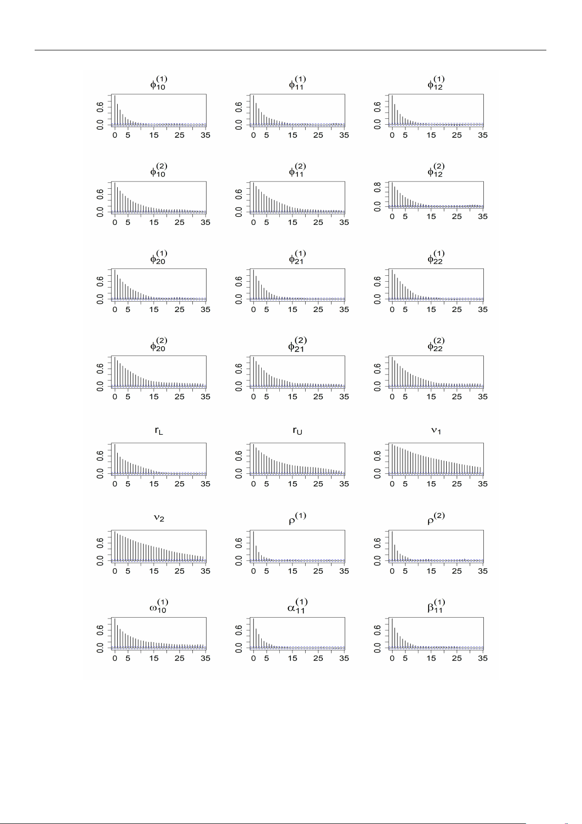
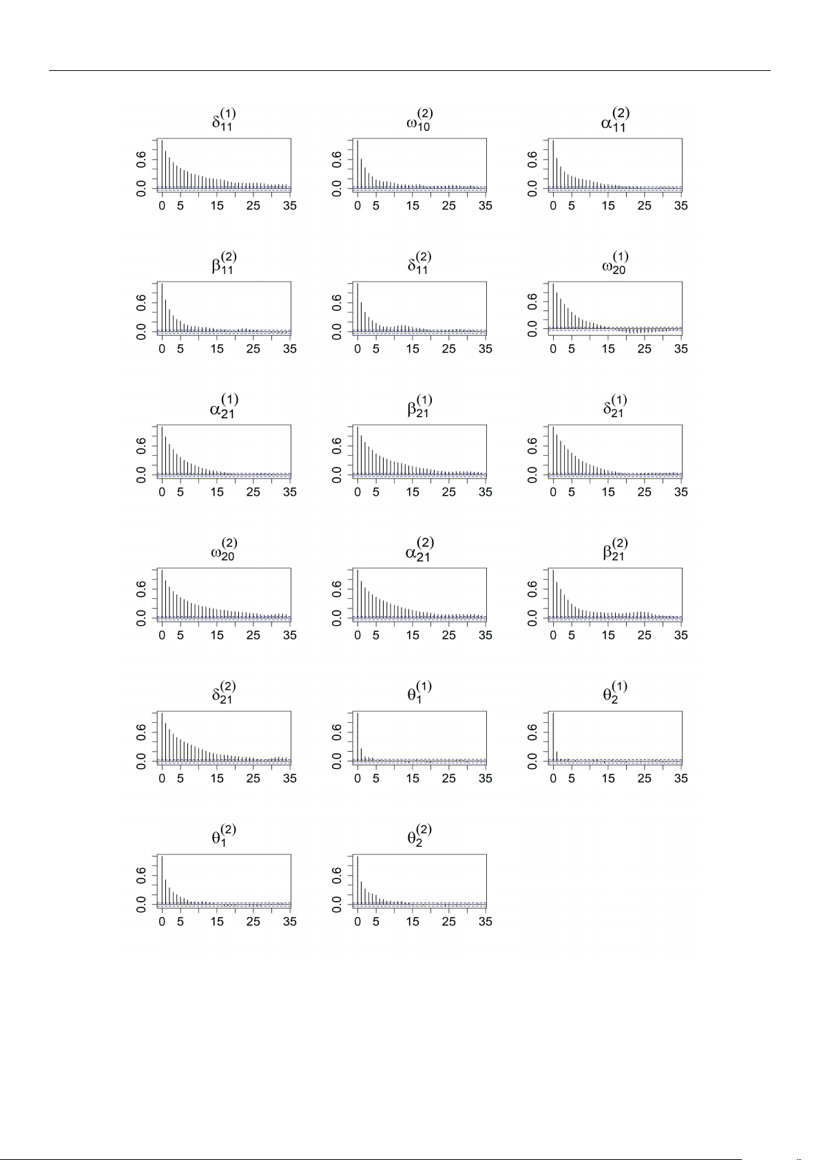
because the posterior probability for d = 1 is nearly equal to one. To check the convergence of
MCMC, we examine the ACF plots of all coefficients. For compactness, we present only the
autocorrelation function (ACF) plots based on Model 2, omitting the ACF plots of Model 1 to
conserve space. Figures 1 and 2 provide additional evidence supporting the convergence of the
MCMC algorithm. Based on these diagnostic checks, we conclude that the proposed models are
well suited for implementation within the Bayesian framework.
Table 1. Simulation results of the BHAR(1)–GJR–GARCH(1,1) model obtained from 200 replications. Parameter True Mean Med Std 2.5% 97.5% Coverage (1) ϕ −0.10 −0.1022 −0.1023 0.0280 −0.1573 −0.0472 94.00 10 (1) ϕ −0.10 −0.1014 −0.1015 0.0185 −0.1375 −0.0650 98.00 20 (1) ϕ 0.20 0.1992 0.1992 0.0482 0.1048 0.2936 95.50 11 (1) ϕ 0.25 0.2465 0.2465 0.0440 0.1602 0.3330 95.50 12 (1) ϕ 0.25 0.2510 0.2511 0.0215 0.2089 0.2932 96.00 21 (1) ϕ 0.30 0.2959 0.2960 0.0328 0.2312 0.3601 97.00 22 (2) ϕ −0.08 −0.0811 −0.0811 0.0119 −0.1045 −0.0579 94.50 10 (2) ϕ −0.15 −0.1512 −0.1512 0.0081 −0.1671 −0.1354 92.00 20 (2) ϕ 0.30 0.3005 0.3005 0.0347 0.2323 0.3688 95.50 11 (2) ϕ 0.35 0.3472 0.3472 0.0344 0.2797 0.4149 95.00 12 Entropy 2025, 27, 771 9 of 25 Table 1. Cont. Parameter True Mean Med Std 2.5% 97.5% Coverage (2) ϕ 0.35 0.3514 0.3514 0.0162 0.3197 0.3832 94.00 21 (2) ϕ 0.30 0.2972 0.2972 0.0234 0.2513 0.3432 95.00 22 rL −0.50 −0.4989 −0.4988 0.0184 −0.5334 −0.4640 94.50 rU 0.10 0.0885 0.0890 0.0324 0.0266 0.1503 92.50 ν1 8.00 9.1324 8.9642 1.4995 6.6907 12.5705 97.50 ν2 10.00 10.1588 9.9447 1.7664 7.3307 14.2193 98.50 (1) ρ 0.65 0.6460 0.6483 0.0323 0.5758 0.7021 97.50 (2) ρ 0.80 0.7990 0.7990 0.0295 0.7414 0.8572 95.50 d 1.00 1.0000 1.0000 0.0204 1.0000 1.0000 100.00 (1) ω 0.07 0.0782 0.0775 0.0144 0.0521 0.1088 89.50 10 (1) α 0.20 0.2139 0.2091 0.1148 0.0218 0.4385 100.00 11 (1) β 0.20 0.2191 0.2167 0.1143 0.0243 0.4388 100.00 11 (1) δ 0.40 0.3821 0.3819 0.0613 0.2620 0.5020 91.00 11 (2) ω 0.03 0.0349 0.0345 0.0073 0.0217 0.0506 91.00 10 (2) α 0.20 0.2147 0.2131 0.0356 0.1502 0.2899 96.50 11 (2) β 0.25 0.2792 0.2754 0.1150 0.0721 0.5080 97.00 11 (2) δ 0.55 0.5240 0.5248 0.0492 0.4245 0.6184 93.00 11 (1) ω 0.04 0.0382 0.0379 0.0068 0.0259 0.0524 93.00 20 (1) α 0.25 0.2458 0.2439 0.0682 0.1190 0.3837 97.00 21 (1) β 0.10 0.1262 0.1196 0.0694 0.0163 0.2754 97.50 21 (1) δ 0.40 0.3781 0.3781 0.0677 0.2450 0.5107 96.00 21 (2) ω 0.02 0.0218 0.0216 0.0039 0.0147 0.0298 94.00 20 (2) α 0.30 0.3063 0.3044 0.0441 0.2253 0.3971 97.00 21 (2) β 0.15 0.1830 0.1769 0.0830 0.0430 0.3542 95.00 21 (2) δ 0.40 0.3808 0.3809 0.0525 0.2781 0.4824 94.00 21 (1) θ 0.40 0.3915 0.3986 0.1819 0.0710 0.7004 97.00 1 (1) θ 0.10 0.1011 0.0968 0.0476 0.0258 0.1938 96.50 2 (2) θ 0.50 0.4615 0.4672 0.1083 0.2370 0.6571 96.50 1 (2) θ 0.20 0.2092 0.2065 0.0412 0.1364 0.2969 95.50 2
Table 2. Simulation results of the BHAR(1)–QGARCH(1,1) model obtained from 200 replications. Parameter True Mean Med Std 2.5% 97.5% Coverage (1) ϕ −0.10 −0.1003 −0.1002 0.0203 −0.1404 −0.0606 94.00 10 (1) ϕ −0.08 −0.0792 −0.0792 0.0153 −0.1093 −0.0493 93.50 20 (1) ϕ 0.32 0.3185 0.3186 0.0351 0.2494 0.3871 94.00 11 Entropy 2025, 27, 771 10 of 25 Table 2. Cont. Parameter True Mean Med Std 2.5% 97.5% Coverage (1) ϕ 0.30 0.2973 0.2972 0.0292 0.2401 0.3548 97.00 12 (1) ϕ 0.37 0.3717 0.3717 0.0217 0.3290 0.4143 94.50 21 (1) ϕ 0.35 0.3467 0.3467 0.0250 0.2976 0.3958 95.00 22 (2) ϕ −0.08 −0.0808 −0.0808 0.0108 −0.1021 −0.0595 96.50 10 (2) ϕ −0.08 −0.0802 −0.0802 0.0070 −0.0940 −0.0665 95.50 20 (2) ϕ 0.35 0.3427 0.3427 0.0394 0.2652 0.4197 94.00 11 (2) ϕ 0.30 0.3027 0.3027 0.0372 0.2295 0.3759 95.00 12 (2) ϕ 0.33 0.3290 0.3290 0.0183 0.2930 0.3647 94.00 21 (2) ϕ 0.37 0.3666 0.3667 0.0235 0.3204 0.4127 95.00 22 rL −0.45 −0.4501 −0.4503 0.0069 −0.4626 −0.4370 93.00 rU 0.10 0.0970 0.0973 0.0113 0.0750 0.1170 93.00 ν1 8.00 9.2129 9.0257 1.5569 6.7229 12.8309 93.50 ν2 10.00 10.2736 10.0551 1.8017 7.3914 14.4714 99.50 (1) ρ 0.50 0.4951 0.4994 0.0563 0.3723 0.5928 92.50 (2) ρ 0.85 0.8472 0.8479 0.0257 0.7948 0.8958 94.50 d 1.00 1.0000 1.0000 0.0152 1.0000 1.0000 100.00 (1) ω 0.07 0.0784 0.0778 0.0124 0.0557 0.1040 91.50 10 (1) α 0.20 0.2235 0.2213 0.0467 0.1386 0.3220 95.00 11 (1) β 0.10 0.1107 0.1098 0.0289 0.0566 0.1704 96.00 11 (1) δ 0.40 0.3613 0.3628 0.0832 0.1955 0.5205 95.50 11 (2) ω 0.03 0.0343 0.0340 0.0060 0.0234 0.0470 92.00 10 (2) α 0.30 0.3306 0.3282 0.0558 0.2291 0.4473 94.00 11 (2) β 0.10 0.1030 0.1032 0.0236 0.0555 0.1490 96.50 11 (2) δ 0.35 0.3289 0.3285 0.0527 0.2268 0.4339 94.00 11 (1) ω 0.04 0.0371 0.0369 0.0051 0.0276 0.0478 95.00 20 (1) α 0.40 0.4115 0.4095 0.0555 0.3089 0.5284 94.50 21 (1) β 0.05 0.0533 0.0525 0.0192 0.0180 0.0932 95.00 21 (1) δ 0.30 0.2855 0.2850 0.0618 0.1664 0.4087 95.00 21 (2) ω 0.02 0.0212 0.0211 0.0026 0.0163 0.0267 94.50 20 (2) α 0.30 0.3212 0.3197 0.0449 0.2387 0.4122 95.50 21 (2) β 0.10 0.1032 0.1031 0.0138 0.0767 0.1308 93.00 21 (2) δ 0.20 0.1904 0.1892 0.0410 0.1129 0.2733 96.00 21 (1) θ 0.40 0.3810 0.3847 0.1001 0.1753 0.5660 94.00 1 (1) θ 0.35 0.3582 0.3561 0.0563 0.2543 0.4744 96.00 2 (2) θ 0.55 0.5157 0.5244 0.0928 0.3104 0.6746 96.50 1 (2) θ 0.15 0.1573 0.1531 0.0427 0.0850 0.2535 98.00 2 Entropy 2025, 27, 771 11 of 25
Figure 1. ACF plots of after burn-in MCMC iterations for all parameters from the BHAR(1)–QGARCH(1,1) model. Entropy 2025, 27, 771 12 of 25
Figure 2. ACF plots of after burn-in MCMC iterations for all parameters from the BHAR(1)–QGARCH(1,1) model. 6. Emperical Study
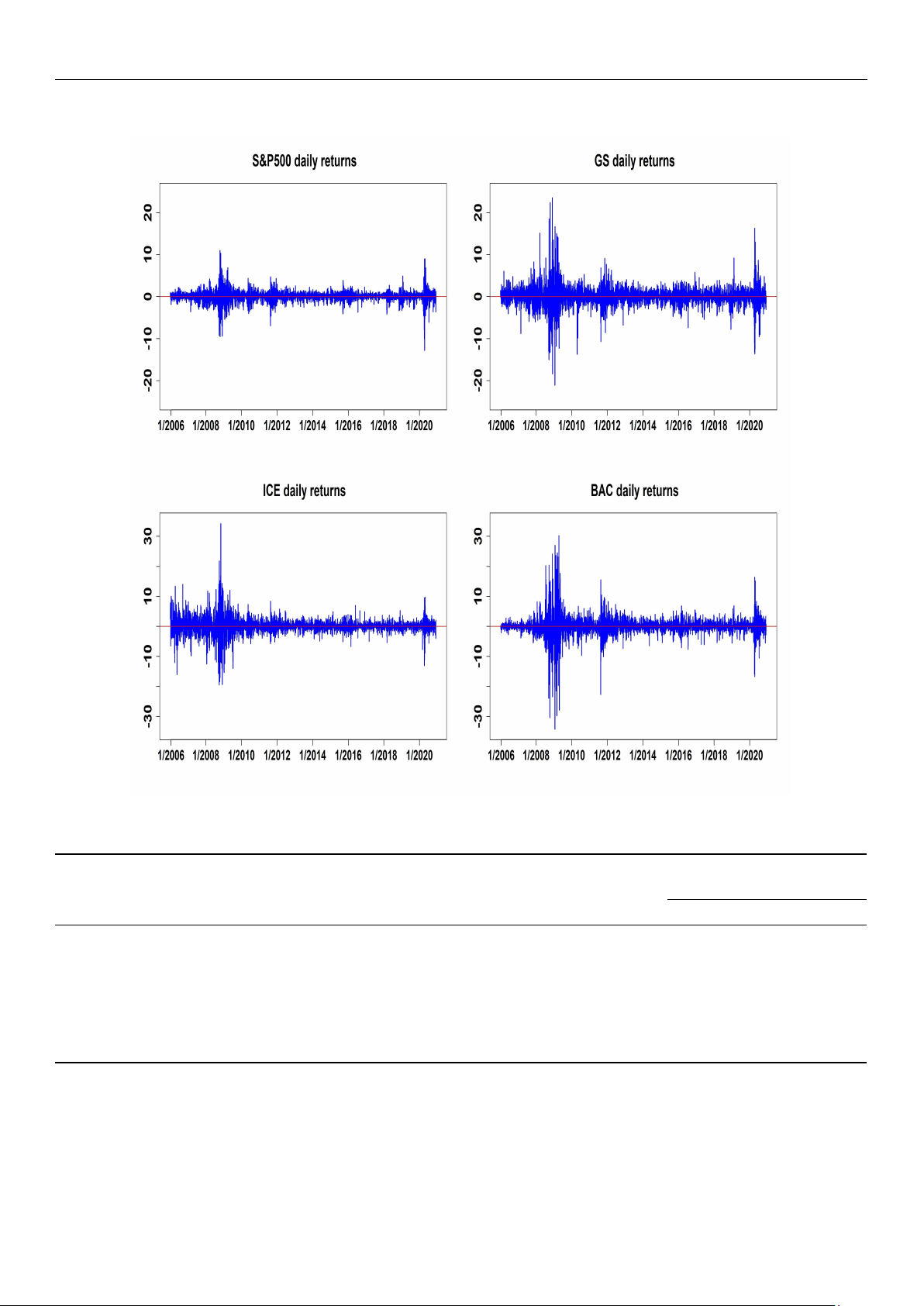
The empirical analysis in this study is based on the daily closing prices of four major
financial indices: the S&P500, Bank of America (BAC), Intercontinental Exchange (ICE), and Entropy 2025, 27, 771 13 of 25
Goldman Sachs (GS). The data span from 4 January 2006, to 30 December 2021, encompass-
ing a total of 4026 trading days. These data were retrieved from Yahoo Finance, a widely
recognized source for historical market data. To construct the return series, we compute the
continuously compounded returns (log-returns) using the formula yt = log(pt) − log(pt−1),
where pt denotes the asset’s closing price at time t.
Table 3 defines three target datasets: DS1 {S&P500, GS}, DS2 {S&P500, ICE}, and DS3
{S&P500, BAC}. It also presents the descriptive statistics of the corresponding return series,
along with the results of two multivariate normality tests: Mardia’s test and the Henze–
Zirkler test (see [23,24]). The return distributions are clearly skewed and have high kurtosis,
in particular, showing strong positive skewness. Due to the noticeable asymmetry and the
presence of heavy tails in the return data, we recommend using asymmetric models with fat-
tailed multivariate error distributions instead of models that assume multivariate normal
errors. Figure 3 presents the time series plot of daily returns for the selected financial assets.
As shown, the sample period spans several significant market events, notably the Global
Financial Crisis, which officially began on 15 September 2008, following the bankruptcy
of Lehman Brothers. For the purpose of estimation and out-of-sample evaluation, the
dataset is divided into two distinct sub-periods. The first segment, consisting of 3726 daily
observations, is used to estimate the model parameters. The remaining 300 observations
are reserved for out-of-sample forecasting and performance assessment.
This section’s hyper-parameters correspond to those in the simulation study. Tables 4–7
present a summary of the Bayesian estimates for three datasets for the BHAR(1)–GJR– (
GARCH(1,1) and the BHAR(1)–QGARCH(1,1) models. The significant value of 1) ϕ in 12
Tables 4 and 6 indicates that the performance of the previous day’s return of Goldman Sachs
stock has a considerable negative impact on the S&P 500’s returns in the lower regimes. We ( ( ( (
can see that the parameter estimates for 1) 2) 1) 2) ϕ , , , and are identical in both fitted 12 ϕ12 ϕ21 ϕ21
models when we look at datasets DS2 and DS3 in Tables 5 and 7. To assess the validity of
the proposed models, we further employ the Geweke convergence diagnostic (see [25]).
The p-values reported in Tables 8 and 9 suggest that the MCMC chains generated from
the models have converged. As there is no statistical evidence of non-convergence, we
conclude that the proposed models are appropriately specified and reliable for inference.
To evaluate the accuracy of the models using Value-at-Risk (VaR), we present VaR
forecasts along with the results of VaR backtesting at the 1% and 5% significance levels.
Specifically, Tables 10 and 11 report the p-values of the Unconditional Coverage (UC)
and Conditional Coverage (CC) tests for the two proposed models: bivariate HAR(1)–
GJR–GARCH(1,1) and HAR(1)–QGARCH(1,1) as well as the benchmark bivariate HAR(1)–
GARCH(1,1) model. When evaluating DS1, DS2, and DS3 across the three models, the
violation rates (VRate) for the S&P 500 tend to be significantly higher than the nominal
1% level, suggesting a slight underestimation of tail risk. In contrast, the VRates for Bank
of America (BAC), Intercontinental Exchange (ICE), and Goldman Sachs (GS) indicate a
tendency toward risk overestimation. Nevertheless, the backtesting results show that all
three models perform adequately as risk models. At the 5% significance level, both the
proposed models and the benchmark BHAR(1)–GARCH(1,1) model yield UC and CC test
p-values above 5%, indicating no statistical evidence of model misspecification. These
findings confirm that the proposed models deliver reliable and independent risk forecasts.
Figures 4 and 5 display the VaR forecasts based on the bivariate HAR(1)–GJR–GARCH(1,1)
and HAR(1)–QGARCH(1,1) models, which clearly show that the models are capable of
identifying volatility spikes in returns, despite infrequent violations of the forecast bounds.
To understand how well the proposed models can capture the expected shortfall
movement, we present the backtesting measures of the MES forecasts proposed by the
authors of [26] in Table 12. The model with the smallest values in the boxes is the best. Entropy 2025, 27, 771 14 of 25
These findings indicate that the proposed models are the best.
Figure 3. Time series plots of S&P 500, GS, ICE, and BAC daily returns.
Table 3. Summary statistics and multivariate normality tests. Data Mean Std Min Max Skewness Kurtosis MVN Tests ∗ (p-Value) Mardia Henze–Zirkler S&P500 0.033 1.256 −12.765 10.957 −0.568 16.737 GS 0.033 2.320 −21.022 23.482 0.188 18.086 ICE 0.075 2.578 −19.501 34.217 0.205 20.699 BAC 0.007 3.165 −34.206 30.210 −0.319 26.645 S&P500 vs. GS <0.001 <0.001 S&P 500 vs. ICE <0.001 <0.001 S&P 500 vs. BAC <0.001 <0.001
∗ : “MVN” stands for multivariate normality. Entropy 2025, 27, 771 15 of 25
Table 4. Estimation results, including posterior means, medians, standard deviations, and 95% Bayes
credible intervals of dataset DS1 {S&P 500, GS}, based on the BHAR(1)–GJR–GARCH(1,1) model. Parameter Mean Med Std 2.5% 97.5% (1) ϕ 0.0453 0.0454 0.0255 −0.0043 0.0967 10 (1) ϕ 0.0525 0.0538 0.0520 −0.0580 0.1502 20 (1) ϕ −0.0914 −0.0921 0.0375 −0.1624 −0.0205 11 (1) ϕ −0.0023 −0.0017 0.0178 −0.0371 0.0323 12 (1) ϕ −0.0274 −0.0284 0.0649 −0.1506 0.0972 21 (1) ϕ −0.0198 −0.0204 0.0353 −0.0880 0.0516 22 (2) ϕ 0.0408 0.0405 0.0137 0.0147 0.0680 10 (2) ϕ 0.0010 −0.0005 0.0340 −0.0648 0.0717 20 (2) ϕ 0.0054 0.0050 0.0283 −0.0500 0.0608 11 (2) ϕ −0.0265 −0.0267 0.0124 −0.0499 −0.0024 12 (2) ϕ 0.0339 0.0321 0.0575 −0.0792 0.1423 21 (2) ϕ −0.0421 −0.0411 0.0287 −0.1000 0.0111 22 rL −0.4935 −0.4744 0.0386 −0.5667 −0.4502 rU 0.6388 0.6497 0.0295 0.5541 0.6814 ν1 8.8291 8.7186 0.9056 7.2395 10.9435 ν2 7.4454 7.4002 0.7572 6.1675 9.1533 (1) ρ 0.8766 0.8765 0.0192 0.8393 0.9150 (2) ρ 0.6681 0.6699 0.0318 0.6014 0.7265 d 1.0000 1.0000 0.0318 1.0000 1.0000 (1) ω 0.0247 0.0243 0.0042 0.0170 0.0341 10 (1) α 0.0085 0.0082 0.0049 0.0009 0.0188 11 (1) β 0.1155 0.1153 0.0078 0.1007 0.1299 11 (1) δ 0.9285 0.9296 0.0073 0.9115 0.9389 11 (2) ω 0.0179 0.0178 0.0024 0.0135 0.0228 10 (2) α 0.0223 0.0222 0.0053 0.0117 0.0328 11 (2) β 0.2750 0.2747 0.0137 0.2483 0.3006 11 (2) δ 0.8189 0.8195 0.0114 0.7959 0.8404 11 (2) ω 0.0804 0.0796 0.0158 0.0525 0.1140 10 (2) α 0.0268 0.0266 0.0086 0.0101 0.0435 11 (2) β 0.0532 0.0528 0.0082 0.0370 0.0699 11 (2) δ 0.9353 0.9363 0.0112 0.9108 0.9549 11 (2) ω 0.0852 0.0850 0.0154 0.0565 0.1159 20 (2) α 0.0397 0.0396 0.0052 0.0298 0.0503 21 (2) β 0.0449 0.0452 0.0107 0.0240 0.0654 21 (2) δ 0.8482 0.8483 0.0139 0.8207 0.8737 21 (1) θ 0.8058 0.8060 0.0200 0.7676 0.8446 1 (1) θ 0.0325 0.0325 0.0030 0.0266 0.0383 2 (2) θ 0.8742 0.8744 0.0162 0.8428 0.9056 1 (2) θ 0.0428 0.0427 0.0032 0.0366 0.0491 2 Entropy 2025, 27, 771 16 of 25
Table 5. Estimation results, including posterior means and 95% Bayes credible intervals of datasets
DS2 and DS3, based on the BHAR(1)–GJR–GARCH(1,1) model. DS2 DS3 Parameter Mean 2.5% 97.5% Mean 2.5% 97.5% (1) ϕ 0.0871 0.0325 0.1398 0.0598 0.0081 0.1094 10 (1) ϕ 0.0742 −0.0073 0.1589 0.0017 −0.0931 0.0911 20 (1) ϕ −0.0331 −0.0915 0.0291 −0.1103 −0.1858 −0.0376 11 (1) ϕ −0.0299 −0.0563 −0.0035 0.0115 −0.0181 0.0395 12 (1) ϕ −0.1255 −0.2212 −0.0305 −0.2095 −0.3419 −0.0754 21 (1) ϕ −0.0393 −0.0947 0.0168 0.0721 0.0058 0.1372 22 (2) ϕ 0.0514 0.0218 0.0787 0.0471 0.0203 0.0728 10 (2) ϕ 0.0270 −0.0346 0.0860 0.0342 −0.0222 0.0882 20 (2) ϕ −0.0372 −0.0857 0.0130 −0.0299 −0.0829 0.0255 11 (2) ϕ −0.0094 −0.0241 0.0043 −0.0155 −0.0336 0.0018 12 (2) ϕ −0.0181 −0.1160 0.0778 −0.1706 −0.2781 −0.0684 21 (2) ϕ −0.0553 −0.1000 −0.0091 0.0213 −0.0304 0.0708 22 rL −0.5351 −0.5778 −0.4536 −0.5601 −0.5769 −0.5315 rU 0.6238 0.5814 0.6569 0.6208 0.5852 0.6668 ν1 6.8541 5.6768 8.3212 8.9290 7.2431 10.8435 ν2 5.1780 4.4976 6.0264 6.1178 5.2628 7.0598 (1) ρ 0.8877 0.8006 0.9790 0.8202 0.7953 0.8431 (2) ρ 0.2767 0.1298 0.3908 0.5443 0.4328 0.6347 d 1.0000 1.0000 1.0000 1.0000 1.0000 1.0000 (1) ω 0.0210 0.0145 0.0312 0.0276 0.0174 0.0395 10 (1) α 0.0115 0.0018 0.0233 0.0148 0.0017 0.0302 11 (1) β 0.0989 0.0840 0.1132 0.1115 0.0978 0.1253 11 (1) δ 0.9337 0.9178 0.9441 0.9221 0.9013 0.9384 11 (2) ω 0.0142 0.0100 0.0188 0.0169 0.0125 0.0216 10 (2) α 0.0164 0.0040 0.0305 0.0224 0.0124 0.0336 11 (2) β 0.2234 0.1814 0.2657 0.2727 0.2426 0.2999 11 (2) δ 0.8368 0.8118 0.8592 0.8261 0.8047 0.8456 11 (1) ω 0.0424 0.0202 0.0703 0.1096 0.0734 0.1484 20 (1) α 0.0313 0.0118 0.0512 0.0653 0.0401 0.0927 21 (1) β 0.0481 0.0309 0.0654 0.0472 0.0247 0.0692 21 (1) δ 0.9356 0.9073 0.9562 0.8704 0.8372 0.8974 21 (2) ω 0.0366 0.0206 0.0550 0.0165 0.0020 0.0358 20 (2) α 0.0533 0.0424 0.0653 0.0540 0.0423 0.0667 21 (2) β 0.0381 0.0242 0.0525 0.0996 0.0756 0.1234 21 (2) δ 0.8506 0.8217 0.8776 0.8644 0.8381 0.8857 21 (1) θ 0.8311 0.7798 0.8711 0.3327 0.2778 0.3865 1 (1) θ 0.0599 0.0521 0.0683 0.1297 0.1155 0.1438 2 (2) θ 0.9266 0.9114 0.9419 0.9137 0.8977 0.9292 1 (2) θ 0.0254 0.0211 0.0297 0.0340 0.0294 0.0384 2 Entropy 2025, 27, 771 17 of 25
Table 6. Results of estimation of the BHAR(1)–QGARCH(1,1) model are shown, including posterior
means, medians, standard deviations, and 95% Bayes credible intervals of the dataset DS1. Parameter Mean Med Std 2.5% 97.5% (1) ϕ 0.0139 0.0128 0.0328 −0.0493 0.0796 10 (1) ϕ −0.0248 −0.0279 0.0584 −0.1333 0.0933 20 (1) ϕ −0.0638 −0.0663 0.0454 −0.1448 0.0290 11 (1) ϕ −0.0370 −0.0370 0.0170 −0.0699 −0.0039 12 (1) ϕ −0.0100 −0.0138 0.0797 −0.1648 0.1542 21 (1) ϕ −0.0657 −0.0651 0.0375 −0.1386 0.0053 22 (2) ϕ 0.0338 0.0336 0.0153 0.0052 0.0658 10 (2) ϕ 0.0179 0.0191 0.0347 −0.0535 0.0869 20 (2) ϕ −0.0217 −0.0224 0.0298 −0.0792 0.0379 11 (2) ϕ −0.0050 −0.0048 0.0122 −0.0290 0.0201 12 (2) ϕ −0.0261 −0.0244 0.0592 −0.1475 0.0836 21 (2) ϕ −0.0072 −0.0071 0.0274 −0.0617 0.0481 22 rL −0.1680 −0.1595 0.0222 −0.2108 −0.1405 rU 0.0179 −0.0013 0.0449 −0.0329 0.1243 ν1 8.7278 8.6580 0.9039 7.0614 10.6549 ν2 7.3638 7.3355 0.6199 6.1993 8.6153 (1) ρ 0.8502 0.8501 0.0134 0.8239 0.8759 (2) ρ 0.2581 0.3011 0.2326 −0.3197 0.5698 d 1.0000 1.0000 0.2326 1.0000 1.0000 (1) ω 0.0817 0.0813 0.0043 0.0742 0.0902 10 (1) α 0.1243 0.1244 0.0087 0.1066 0.1415 11 (1) β 0.0092 0.0093 0.0032 0.0026 0.0153 11 (1) δ 0.8724 0.8728 0.0096 0.8534 0.8916 11 (2) ω 0.0036 0.0035 0.0014 0.0009 0.0065 10 (2) α 0.0201 0.0202 0.0050 0.0106 0.0300 11 (2) β 0.0037 0.0033 0.0025 0.0002 0.0093 11 (2) δ 0.8448 0.8448 0.0102 0.8237 0.8635 11 (1) ω 0.1986 0.1975 0.0243 0.1490 0.2492 20 (1) α 0.0886 0.0880 0.0086 0.0732 0.1066 21 (1) β 0.0310 0.0309 0.0124 0.0083 0.0555 21 (1) δ 0.9002 0.9015 0.0140 0.8686 0.9248 21 (2) ω 0.0435 0.0425 0.0146 0.0150 0.0726 20 (2) α 0.0422 0.0420 0.0058 0.0314 0.0536 21 (2) β 0.0123 0.0123 0.0052 0.0029 0.0232 21 (2) δ 0.8589 0.8595 0.0133 0.8316 0.8816 21 (1) θ 0.6106 0.6104 0.0155 0.5806 0.6422 1 (1) θ 0.0407 0.0407 0.0036 0.0338 0.0477 2 (2) θ 0.9163 0.9179 0.0158 0.8818 0.9403 1 (2) θ 0.0503 0.0504 0.0046 0.0425 0.0584 2 Entropy 2025, 27, 771 18 of 25
Table 7. Estimation results are shown, including posterior means and 95% Bayes credible intervals of
datasets DS1, DS2, and DS3, based on the BHAR(1)–QGARCH(1,1) model. DS1 DS2 DS3 Parameter Mean 2.5% 97.5% Mean 2.5% 97.5% Mean 2.5% 97.5% (1) ϕ 0.0139 0.0328 −0.0493 0.0476 −0.0161 0.1136 0.0753 0.0219 0.1301 10 (1) ϕ −0.0248 0.0584 −0.1333 0.0654 −0.0425 0.1699 0.0267 −0.0725 0.1215 20 (1) ϕ −0.0638 0.0454 0.0454 −0.0579 −0.1326 0.0212 −0.1049 −0.1784 −0.0299 11 (1) ϕ −0.0370 0.0170 0.0170 −0.0376 −0.0600 −0.0135 0.0060 −0.0227 0.0332 12 (1) ϕ −0.0100 0.0797 0.0797 −0.1247 −0.2361 −0.0108 −0.1902 −0.3188 −0.0611 21 (1) ϕ −0.0657 0.0375 0.0375 −0.0581 −0.1167 0.0016 0.0550 −0.0102 0.1181 22 (2) ϕ 0.0338 0.0153 0.0153 0.0413 0.0084 0.0738 0.0418 0.0107 0.0692 10 (2) ϕ 0.0179 0.0347 0.0347 0.0046 −0.0635 0.0696 0.0309 −0.0239 0.0867 20 (2) ϕ −0.0217 0.0298 0.0298 −0.0236 −0.0837 0.0270 −0.0236 −0.0732 0.0309 11 (2) ϕ −0.0050 0.0122 0.0122 −0.0063 −0.0226 0.0099 −0.0117 −0.0292 0.0059 12 (2) ϕ −0.0261 0.0592 0.0592 0.0158 −0.0893 0.1169 −0.1659 −0.2692 −0.0598 21 (2) ϕ −0.0072 0.0274 0.0274 −0.0475 −0.0951 −0.0029 0.0314 −0.0202 0.0814 22 rL −0.1680 0.0222 0.0222 −0.2019 −0.2123 −0.1811 −0.5473 −0.5747 −0.4611 rU 0.0179 0.0449 0.0449 0.0524 −0.0385 0.1507 0.6111 0.5527 0.6559 ν1 8.7278 0.9039 0.9039 6.8073 5.5809 8.3232 8.9350 7.3051 10.8176 ν2 7.3638 0.6199 0.6199 5.2143 4.5484 5.9952 6.0211 5.1460 7.0315 (1) ρ 0.8502 0.0134 0.0134 0.9172 0.8269 0.9912 0.8109 0.7864 0.8350 (2) ρ 0.2581 0.2326 0.2326 −0.4946 −0.9541 0.0104 0.4795 0.0228 0.6653 d 1.0000 0.2326 0.2326 1.0000 1.0000 1.0000 1.0000 1.0000 1.0000 (1) ω 0.0817 0.0043 0.0043 0.0604 0.0510 0.0712 0.0486 0.0357 0.0637 10 (1) α 0.1243 0.0087 0.0087 0.1046 0.0899 0.1219 0.1214 0.1067 0.1380 11 (1) β 0.0092 0.0032 0.0032 0.0077 0.0006 0.0159 0.0077 0.0003 0.0228 11 (1) δ 0.8724 0.0096 0.0096 0.8916 0.8704 0.9085 0.8748 0.8573 0.8916 11 (2) ω 0.0036 0.0014 0.0014 0.0033 0.0007 0.0067 0.0194 0.0144 0.0249 10 (2) α 0.0201 0.0050 0.0050 0.0159 0.0050 0.0275 0.0318 0.0186 0.0472 11 (2) β 0.0037 0.0025 0.0025 0.0035 0.0005 0.0066 0.0025 0.0003 0.0049 11 (2) δ 0.8448 0.0102 0.0102 0.8628 0.8411 0.8832 0.8427 0.8174 0.8655 11 (1) ω 0.1986 0.0243 0.0243 0.0685 0.0457 0.0938 0.1229 0.0857 0.1593 20 (1) α 0.0886 0.0086 0.0086 0.0742 0.0578 0.0945 0.1115 0.0883 0.1343 21 (1) β 0.0310 0.0124 0.0124 0.0127 0.0032 0.0231 0.0149 0.0031 0.0279 21 (1) δ 0.9002 0.0140 0.0140 0.9164 0.8854 0.9391 0.8462 0.8143 0.8775 21 (2) ω 0.0435 0.0146 0.0146 0.0214 0.0037 0.0417 0.0176 0.0025 0.0381 20 (2) α 0.0422 0.0058 0.0058 0.0539 0.0424 0.0664 0.0650 0.0549 0.0769 21 (2) β 0.0123 0.0052 0.0052 0.0058 0.0006 0.0122 0.0061 0.0012 0.0119 21 (2) δ 0.8589 0.0133 0.0133 0.8709 0.8462 0.8923 0.8766 0.8514 0.8970 21 (1) θ 0.6106 0.0155 0.0155 0.8121 0.7590 0.8588 0.3322 0.2221 0.4398 1 (1) θ 0.0407 0.0036 0.0036 0.0636 0.0492 0.0774 0.1214 0.0944 0.1499 2 (2) θ 0.9163 0.0158 0.0158 0.9664 0.9447 0.9801 0.9279 0.8839 0.9620 1 (2) θ 0.0503 0.0046 0.0046 0.0124 0.0037 0.0221 0.0340 0.0226 0.0447 2 Entropy 2025, 27, 771 19 of 25
Table 8. Geweke diagnostic of all parameters for DS1, DS2, and DS3 based on the BHAR(1)–GJR– GARCH(1,1) model. DS1 DS2 DS3 Parameter Statistic p-Value Statistic p-Value Statistic p-Value (1) ϕ −0.0597 0.9524 −0.8079 0.4192 −0.0636 0.9493 10 (1) ϕ −0.1791 0.8579 −0.3346 0.7379 −0.0162 0.9870 20 (1) ϕ 1.3573 0.1747 −1.5891 0.1120 −0.2181 0.8274 11 (1) ϕ 0.7764 0.4375 1.7514 0.0799 −0.4235 0.6720 12 (1) ϕ 0.5771 0.5639 −2.2308 0.0257 −0.0380 0.9697 21 (1) ϕ 0.6501 0.5156 1.8316 0.0670 −0.7052 0.4807 22 (2) ϕ 1.8243 0.0681 0.4597 0.6457 −0.7424 0.4579 10 (2) ϕ 1.5591 0.1190 1.8774 0.0605 −0.6209 0.5346 20 (2) ϕ 0.1958 0.8448 −0.6016 0.5474 −0.9727 0.3307 11 (2) ϕ −1.1547 0.2482 1.5224 0.1279 0.3103 0.7564 12 (2) ϕ 1.0562 0.2909 −1.2477 0.2121 −0.5624 0.5738 21 (2) ϕ −1.9255 0.0542 −0.6378 0.5236 −0.0487 0.9611 22 rL −1.1629 0.2449 −2.8326 0.0046 1.8200 0.0688 rU −0.2210 0.8251 0.2319 0.8166 1.0950 0.2735 ν1 −1.1139 0.2653 −0.9501 0.3421 0.9806 0.3268 ν2 −1.6291 0.1033 0.0019 0.9985 0.1521 0.8791 (1) ρ −0.7965 0.4258 1.1421 0.2534 −1.6976 0.0896 (2) ρ 1.2195 0.2227 −0.9170 0.3591 1.2624 0.2068 (1) ω −0.9039 0.3660 −0.3661 0.7143 0.0221 0.9824 10 (1) α 0.9563 0.3389 −1.2333 0.2174 0.1894 0.8498 11 (1) β −1.3752 0.1691 1.0816 0.2794 1.2501 0.2113 11 (1) δ −0.0239 0.9809 −0.4108 0.6813 −0.8739 0.3822 11 (2) ω 0.2948 0.7682 −0.4945 0.6209 0.4263 0.6699 10 (2) α 0.0896 0.9286 −2.0540 0.0400 −0.2839 0.7765 11 (2) β −0.0769 0.9387 0.9074 0.3642 1.8353 0.0665 11 (2) δ −0.4204 0.6742 −0.8867 0.3753 0.3284 0.7426 11 (1) ω 1.6858 0.0918 0.6269 0.5307 −1.2515 0.2107 20 (1) α −0.8687 0.3850 1.4275 0.1534 −1.1246 0.2608 21 (1) β 1.2312 0.2182 −0.6642 0.5066 0.7641 0.4448 21 (1) δ −1.3606 0.1736 −0.5054 0.6133 0.5095 0.6104 21 (2) ω 0.0002 0.9999 0.4037 0.6864 −0.1893 0.8499 20 (2) α −1.6979 0.0895 0.6527 0.5139 −0.6733 0.5008 21 (2) β 1.2623 0.2068 1.0262 0.3048 −0.4108 0.6812 21 (2) δ 0.0031 0.9975 −1.2335 0.2174 1.0696 0.2848 21 (1) θ −1.0077 0.3136 0.2864 0.7746 −0.2729 0.7850 1 (1) θ 0.2581 0.7963 −0.6037 0.5460 0.1467 0.8834 2 (2) θ 0.6031 0.5465 0.4883 0.6253 −1.0627 0.2879 1 (2) θ 0.4767 0.6336 −1.0663 0.2863 1.9815 0.0475 2 Entropy 2025, 27, 771 20 of 25
Table 9. Geweke diagnostic of all parameters for DS1, DS2, and DS3 based on the BHAR(1)– QGARCH(1,1) model. DS1 DS2 DS3 Parameter Statistic p-Value Statistic p-Value Statistic p-Value (1) ϕ −0.2382 0.8117 0.8946 0.3710 0.4246 0.6711 10 (1) ϕ −0.5397 0.5894 0.4807 0.6308 0.2105 0.8332 20 (1) ϕ −0.3970 0.6914 1.0016 0.3165 0.4172 0.6765 11 (1) ϕ 0.3031 0.7618 −0.4317 0.6659 −0.0186 0.9852 12 (1) ϕ −0.9387 0.3479 0.0066 0.9947 0.6520 0.5144 21 (1) ϕ 0.6678 0.5043 0.3082 0.7579 −0.0690 0.9450 22 (2) ϕ −0.8183 0.4132 −1.0205 0.3075 1.2391 0.2153 10 (2) ϕ −1.3403 0.1802 −0.6150 0.5386 0.8368 0.4027 20 (2) ϕ 0.9480 0.3431 0.5433 0.5869 −0.8564 0.3918 11 (2) ϕ 0.3792 0.7045 0.1913 0.8483 −0.3520 0.7248 12 (2) ϕ 1.0261 0.3048 −0.1062 0.9154 0.2221 0.8242 21 (2) ϕ −0.1441 0.8854 0.2735 0.7845 −0.6287 0.5295 22 rL 0.1648 0.8691 −2.0563 0.0398 0.5816 0.5608 rU −0.6512 0.5149 0.4157 0.6777 −0.8724 0.3830 ν1 −0.0228 0.9818 −0.6572 0.5110 −0.1623 0.8711 ν2 0.2329 0.8159 −0.3896 0.6969 −0.7089 0.4784 (1) ρ −0.6398 0.5223 0.4073 0.6838 −0.3435 0.7312 (2) ρ 0.5406 0.5888 0.3116 0.7554 0.3015 0.7630 (1) ω −0.2259 0.8213 0.5642 0.5726 −1.3067 0.1913 10 (1) α 0.1495 0.8811 0.8659 0.3866 0.5879 0.5566 11 (1) β 0.9298 0.3525 −0.2060 0.8368 −1.9950 0.0460 11 (1) δ −0.1064 0.9153 −0.6188 0.5360 −0.2741 0.7840 11 (2) ω −0.2187 0.8269 0.0908 0.9277 0.6828 0.4947 10 (2) α −0.6417 0.5211 0.0376 0.9700 0.8227 0.4107 11 (2) β 0.2499 0.8027 1.5369 0.1243 0.7921 0.4283 11 (2) δ 0.5778 0.5634 −0.9276 0.3536 −1.1088 0.2675 11 (1) ω 0.0092 0.9927 −0.4402 0.6598 0.2285 0.8193 20 (1) α 0.8557 0.3922 −1.3612 0.1734 0.3195 0.7494 21 (1) β −1.1870 0.2352 −0.9613 0.3364 0.8448 0.3982 21 (1) δ −0.7819 0.4343 1.3219 0.1862 −0.0380 0.9697 21 (2) ω −0.9052 0.3654 −0.1715 0.8638 1.4796 0.1390 20 (2) α −0.8971 0.3697 0.0572 0.9544 0.3983 0.6904 21 (2) β 1.0325 0.3018 −0.1454 0.8844 −0.6278 0.5301 21 (2) δ 0.7220 0.4703 0.1081 0.9139 −0.9705 0.3318 21 (1) θ −0.1814 0.8561 0.5558 0.5783 0.3816 0.7028 1 (1) θ 2.2145 0.0268 −0.3652 0.7150 −1.0568 0.2906 2 (2) θ −0.9347 0.3500 −0.4136 0.6792 −0.0394 0.9686 1 (2) θ 0.6555 0.5121 1.1169 0.2640 −1.2179 0.2233 2
Tài liệu liên quan:
-

Ung dung game hoa trong cac chien dich MKT
27 14 -

Bao cao Chi so TMDT Viet Nam 2025
30 15 -

Thông tư quy định về việc phân quyền, phân cấp và phân định thẩm quyền quản lý nhà nước về giáo dục cho chính quyền địa phương
32 16 -

Nghị quyết về phát huy các giá trị di sản văn hóa gắn với phát triên du lịch bền vững tỉnh Khánh Hòa đến năm 2025, định hướng đến năm 2030
34 17 -

Quyết định phê duyệt Chiến lược phát triển du lịch Việt Nam đến năm 2030
21 11