Giáo trình Giải tích hàm một biến số | Trường Đại học Bách khoa - Đại học Quốc gia Thành phố Hồ Chí Minh
Giáo trình Giải tích hàm một biến số | Trường Đại học Bách khoa - Đại học Quốc gia Thành phố Hồ Chí Minh. Tài liệu được sưu tầm giúp bạn tham khảo, ôn tập và đạt kết quả cao. Mời bạn đọc đón xem.
Môn: Giải tích 44 tài liệu
Trường: Trường Đại học Bách khoa - Đại học Quốc gia Thành phố Hồ Chí Minh 721 tài liệu
Tác giả:


Preview text:
TS. NGUYỄN ĐỨC HẬU 350 ■ CHAPTER 5 INTEGRALS
The width of the interval 关a, b兴 is b ,
a so the width of each of the n strips is
x 苷 b a n
These strips divide the interval [a, b] into n subintervals
关x0, x1兴, 关x1, x2兴, 关x2, x3兴, . . . , 关xn1, xn兴 GIẢI
where x0 苷 a TÍCH and xn 苷 . b HÀM MỘT BIẾN
The right-hand endpoints of the subintervals are SỐ
x1 苷 a x, x2 苷 a 2 x, x3 苷 a 3 x, . . .
(Dùng cho sinh viên Trường Đại học Thủy lợi)
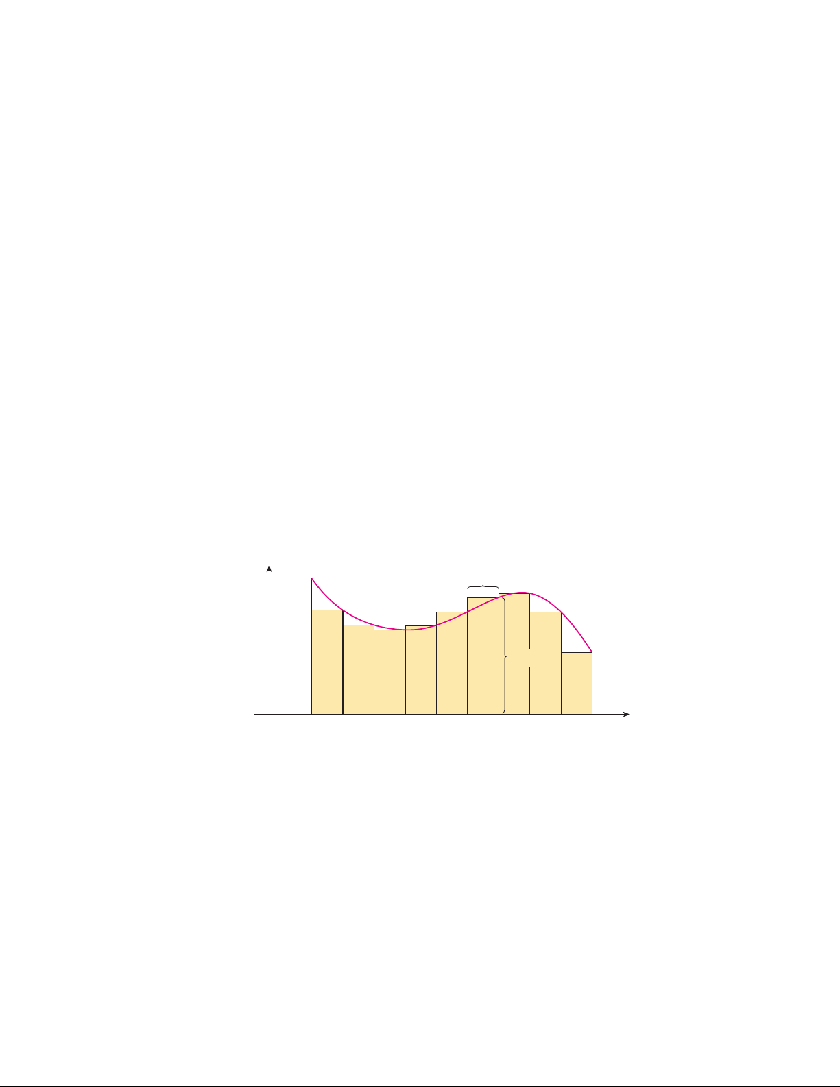
Let’s approximate the ith strip Si by a rectangle with width x and height f 共xi , 兲
which is the value of f at the right-hand endpoint (see Figure 11). Then the area of the th rectangle is i
f 共xi兲 x. What we think of intuitively as the area of S is approximated
by the sum of the areas of these rectangles, which is
Rn 苷 f 共x1兲 x f 共x2兲 x f 共xn兲 x y Îx f(x ) i 0 a ⁄ ¤ ‹ x b i-1 xi x FIGURE 11
Figure 12 shows this approximation for n 苷 ,
2 4, 8, and 12. Notice that this
approximation appears to become better and better as the number of strips increases,
that is, as n l . Therefore, we define the area A of the region S in the following way.
2 Definition The area A of the region S that lies under the graph of the
continuous function f is the limit of the sum of the areas of approximating rectangles: Hà nội 2013
A 苷 lim Rn 苷 lim 关 f 共x1兲 x f 共x2兲 x f 共xn兲 x兴 n l n l y y y y 0 a ⁄ b x 0 a ⁄ ¤ ‹ b x 0 a b x 0 a b x (a) n=2 (b) n=4 (c) n=8 (d) n=12 FIGURE 12 Mục lục Chương 1.
GIỚI HẠN VÀ TÍNH LIÊN TỤC CỦA HÀM SỐ 4
1.1. Hàm số một biến số
. . . . . . . . . . . . . . . . . . . . . . . . . . . 4
1.2. Giới hạn của dãy số thực
. . . . . . . . . . . . . . . . . . . . . . . . 9
1.3. Giới hạn của hàm số thực . . . . . . . . . . . . . . . . . . . . . . . . 10
1.4. Hàm số liên tục . . . . . . . . . . . . . . . . . . . . . . . . . . . . . . 19 Chương 2.
PHÉP TÍNH VI PHÂN CỦA HÀM MỘT BIẾN SỐ 22
2.1. Tiếp tuyến và vận tốc . . . . . . . . . . . . . . . . . . . . . . . . . . 22 2.2. Đạo hàm
. . . . . . . . . . . . . . . . . . . . . . . . . . . . . . . . . 23
2.3. Vi phân . . . . . . . . . . . . . . . . . . . . . . . . . . . . . . . . . . 26
2.4. Đạo hàm và vi phân cấp cao
. . . . . . . . . . . . . . . . . . . . . . 27
2.5. Các định lí về hàm khả vi . . . . . . . . . . . . . . . . . . . . . . . . 30 2.6. Quy tắc Lô-pi-tan
. . . . . . . . . . . . . . . . . . . . . . . . . . . . 32
2.7. Khảo sát hàm số . . . . . . . . . . . . . . . . . . . . . . . . . . . . . 36
2.8. Đường cong cho bởi phương trình tham số . . . . . . . . . . . . . . . 41
2.9. Đường cong trong tọa độ cực . . . . . . . . . . . . . . . . . . . . . . 44 Chương 3. TÍCH PHÂN 50
3.1. Tích phân bất định . . . . . . . . . . . . . . . . . . . . . . . . . . . . 50
3.2. Các phương pháp tính tích phân bất định . . . . . . . . . . . . . . . 51
3.3. Tích phân bất định của một vài lớp hàm . . . . . . . . . . . . . . . . 58
3.4. Tích phân xác định . . . . . . . . . . . . . . . . . . . . . . . . . . . . 69
3.5. Tích phân suy rộng với cận vô hạn . . . . . . . . . . . . . . . . . . . 76
3.6. Tích phân suy rộng của hàm không bị chặn . . . . . . . . . . . . . . 80
3.7. Một số ứng dụng của tích phân xác định . . . . . . . . . . . . . . . . 84
3.7.1. Tính diện tích hình phẳng . . . . . . . . . . . . . . . . . . . . 84
3.7.2. Tính độ dài cung . . . . . . . . . . . . . . . . . . . . . . . . . 89
3.7.3. Tính thể tích . . . . . . . . . . . . . . . . . . . . . . . . . . . 91
3.7.4. Tính diện tích của mặt tròn xoay . . . . . . . . . . . . . . . . 96 2 Chương 4. CHUỖI 99
4.1. Chuỗi số . . . . . . . . . . . . . . . . . . . . . . . . . . . . . . . . . . 99
4.2. Chuỗi số dương . . . . . . . . . . . . . . . . . . . . . . . . . . . . . . 101
4.3. Chuỗi số đan dấu . . . . . . . . . . . . . . . . . . . . . . . . . . . . . 105
4.4. Chuỗi số có dấu bất kì . . . . . . . . . . . . . . . . . . . . . . . . . . 106 4.5. Chuỗi hàm
. . . . . . . . . . . . . . . . . . . . . . . . . . . . . . . . 108
4.6. Chuỗi lũy thừa . . . . . . . . . . . . . . . . . . . . . . . . . . . . . . 110
4.7. Chuỗi Taylor và chuỗi Maclaurin . . . . . . . . . . . . . . . . . . . . 114
4.8. Chuỗi Fourier . . . . . . . . . . . . . . . . . . . . . . . . . . . . . . . 119 TS. NGUYỄN ĐỨC HẬU
http://nguyenduchau.wordpress.com Lời nói đầu
Bài giảng này được dành cho sinh viên của Trường Đại học Thủy lợi khi học môn
Toán 1 (Giải tích hàm một biến số). TS. NGUYỄN ĐỨC HẬU
http://nguyenduchau.wordpress.com 12 ■
CHAPTER 1 FUNCTIONS AND MODELS
A function f is a rule that assigns to each element x in a set A exactly one
element, called f 共x兲, in a set B.
We usually consider functions for which the sets A and B are sets of real numbers.
The set A is called the domain of the function. The number f 共x兲 is the value of f
at x and is read “ f of x.” The range of f is the set of all possible values of f 共x兲 as x
varies throughout the domain. A symbol that represents an arbitrary number in the
domain of a function f is called an independent variable. A symbol that represents 12 ■
CHAPTER 1 FUNCTIONS AND MODELS
a number in the range of f is called a dependent variable. In Example A, for
instance, r is the independent variable and A is the dependent variable.
It’s helpful to think of a function as a machine (see Figure 2). If x is in the domain
A function f is a rule that assigns to each element x in a set A exactly one x f ƒ (input) Chương (output) 1
of the function f, then when x enters the machine, it’s accepted as an input and the
element, called f 共x兲, in a set B.
machine produces an output f 共x兲 according to the rule of the function. Thus, we can FIGURE 2
think of the domain as the set of all possible inputs and the range as the set of all pos- GIỚI
Machine diagram for a function ƒ HẠN sible outputs. VÀ TÍNH
The preprogrammed functions in a calculator are good e LIÊN
We usually consider functions for which the sets A and B are sets of real numbers.
The set A is called the domain of the function. The number f 共x兲 is the value of f xamples of a function as a
at x and is read “ f of x.” The range of f is the set of all possible values of f 共x兲 as x
machine. For example, the square root key on your calculator is such a function. You
varies throughout the domain. A symbol that represents an arbitrary number in the TỤC CỦA press the key labeled sHÀM (or sx ) x ⬍ 0 x
domain of this function; that is, x SỐ
and enter the input x. If , then is not in the
domain of a function f is called an independent variable. A symbol that represents
is not an acceptable input, and the calculator will
a number in the range of f is called a dependent variable. In Example A, for x ƒ
indicate an error. If x 艌 0, then an approximation to sx will appear in the display.
instance, r is the independent variable and A is the dependent variable.
Thus, the sx key on your calculator is not quite the same as the exact mathematical
It’s helpful to think of a function as a machine (see Figure 2). If x is in the domain x f ƒ a f(a) function defined f by
f 共x兲 苷 sx. (input) (output)
of the function f, then when x enters the machine, it’s accepted as an input and the
machine produces an output f
Another way to picture a function is by an arrow diagram as in Figure 3. Each
共x兲 according to the rule of the function. Thus, we can FIGURE 2
think of the domain as the set of all possible inputs and the range as the set of all pos-
arrow connects an element of A to an element of .
B The arrow indicates that f 共x兲 is 1.1. Hàm số một biến số
Machine diagram for a function ƒ sible outputs. f
associated with x, f 共a兲 is associated with a, and so on. A B
The preprogrammed functions in a calculator are good examples of a function as a
The most common method for visualizing a function is its graph. If f is a function
machine. For example, the square root key on your calculator is such a function. You FIGURE 3 Định nghĩa 1.1 Cho with domain A , A ⊂ R. then its Hàm
graph số f xác định trên is the set of ordered pairs A
press the key labeled s (or sx ) and enter the input x. If x ⬍ 0, then x is not in the Arrow diagram for ƒ
là một quy tắc sao cho nó tác động vào một phần tử x bất
domain of this function; that is, x is not an acceptable input, and the calculator will
兵共x, f 共x兲兲 ⱍx 僆 A其
kì của A sẽ tạo thành một và chỉ một phần tử y của x ƒ
indicate an error. If x 艌 0, then an approximation to sx will appear in the display. R. Kí
Thus, the sx key on your calculator is not quite the same as the exact mathematical
hiệu f : A → R, x 7→ y = f (x). a f(a)
(Notice that these are input-output pairs.) In other words, the graph of f consists of all function defined f by
f 共x兲 苷 sx. A được gọi là tập points 共 nguồn x, y兲 hay tập xác định của
in the coordinate plane such that hàm y 苷 f 共 số x兲 f .
and x is in the domain of f .
Another way to picture a function is by an arrow diagram as in Figure 3. Each Tập hợp f (A) = {y ∈
The graph of a function f gives us a useful picture of the behavior or “life history”
arrow connects an element of A to an element of .
B The arrow indicates that f 共x兲 is
R |∃x ∈ A : y = f (x) } được gọi là
of a function. Since the y-coordinate of any point 共x, y兲 on the graph is y f
苷 f 共x ,兲 we
associated with x, f 共a兲 is associated with a, and so on.
tập ảnh hay tập giá trị của hàm số f . A B
The most common method for visualizing a function is its graph. If f is a function
can read the value of f 共x兲 from the graph as being the height of the graph above the with domain ,
A then its graph is the set of ordered pairs Đồ thị của hàm point x số f : A →
(see Figure 4). The graph of f also allo FIGURE 3
R là tập hợp tất cả các điểm (x, f (x)), ∀x
ws us to picture the domain of f ∈ A ở on the trong Arrow diagram for ƒ mặt phẳng to x ạ độ xOy.
-axis and its range on the -axis as in Figure 5. y
兵共x, f 共x兲兲 ⱍx 僆 A其 y y
(Notice that these are input-output pairs.) In other words, the graph of f consists of all { x, ƒ}
points 共x, y兲 in the coordinate plane such that y 苷 f 共x兲 and x is in the domain of f .
The graph of a function f gives us a useful picture of the behavior or “life history” range
of a function. Since the y-coordinate of any point 共x, y兲 on the graph is y 苷 f 共x , 兲 we y ⫽ ƒ(x) ƒ
can read the value of f 共x兲 from the graph as being the height of the graph above the f (2)
point x (see Figure 4). The graph of f also allows us to picture the domain of f on the f (1)
x-axis and its range on the -axis as in Figure 5. y 0 x 1 2 x 0 x domain y { x, ƒ} y FIGURE 4 FIGURE 5
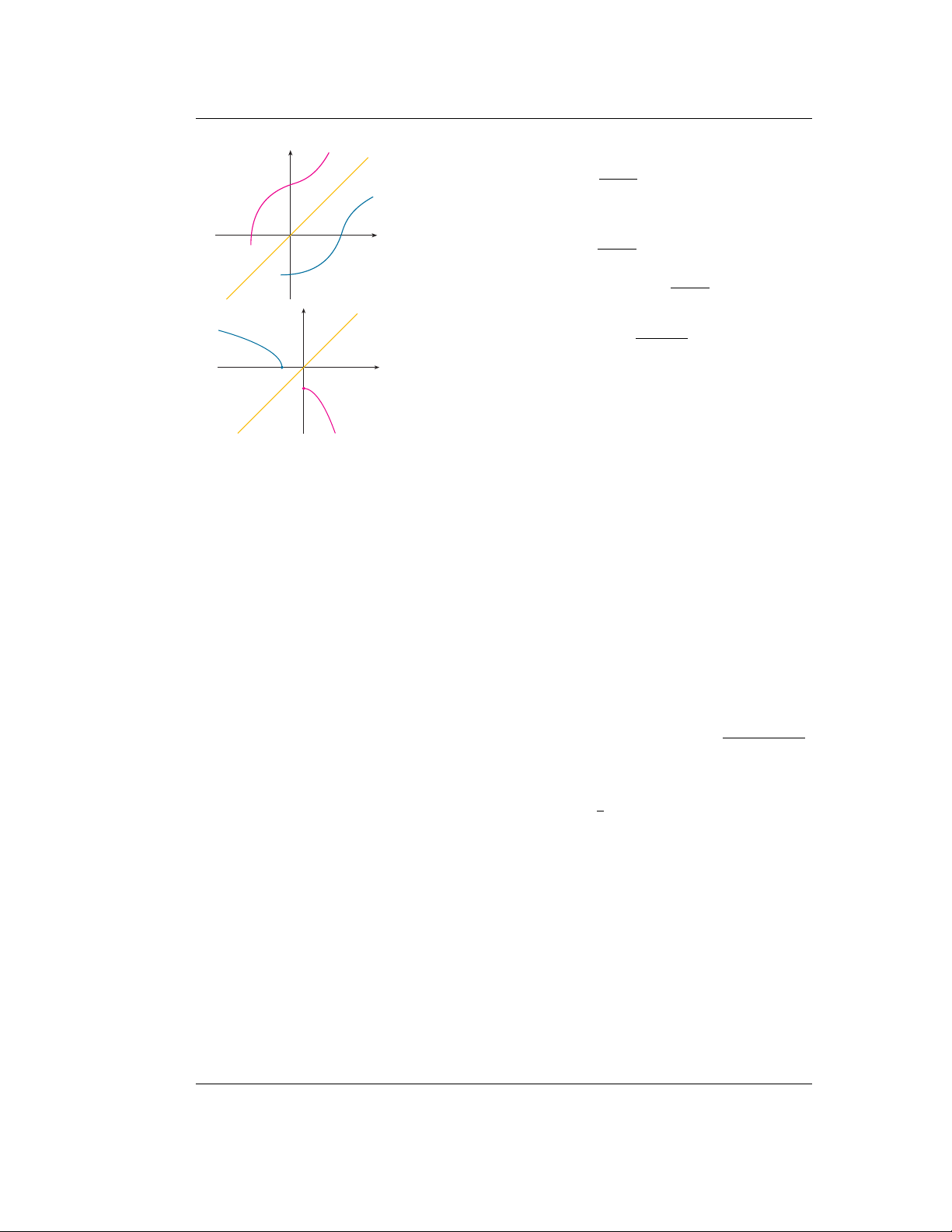
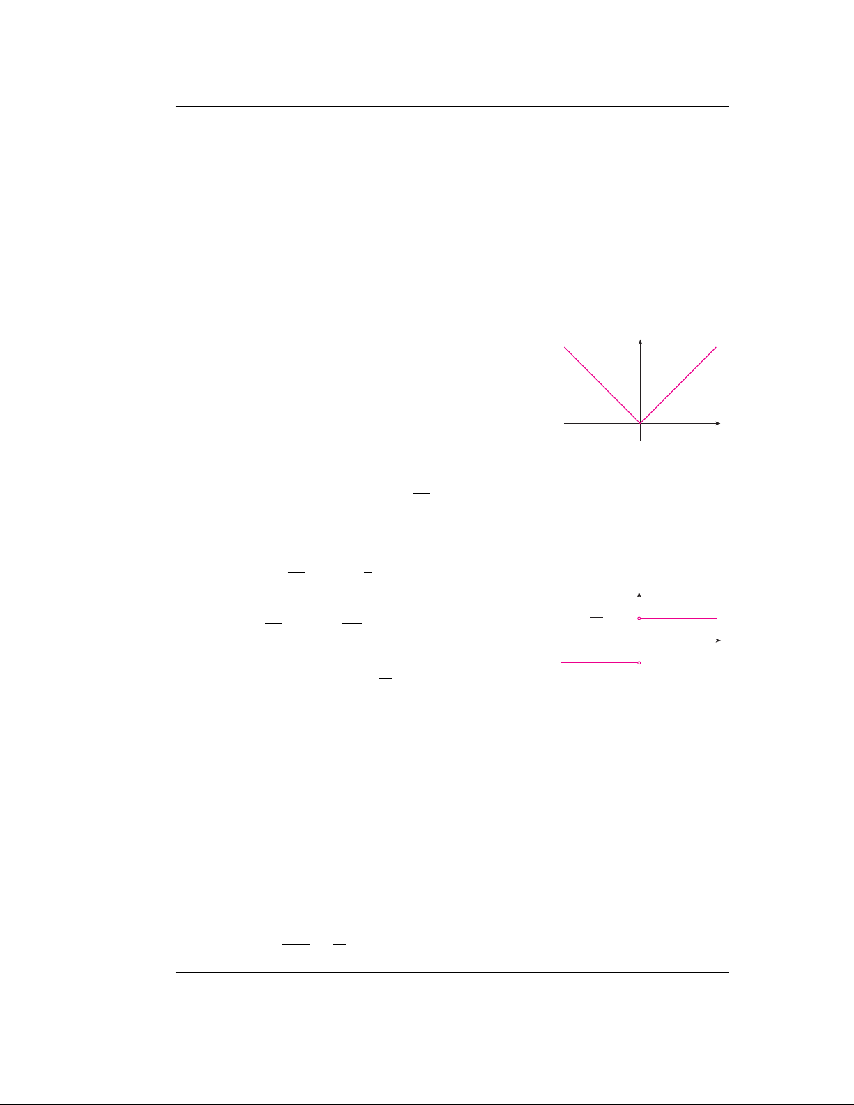
Hàm số chẵn, lẻ. Cho hàm số f xác định trên A, A là miền đối xứng qua gốc O. range y ⫽ ƒ(x) ƒ f (2)
• Hàm số f gọi là chẵn nếu f (x) = f (−x), ∀x ∈ A (Hình 1.1). Chẳng hạn hàm f (1)
f (x) = x2 là hàm số chẵn. 0 x 1 2 x 0 x domain
• Hàm số f gọi là lẻ nếu f (x) = −f (−x), ∀x ∈ A (Hình 1.1). Chẳng hạn hàm FIGURE 4 FIGURE 5 f (x) = x3 là hàm số lẻ. Hàm số đơn điệu.
• Hàm số f (x) được gọi là tăng trên A nếu ∀x1, x2 : x1 < x2 ⇒ f (x1) < f (x2).
• Hàm số f (x) được gọi là giảm trên A nếu ∀x1, x2 : x1 < x2 ⇒ f (x1) > f (x2).
• Hàm số f (x) được gọi là không tăng trên A nếu ∀x1, x2 : x1 < x2 ⇒ f (x1) ≥ f (x2). TS. NGUYỄN ĐỨC HẬU
http://nguyenduchau.wordpress.com 20 ■
CHAPTER 1 FUNCTIONS AND MODELS
We also see that the graph of f coincides with the x-axis for x ⬎ . Putting this 2
information together, we have the following three-piece formula for f : if 0 艋 x 艋 1
f 共x兲 苷 再x2 ⫺ x if 1 ⬍ x 艋 2 0 if x ⬎ 2
EXAMPLE 10 In Example C at the beginning of this section we considered the cost
C共w兲 of mailing a first-class letter with weight w. In effect, this is a piecewise C
defined function because, from the table of values, we have 0.34 if 0 ⬍ w 艋 1 1 0.56 if 1 ⬍ w 艋 2
C共w兲 苷 0.78 if 2 ⬍ w 艋 3 1.00 if 3 ⬍ w 艋 4 20 ■
CHAPTER 1 FUNCTIONS AND MODELS 0 1 2 3 4 5 w
The graph is shown in Figure 22. You can see why functions similar to this one are
We also see that the graph of f coincides with the x-axis for x ⬎ . Putting this 2
called step functions—they jump from one value to the next. Such functions will be
information together, we have the following three-piece formula for f : FIGURE 22 studied in Chapter 2. if 0 艋 x 艋 1
f 共x兲 苷 再x2 ⫺ x if 1 ⬍ x 艋 2 0 if x ⬎ 2 Symmetry
EXAMPLE 10 In Example C at the be y
ginning of this section we considered the cost
If a function f satisfies f 共⫺x兲 苷 f 共x兲 for every number x in its domain, then f is
C共w兲 of mailing a first-class letter with weight w. In effect, this is a piecewise
called an even function. For instance, the function f 共x兲 苷 x2 is even because C
defined function because, from the table of values, we have f (_x) ƒ 0.34 if 0 ⬍ w 艋 1
f 共⫺x兲 苷 共⫺x兲2 苷 x2 苷 f 共x兲 1 _x 0 x x 0.56 if 1 ⬍ w 艋 2
C共w兲 苷 0.78 if 2 ⬍ w 艋 3
The geometric significance of an even function is that its graph is symmetric with 1.00 if 3 ⬍ w 艋 4
respect to the y-axis (see Figure 23). This means that if we have plotted the graph of
f for x 艌 0, we obtain the entire graph simply by reflecting about the -axis. y 0 1 2 3 4 5 w
The graph is shown in Figure 22. You can see why functions similar to this one are
If f satisfies f 共⫺x兲 苷 ⫺f 共x兲 for every number x in its domain, then f is called an
called step functions—they jump from one value to the next. Such functions will be FIGURE 23
odd function. For example, the function f 共x兲 苷 x3 is odd because FIGURE 22 studied in Chapter 2. An even function
1.1. Hàm số một biến số 5
SECTION 1.1 FOUR WAYS TO REPRESENT A FUNCTION ◆ 21
f 共⫺x兲 苷 共⫺x兲3 苷 ⫺x3 苷 ⫺f 共x兲 Symmetry (c) y
h共⫺x兲 苷 2共⫺x兲 ⫺ 共⫺x兲2 苷 ⫺2x ⫺yx2
If a function f satisfies f 共⫺x兲 苷 f 共x兲 for every number x in its domain, then f is
The graph of an odd function is symmetric about the origin (see Figure 24). If we
Since h共⫺x兲 苷 h共x兲 and h共⫺x兲 苷 ⫺h共x , 兲 wcalled an ev e conclude that en h function is neither ev . For instance, en nor
the function f 共x already ha兲v苷 e x2 is even because
the graph of f for x 艌 0, we can obtain the entire graph by rotating odd. f (_x) ƒ
through 180⬚ about the origin. f
The graphs of the functions in Example 11 are sho 共
wn in Figure 25. Notice that the⫺x兲 苷 共⫺x兲2 苷 x 2 苷 f 共x兲 _x ƒ _x 0 graph of h 0 x x
is symmetric neither about the y-axis nor about the origin. x x
The geometric significance of an even function is that its graph is symmetric with y y y
EXAMPLE 11 Determine whether each of the following functions is even, odd, or 1
respect to the y-axis (see Figure 23). This means that if we have plotted the graph of 1 f g 1 h neither even nor odd.
f for x 艌 0, we obtain the entire graph simply by reflecting about the -axis. y (a) (b)
(c) h共x兲 苷 2x ⫺ x2
t共x兲 苷 1 ⫺ x 4
f 共x兲 苷 x5 ⫹ x
If 1 f satisfies f 共⫺x兲 苷 ⫺f 共x兲 for every number x in its domain, then f is called an x x x FIGURE 23 _1 1
odd function. For example, 1 the function f
Hình 1.1: Đồ thị hàm số chẵn (phải) và hàm số lẻ (trái).
共x兲 苷 x3 is odd because SOLUTION An even function _1 FIGURE 24
f 共⫺x兲 苷 共⫺x兲3 苷 ⫺
(a) x3 苷 ⫺f 共x兲
f 共⫺x兲 苷 共⫺x兲5 ⫹ 共⫺x兲 苷 共⫺1兲5x5 ⫹ 共⫺x兲 • Hàm số f FIGURE 25 (x) được (a) gọi là không An odd function giảm ( b) trên A nếu ∀x (c) y
1, x2 : x1 < x2 ⇒ f (x1) ≤
The graph of an odd function is symmetric about the origin (see Figure 24). If we
苷 ⫺x5 ⫺ x 苷 ⫺共x5 ⫹ x兲 f (x2).
already have the graph of f for x 艌 0, we can obtain the entire graph by rotating
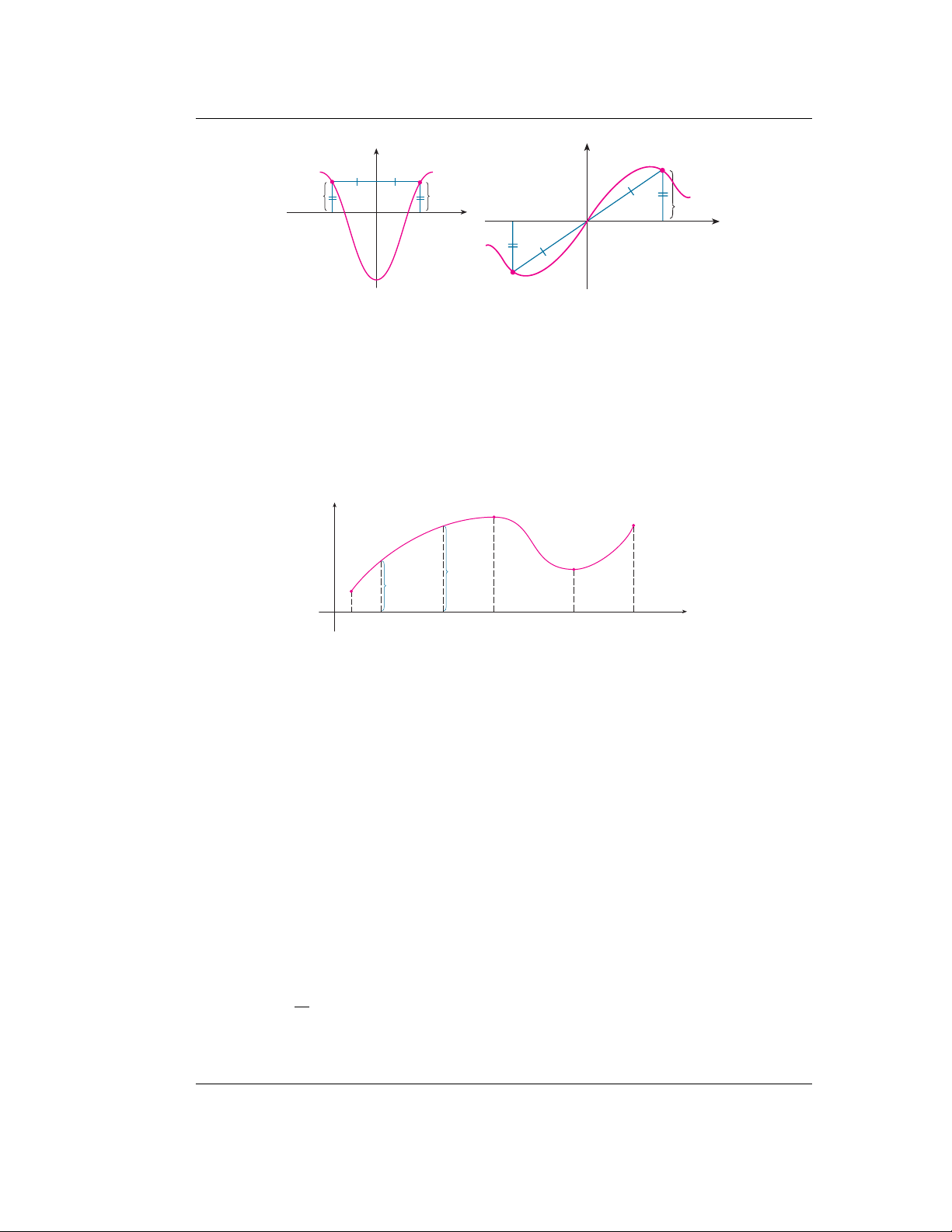
Increasing and Decreasing Functions
苷 ⫺f 共x兲
through 180⬚ about the origin. • Hàm số _x không tăng hay k ƒ
hông giảm trên A được gọi là hàm đơn điệu trên A. 0
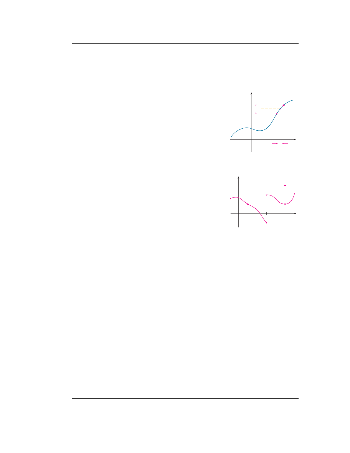
The graph shown in Figure 26 rises from A to ,
B falls from B to C, and rises again from C to D. x The function f x
is said to be increasing on the interval 关a, b , 兴 decreasing
Therefore, f is an odd function.
EXAMPLE 11 Determine whether each of the following functions is even, odd, or Trên hình 1.2, hàm on 关b, số c , 兴 tăng từ A lên
and increasing again on 关cB , d 兴 và giảm . Notice that if từ x1 B and x2 xuống are any tw C và lại o numbers tăng từ C lên
between a and b with x1 ⬍ x ,
2 then f 共x1 兲 neither e ⬍ f 共x2 . 兲 We ven nor odd.
use this as the defining prop-
D. Hàm f tăng trên các đoạn [a, b
erty of an increasing function. ], [c, d] và giảm trên đoạn [b, c]. t共⫺ (a) (b) (b)
(c) h共x兲 苷 2x ⫺ x2 x兲 苷 1 ⫺ 共⫺x兲4 苷 1 ⫺ x 4 苷 t共x兲
t共x兲 苷 1 ⫺ x 4
f 共x兲 苷 x5 ⫹ x y B SOLUTION D So is t even. FIGURE 24 y=ƒ (a)
f 共⫺x兲 苷 共⫺x兲5 ⫹ 共⫺x兲 苷 共⫺1兲5x5 ⫹ 共⫺x兲 An odd function
苷 ⫺x5 ⫺ x 苷 ⫺共x5 ⫹ x兲 C f(x™)
苷 ⫺f 共x兲 f(x ¡) A
Therefore, f is an odd function. 0 a x ¡ x™ b c d x FIGURE 26 (b)
t共⫺x兲 苷 1 ⫺ 共⫺x兲4 苷 1 ⫺ x 4 苷 t共x兲
Hình 1.2: Hàm số đơn điệu
A function f is called increasing So is t on an interval I e if ven.
f 共x1兲 ⬍ f 共x2兲
whenever x1 ⬍ x2 in I
Hàm bị chặn. Cho hàm số f (x) xác định trên A. y
It is called decreasing on if I y=≈
• Hàm f (x) được gọi là f共
bịxchặn trên nếu tồn tại M sao cho f (x) ≤ M , ∀x ∈ A.
1 兲 ⬎ f 共x2 兲
whenever x1 ⬍ x2 in I
• Hàm f (x) được gọi là bị chặn dưới nếu tồn tại M sao cho f (x) ≥ M , ∀x ∈ A.
In the definition of an increasing function it is important to realize that the inequal-
ity f 共x1兲 ⬍ f 共x2兲 must be satisfied for every pair of numbers x1 and x2 in I with 0 x x • 1 Hàm f (x) ⬍ x2.
được gọi là bị chặn (giới nội) nếu tồn tại M sao cho |f (x)| ≤ M ,
You can see from Figure 27 that the function f 共x兲 苷 x2 is decreasing on the inter- ∀ FIGURE 27 x ∈ A.
val 共⫺⬁, 0兴 and increasing on the interval 关0, ⬁ . 兲
Hàm số tuần hoàn. Cho hàm số f(x) xác định trên A. Nếu tồn tại số T dương sao
cho f (x + T ) = f (x), ∀x ∈ A thì f (x) được gọi là hàm số tuần hoàn. Số T nhỏ nhất
trong các số thoả mãn điều kiện trên gọi là chu kì của hàm số f (x).
Chú ý 1.1 (a) Các hàm số sin x, cos x là các hàm số tuần hoàn với chu kì là 2π.
(b) Các hàm số tan x, cot x là các hàm số tuần hoàn với chu kì là π.
(c) Nếu f (x) tuần hoàn với chu kì T thì hàm f (ax) cũng là hàm số tuần hoàn với chu kì là T . |a|
(d) Tổng hiệu các hàm số tuần hoàn với cùng một chu kì T cũng là hàm tuần
hoàn với chu kì T . Trường hợp các số hạng tuần hoàn nhưng khác chu kì, thì hàm TS. NGUYỄN ĐỨC HẬU
http://nguyenduchau.wordpress.com
1.1. Hàm số một biến số 6
tổng là hàm số tuần hoàn với chu kì là bội chung nhỏ nhất của các chu kì của các hàm số hạng. 44 ■
CHAPTER 1 FUNCTIONS AND MODELS
Ví dụ 1.1 (1) Hàm số y = a
The procedure is called cos(αx) composition + b sin(α because the ne x), α > w function is 0 là composedhàm số of the two tuần hoàn với chu kì là 2π . given functions and t f . α
In general, given any two functions and t f
, we start with a number x in the domain (2) Hàm số y of = t cos x + 1 and find its image cos(2 t共x兲 x) + 1 cos(3
. If this number t共x兲 x) là hàm
is in the domain of f số , tuần hoàn then we can cal- với chu kì là 2 3
culate the value of f 共t共x兲兲. The result is a new function h共x兲 苷 f 共t共x兲兲 obtained by 2π?
substituting t into f . It is called the composition (or composite) of and t f and is
denoted by f ⴰ t (“f circle t”).
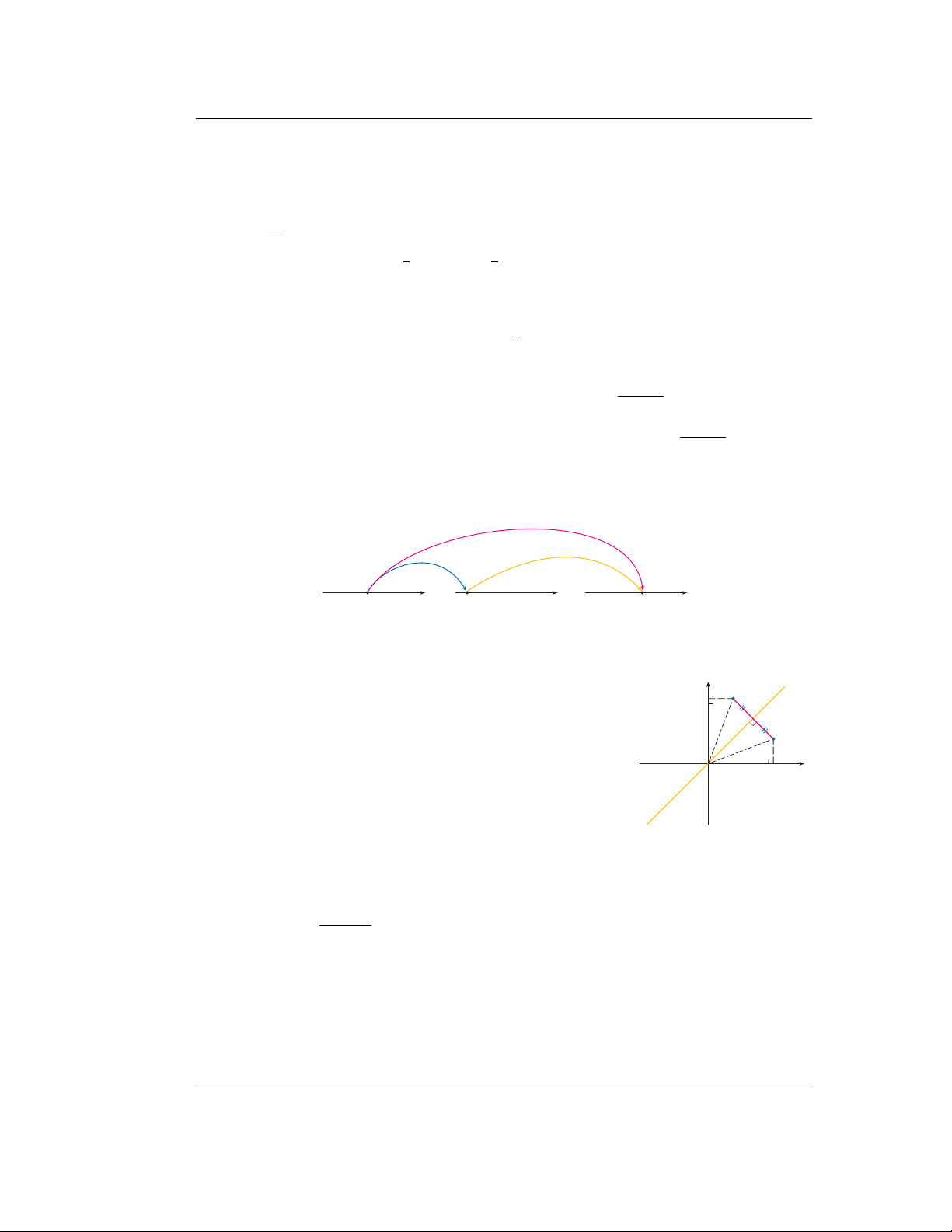
Hàm số hợp. Có nhiều cách khác nhau để tổ hợp hai hàm số thành một hàm số
Definition Given two functions and t f √
, the composite function f ⴰ t (also mới. Giả sử cho hai hàm called the số y = composition f of (u) and = t f u và
) is defined by u = g(x) = x2 + 1. Do y được biểu
diễn theo u và u lại được biểu diễn theo
共 f ⴰ t兲共xbiến 兲 苷 f 共t x
共x兲兲 nên ta có thể biểu diễn y theo x p y = f (u The domain of f)ⴰ = t f (g(x)) = is the set of all f (x2 + 1) = in the domain of t x x2 such that + t共x 1 兲 is in the
domain of f . In other words, 共 f ⴰ t兲共x兲 is defined whenever both t共x兲 and f 共t共x兲兲 are
defined. The best way to picture f ⴰ t √
is by a machine diagram (Figure 13) or an arrow
Quá trình trên tạo ra một diagram (Figure hàm 14).
số mới y = h(x) = f (g(x)) = x2 + 1 gọi là hàm hợp của f và g FIGURE 13
được kí hiệu bởi f ◦ g đọc là ’f o tròn g’.
The f • g machine is composed of x g g(x) f f{ ©} the g machine (first) and then (input) (output) the f machine. f • g f g FIGURE 14 Arrow diagram for f • g x © f{ ©} 68 ■
CHAPTER 1 FUNCTIONS AND MODELS
EXAMPLE 7 If f 共x兲 苷 x2 and t共x兲 苷 x ⫺ 3, find the composite functions f ⴰ t Hình 1.3: Hàm hợp
f ⫺1共b兲 苷 a 共a, b兲 f 共 and . if , the point
is on the graph of if and only if the point b, a兲 is on t ⴰ f
the graph of f ⫺ . But we get the point 1
共b, a兲 from 共a, b兲 by reflecting about the line SOLUTION We have
Hàm ngược. Cho hàm số f (x) là một song ánh (1 − 1) y 苷 x. (See Figure 8.) 共 f ⴰ y y
t兲共x兲 苷 f 共 t共x兲兲 苷 f 共x ⫺ 3兲 苷 共x ⫺ 3兲2 từ A lên B = f (A) ⊂ (b, a)
R (1 − 1 nghĩa là f (x1) 6= f (x2),
共t ⴰ f 兲共x兲 苷 t共 f 共x兲兲 苷 t共x2兲 苷 x2 ⫺ 3
∀x1 6= x2). Khi đó với mỗi y ∈ B ta có quy tắc kí hiệu là f –! f −1 xác định | đượNOTE
c duy nhất một x ∈ A sao cho f (x) = y.
● You can see from Example 7 that, in general, f ⴰ t 苷 t ⴰ f . Remember, the (a, b) notation means that the function t f ⴰ t
is applied first and then f is applied second.
Quy tắc f −1 đó được gọi là hàm ngược của hàm số f . Vậy 0 0
In Example 7, f ⴰ t is the function that first subtracts 3 and then squares; is t ⴰ f the x x y = f (x) ⇔ x function that = f −1(y) fir
. st squares and then subtracts 3.
Chú ý rằng nếu điểm (a, b) là một điểm thuộc đồ thị của y=x y=x f
EXAMPLE 8 If f 共x兲 苷 sx and t共x兲 苷 s2 ⫺ x, find each function and its domain. hàm f thì (b, a ( ) a) f th ⴰ t uộc đồ(b) t thị ⴰ fcủa f −1 (c) . (d) t ⴰ t f ⴰ f SOLUTION FIGURE 8 FIGURE 9 (a)
共 f ⴰ t兲共x兲 苷 f 共t共x兲兲 苷 f (s2 ⫺ x) 苷 ss2 ⫺ x 苷 s42 ⫺ x Therefore, as illustrated by Figure 9:
Ví dụ 1.2 Tìm hàm ngược của các hàm số
The domain of f ⴰ t is 兵x 苷 兵x y . ⱍ2 ⫺ x 艌 0其
ⱍx 艋 2其 苷 共⫺⬁, 2兴 y=ƒ
The graph of f ⫺1 is obtained by reflecting the graph of f about the line y 苷 x. (a) f (x) = x3 + 2 y=x √ (b) f (x) = −1 − x 0
EXAMPLE 5 Sketch the graphs of f 共x兲 苷 s⫺1 ⫺ x and its inverse function using the (_1, 0) x same coordinate axes. (0, _1) Giải.
SOLUTION First we sketch the curve y 苷 s⫺1 ⫺ x (the top half of the parabola
y 2 苷 ⫺1 ⫺ x, or x 苷 ⫺y2 ⫺ 1) and then we reflect about the line y 苷 x to get the y=f –!(x)
graph of f ⫺ . (See Figure 10.) 1
As a check on our graph, notice that the expression for f ⫺1 is
. So the graph of f ⫺1
f ⫺1共x兲 苷 ⫺x2 ⫺ 1, x 艌 0 is the right half of the FIGURE 10
parabola y 苷 ⫺x2 ⫺ 1 and this seems reasonable from Figure 10. Logarithmic Functions If a TS. NGUYỄN ĐỨC HẬU ⬎ 0 and
, the exponential function f 共x兲 苷 ax a 苷 1 is either increasing or
decreasing and so it is one-to-one by the Horizontal Line Test. It therefore has an
http://nguyenduchau.wordpress.com
inverse function f ⫺ , 1
which is called the logarithmic function with base a and is
denoted by log . If we use the formulation of an inverse function given by (3), a &?
f ⫺1共x兲 苷 y
f 共y兲 苷 x then we have &? 6 log x 苷 y a y a 苷 x Thus, if x ⬎ ,
0 then log x is the exponent to which the base a must be raised to give a
x. For example, log 0.001 苷 ⫺3 because 10⫺3 10 苷 . 0.001
The cancellation equations (4), when applied to f 共x兲 苷 ax and f ⫺1共x兲 苷 log x, a become 7
loga共ax兲 苷 x for every x 僆 ⺢
aloga x 苷 x for every x ⬎ 0 68 ■
CHAPTER 1 FUNCTIONS AND MODELS 68 ■
CHAPTER 1 FUNCTIONS AND MODELS
if f ⫺1共b兲 苷 a, the point 共a, b兲 is on the graph of f if and only if the point 共b, a兲 is on
the graph of f ⫺ . But we get the point 1
共b, a兲 from 共a, b兲 by reflecting about the line
y 苷 x. (See Figure 8.)
if f ⫺1共b兲 苷 a, the point 共a, b兲 1.1. Hàm is on the graph of f số một biến số
if and only if the point 共b, a兲 is on y y 7
the graph of f ⫺ . But we get the point 1
共b, a兲 from 共a, b兲 by reflecting about the line (b, a)
y 苷 x. (See Figure 8.)
(a) Giải phương trình y = x3 +f–2 ! theo biến x ta được y y (b, a) x3 = y − 2 hay (a, b) 0 0 f –! x = 3 py − 2 x x (a, b) Cuối cùng y=x
đổi chỗ của x với y ta y=x được f 0 0 x x √ y = 3 x − 2 y=x y=x f FIGURE 8 FIGURE 9
Therefore, as illustrated by Figure 9: √
Vậy hàm ngược cần tìm là f −1(x) = 3 x − 2. y FIGURE 8 FIGURE 9 y=ƒ
The graph of f ⫺1 is obtained by reflecting the graph of f about the line y 苷 x. y=x √
Therefore, as illustrated by Figure 9:
(b) Như hình vẽ đường cong y =
−1 − x là một nửa trên 0
EXAMPLE 5 Sketch the graphs of f 共x兲 苷 s⫺1 ⫺ x and its inverse function using the y
của parabol y2 = −1 − x hay x = −y2 − 1. Lấy đối xứng (_1, 0) x same coordinate axes. y=ƒ
The graph of f ⫺1 is obtained by reflecting the graph of f about the line (0, _1) y 苷 x. y=x
qua đường y = x ta được đồ thị của hàm f −1. Nó được
SOLUTION First we sketch the curve y 苷 s⫺1 ⫺ x (the top half of the parabola y 2 苷 biểu ⫺1 ⫺ x diễn , or b x ởi 苷 ⫺ f y − 2 1 ⫺
(x1) and then we reflect about the line ) = −x2 − 1, x ≥ 0. y V 苷 ậy x to get the đồ thị của y=f –!(x) 0
EXAMPLE 5 Sketch the graphs of f 共x兲 苷 s⫺1 ⫺ x and its inverse function using the
graph of f ⫺ . (See Figure 10.) 1
As a check on our graph, notice that the expression
f −1 là một nửa bên trái của parabol y = −x2 − 1. (_1, 0) x same coordinate axes. for f ⫺1 is
. So the graph of f ⫺1
f ⫺1共x兲 苷 ⫺x2 ⫺ 1, x 艌 0 is the right half of the (0, _1) FIGURE 10
Các hàm số sơ cấp cơ parabola y bản. 苷 ⫺x2 Các ⫺ 1
hàm and this seems reasonable from Figure 10.
số sau được gọi là hàm số sơ cấp cơ bản
SOLUTION First we sketch the curve y 苷 s⫺1 ⫺ x (the top half of the parabola
y 2 苷 ⫺1 ⫺ x, or x 苷 ⫺y2 ⫺ 1) and then we reflect about the line y 苷 x to get the y=f –!(x)
graph of f ⫺ . (See Figure 10.) 1 As a check on our graph, 1. Hàm notice that the e luỹ thừa x xpression α Logarithmic Functions . for f ⫺1 is
. So the graph of f ⫺1
f ⫺1共x兲 苷 ⫺x2 ⫺ 1, x 艌 0 is the right half of the If a ⬎ 0 and
, the exponential function f 共x兲 苷 ax a 苷 1 is either increasing or FIGURE 10
parabola y 苷 ⫺x2 ⫺ 1 and this seems reasonable from Figure 10.
decreasing and so it is one-to-one by the Horizontal Line Test. It therefore has an 2. Hàm mũ ax.
inverse function f ⫺ , 1
which is called the logarithmic function with base a and is Logarithmic Functions
denoted by log . If we use the formulation of an inverse function given by (3), a 3. Hàm số logarit loga x. &?
f ⫺1共x兲 苷 y
f 共y兲 苷 x If a ⬎ 0 and
, the exponential function f 共x兲 苷 ax a 苷 1 is either increasing or then we have
decreasing and so it is one-to-one by the Horizontal Line 4. Các T hàm est. It therefore has an
số lượng giác sin x, cos x, tan x, cot x.
inverse function f ⫺ , 1
which is called the logarithmic function with base a and is &? 6 log x 苷 y a y a 苷 x
denoted by log . If we use the formulation of an inverse function given by (3), a
5. Các hàm lượng giác ngược arcsin x, arccos x, arctan x, arccotx. &?
f ⫺1共x兲 苷 y
f 共y兲 苷 x Thus, if x ⬎ ,
0 then log x is the exponent to which the base a must be raised to give a then we have
Hàm sơ cấp. Hàm sơ cấ x p . For e là xample, các log hàm 0.001 được 苷 ⫺3 tạo because 10⫺3
thành bởi một số hữu hạn các phép 10 苷 . 0.001
The cancellation equations (4), when applied to f 共x兲 苷 ax and f ⫺1共x兲 苷 log x, a
tính đại số và phép hợp đối với các hàm số sơ cấp cơ bản. &? 6 log x 苷 y a y become a 苷 x ex + tan 6x 7 log4
Thus, if x ⬎ 0, then log x is the exponent to which the base Ví dụ 1.3 a (a) must be raised to gi Các hàm số y ve a
= cos 5x, y = x 共ax兲 + 苷 x for every x tan 3x − ln(僆 x ⺢ + 2), y = , a log
x. For example, log 0.001 苷 ⫺3 because 10⫺3
aloga x 苷 x for every x ⬎ 0 3 x − 3 10 苷 . 0.001
The cancellation equations (4), when applied to là các f 共 hàmx兲 苷 số ax sơand c f ⫺1
ấp. 共x兲 苷 log x, a become 0 khi x < 0
(b) Các hàm số y = |x|, y = sgnx, y = không phải là 1 − e− x2 khi x ≥ 0 7
loga共ax兲 苷 x for every x 僆 ⺢ các hàm số sơ cấp.
aloga x 苷 x for every x ⬎ 0
Hàm ẩn. Cho biểu thức F (x, y) = 0, (x, y) ∈ X × Y . Nếu ứng với x ∈ X ta xác
định được y ∈ Y thì ta nói biểu thức F (x, y) = 0 xác định cho ta hàm ẩn y đối với x.
Ví dụ 1.4 (a) Biểu thức x2 + 2x − y = 0 xác định hàm ẩn (biểu diễn dưới dạng
tường minh y theo x là y = x2 + 2x).
(b) Biểu thức exy + y = 0 xác định hàm ẩn nhưng không thể biểu diễn dưới dạng tường minh y theo x.
(c) Biểu thức x2 + y2 + 1 = 0 không xác định hàm ẩn. TS. NGUYỄN ĐỨC HẬU
http://nguyenduchau.wordpress.com
SECTION 1.7 PARAMETRIC CURVES ◆ 75
(The maximum charge capacity is Q and t is measured in
(e) reflecting about the line y 0 苷 x seconds.)
(f) reflecting about the x-axis and then about the line y 苷 x
(a) Find the inverse of this function and explain its meaning.
(g) reflecting about the y-axis and then about the line y 苷 x
(b) How long does it take to recharge the capacitor to 90%
(h) shifting 3 units to the left and then reflecting about the of capacity if a 苷 2? line y 苷 x
59. Starting with the graph of y 苷 ln x, find the equation of the
60. (a) If we shift a curve to the left, what happens to its reflec- graph that results from
tion about the line y 苷 x? In view of this geometric (a) shifting 3 units upward
principle, find an expression for the inverse of t
(b) shifting 3 units to the left
共x兲 苷 f 共x ⫹ c ,兲 where f is a one-to-one function.
(c) reflecting about the x-axis
(b) Find an expression for the inverse of h共x兲 苷 f 共cx , 兲
(d) reflecting about the y-axis where . c 苷 0
1.1. Hàm số một biến số 8 1.7 Parametric Curves ● ● ● ● ● ● ● ● ● ● ● ● ● ● ● ●
Hàm số theo tham số. Cho x = f (t), y = g(t) là các y
Imagine that a particle moves along the curve C shown in Figure 1. It is impossible to
hàm số cùng xác định trên T . Khi đó với mỗi x = f (t0) sẽ C
describe C by an equation of the form y 苷 f 共x兲 because C fails the Vertical Line Test.
cho ta y = g(t0) tại t0 xác định cho ta một hàm số y theo (x, y)={ f(t), g(t)}
But the x- and y-coordinates of the particle are functions of time and so we can write
đối số x gọi là hàm cho theo tham số x = f (t), y = g(t).
x 苷 f 共t兲 and y 苷 t共t . Such a pair of equations is often a con 兲 venient way of describ-
Với mỗi giá trị t xác định một điểm (x, y) trên mặt phẳng
ing a curve and gives rise to the following definition.
xOy. Khi t thay đổi điểm (x, y) = (f (t), g(t)) chạy trên
Suppose that x and y are both given as functions of a third variable t (called a
một đường cong C gọi là đường cong tham số. 0 x
parameter) by the equations
x 苷 f 共t兲 y 苷 t共t兲 FIGURE 1
(called parametric equations). Each value of t determines a point
Ví dụ 1.5 (a) Hàm số y = f (x) xác định trên X có thể viết dưới dạng tham số
共x, y ,兲 which we
can plot in a coordinate plane. As t varies, the point 共x, y兲 苷 共 f 共t兲, t共t兲兲 varies and x = t, y = f (t), t ∈ X.
traces out a curve C, which we call a parametric curve. The parameter t does not nec- x2 y2 (b) Hàm ẩn +
= 1 có thể viết dưới dạng tham số
essarily represent time and, in fact, we could use a letter other than t for the parame- a2 b2
ter. But in many applications of parametric curves, t does denote time and therefore
we can interpret 共x, y兲 苷 共 f 共t兲, t共t兲兲 as the position of a particle at time t. x = a cos t , 0 ≤ t ≤ 2π y = b sin t
EXAMPLE 1 Sketch and identify the curve defined by the parametric equations
x 苷 t2 ⫺ 2t y 苷 t ⫹ 1 Các hàm số hyperbolic.
SOLUTION Each value of t gives a point on the curve, as shown in the table. For ex − e−x
instance, if t 苷 0, then x 苷 0, y 苷 1 and so the corresponding point is 共0, 1 . In 兲
1. Hàm sine hyperbolic sinh x = . Figure 2 we plot the points 2
共x, y兲 determined by several values of the parameter and
we join them to produce a curve. ex + e−x
2. Hàm cosine hyperbolic cosh x = . y 2 t=4 t x y t=3 sinh x
3. Hàm tang hyperbolic tanh x = . ⫺2 8 ⫺1 t=2 cosh x ⫺1 3 0 0 0 1 t=1 cosh x (0, 1)
4. Hàm cotang hyperbolic coth x = . 1 ⫺1 2 t=0 8 sinh x 2 0 3 0 x 3 3 4 t=_1 5. Các hệ thức t=_2 4 8 5 cosh2 x − sinh2 x = 1 FIGURE 2 1 1 1 − tanh2 x = , 1 − coth2 x = cosh2 x sinh2 x
sinh(x + y) = sinh x cosh y + sinh y cosh x
sinh(x − y) = sinh x cosh y − sinh y cosh x
cosh(x + y) = cosh x cosh y + sinh y sinh x
cosh(x − y) = cosh x cosh y − sinh y sinh x Các hàm số khác. 1 1 sec x = , csc x = cos x sin x TS. NGUYỄN ĐỨC HẬU
http://nguyenduchau.wordpress.com
1.2. Giới hạn của dãy số thực 9 1.2.
Giới hạn của dãy số thực
Định nghĩa 1.2 (Dãy số) Cho hàm số f : N → R, n 7→ f (n) = an. Dãy các số
thực a1, a2,... được gọi là dãy số, an gọi là số hạng tổng quát của dãy số. Kí hiệu dãy số là {an}. Dãy bị chặn.
1. Dãy {an} gọi là bị chặn trên nếu tồn tại M sao cho an ≤ M , ∀n ∈ N.
2. Dãy {an} gọi là bị chặn dưới nếu tồn tại M sao cho an ≥ M , ∀n ∈ N.
3. Dãy {an} gọi là bị chặn (giới nội) nếu nó vừa bị chặn trên vừa bị chặn dưới
hay là tồn tại M sao cho |an| ≤ M , ∀n ∈ N.
Dãy đơn điệu. Dãy {an} gọi là đơn điệu tăng (tương ứng đơn điệu giảm) nếu
a1 ≤ a2 ≤ ... ≤ an ≤ ... (tương ứng a1 ≥ a2 ≥ ... ≥ an ≥ ...). Nếu không xảy ra dấu
bằng thì ta nói dãy là tăng giảm thực sự.
Định nghĩa 1.3 (Giới hạn hữu hạn của dãy số) Cho dãy số {an}. Số thực a
được gọi là giới hạn của dãy số an khi n → +∞ nếu như ∀ε > 0 bất kì cho trước
thì ∃N0 sao cho |an − a| < ε, ∀n ≥ N0. Kí hiệu là lim an = a hoặc an → a khi n→+∞
n → +∞. Hay còn nói {an} là dãy hội tụ đến a, trong trường hợp trái lại {an} gọi là dãy phân kì. Viết gọn lại
lim an = a ⇔ ∀ε > 0, ∃N0 : ∀n ≥ N0 ⇒ |an − a| < ε. n→+∞ Chú ý 1.2 Nếu
lim an = 0 thì dãy {an} được gọi là dãy vô cùng bé. n→+∞
Định nghĩa 1.4 (Dãy dần đến vô cùng)
lim an = ∞ ⇔ ∀M > 0, ∃N0 : ∀n ≥ N0 ⇒ |an| > M n→+∞ Các tính chất.
1. Giới hạn của dãy số nếu có là duy nhất.
2. Nếu an → a, bn → b khi n → +∞ (a, b hữu hạn) thì an ±bn → a±b, anbn → ab, an → a, b 6= 0. bn b
3. Cho hai dãy hội tụ {an}, {bn}
• Nếu tồn tại N0 ∈ N : an = bn, ∀n ≥ N0 thì lim an = lim bn. n→+∞ n→+∞
• Nếu tồn tại N0 ∈ N : an ≥ bn, ∀n ≥ N0 thì lim an ≥ lim bn. n→+∞ n→+∞ TS. NGUYỄN ĐỨC HẬU
http://nguyenduchau.wordpress.com
1.3. Giới hạn của hàm số thực 10
• Nếu tồn tại N0 ∈ N : an ≤ bn, ∀n ≥ N0 thì lim an ≤ lim bn. n→+∞ n→+∞
4. Cho 3 dãy {an}, {bn}, {cn}. Nếu an ≤ bn ≤ cn, ∀n và lim an = lim cn = L n→+∞ n→+∞ thì
lim bn = L (Giới hạn kẹp). n→+∞
5. Tích của một dãy bị chặn với dãy vô cùng bé là một dãy vô cùng bé.
6. Các giới hạn cần nhớ: 1 lim = 0 n→+∞ n lim qn = 0 ⇔ |q| < 1 n→+∞
APPENDIX D PRECISE DEFINITIONS OF LIMITS ◆ A31 lim qn = ∞ ⇔ |q| > 1 n→+∞
f 共x兲 x3 5x 6 lie in successively smaller intervals centered at 2 if the distance
from x to 1 is less than 1 n
. It turns out that it is always possible to find such a number lim 1 + = e , no matter ho n→+∞ n
w small the interval is. In other words, for any positive number , no
matter how small, there exists a positive number such that
ở đó e = 2, 718281828459045... là số vô tỉ. whenever
ⱍ共x3 5x 6兲 2ⱍ ⱍx 1ⱍ
Định lý 1.1 (Giới hạn của dãy đơn This indicates that
điệu) Dãy {an} là dãy đơn điệu tăng và bị
chặn trên thì hội tụ. Dãy {an} là dãy đơn điệu giảm lim 共x3 và 5x bị 6兲 chặn
2 dưới thì hội tụ. Dãy x l 1
{an} là dãy đơn điệu và không bị chặn thì sẽ là một dãy vô cùng lớn.
and suggests a more precise way of defining the limit of a general function. 1.3.
Giới hạn của hàm số thực
1 Definition Let f be a function defined on some open interval that contains the number ,
a except possibly at a itself. Then we say that the limit of f 共x兲 as
Định nghĩa 1.5 Số L đượ x c g appr ọi là giới oaches is a ,
L hạn của hàm and we write
số f (x) khi x dần đến a nếu
với bất kì dãy {xn} mà xn → a khi n → +∞ thì f (xn) → L khi n → +∞. Khi đó
lim f 共x兲 L
ta kí hiệu là lim f (x) = L. x l a x→a
if for every number 0 there is a corresponding number 0 such that ▲ The condition 0 is just ⱍx aⱍ Định another way of nghĩa saying that x 1 .6 a.
Số L được gọi là giới hạn của hàm số whenever
ⱍ f共x兲 Lⱍ f (x 0 ) khi ⱍx xaⱍdần đến a nếu
với ∀ε > 0 cho trước tìm được δ > 0 sao cho khi 0 < |x − a| < δ thì |f (x) − L| < ε. Viết gọn lại
Definition 1 is illustrated in Figures 3– 5. If a number 0 is given, then we draw
the horizontal lines y L and y L and the graph of f . (See Figure 3.) If lim f (x) = L ⇔ lim ∀ x lε a > f 共x兲0, ∃ Lδ
, > 0 : 0 < |x − a| < then we can find a number δ ⇒ 0 |f (x) − L| < ε
such that if we restrict x to lie in x→a
the interval 共a , a 兲 and take x a, then the curve y f 共x兲 lies between the
lines y L and y L . (See Figure 4.) You can see that if such a has been
found, then any smaller will also work. y y y y=ƒ L+∑ y=L+∑ y=L+∑ y=L+∑ ƒ ∑ ∑ L is in L ∑ ∑ here y=L-∑ y=L-∑ y=L-∑ L-∑ 0 a x 0 x 0 a a x a-∂ a+∂ a-∂ a+∂ when x is in here (x≠ a) TS. NGUYỄN ĐỨC HẬU FIGURE 3 FIGURE 4 http://nguyFIGURE 5 enduchau.wordpress.com
It’s important to realize that the process illustrated in Figures 3 and 4 must work
for every positive number no matter how small it is chosen. Figure 5 shows that if a
smaller is chosen, then a smaller may be required.
1.3. Giới hạn của hàm số thực 11 1
Ví dụ 1.6 Chứng minh rằng lim x cos = 0 x→0 x
Giải. ∀ε > 0 bé tuỳ ý, ta có 1 1 x cos − 0 = |x| cos x x
Nhận xét rằng khi 0 < |x| < ε thì 1 |x| cos < ε x
Vậy ta chọn δ = ε. Theo định nghĩa 1.6 ta có 1 lim x cos = 0 x→0 x 1
Ví dụ 1.7 Chứng minh rằng lim cos không tồn tại. x→0 x
Giải. Chọn hai dãy {xn}, {x0 } n ở đó 1 1 xn = x0 (π/2) + 2nπ n = 2nπ
Nhận xét khi n → +∞ thì xn → 0, x0 → n 0.
Mặt khác f (xn) = 0, f (x0n) = 1 do đó khi n → +∞ thì f(xn) → 0, f(x0n) → 1. Theo định nghĩa 1.5 thì 1 lim cos x→0 x không tồn tại.
Chú ý 1.3 Định nghĩa 1.5 và định nghĩa 1.6 là tương đương nhau. Người ta đã
chứng minh được rằng nếu f (x) là hàm số sơ cấp xác định tại a thì lim f (x) = f (a) x→a
Định nghĩa 1.7 Định nghĩa giới hạn của hàm số khi x → ∞.
lim f (x) = L ⇔ ∀ε > 0, ∃N > 0 : |x| > N ⇒ |f (x) − L| < ε x→∞ TS. NGUYỄN ĐỨC HẬU
http://nguyenduchau.wordpress.com
APPENDIX D PRECISE DEFINITIONS OF LIMITS ◆ A33 y
Therefore, by the definition of a limit, y=4x-5 7+∑ lim 共4x 5兲 7 7 x l3 7-∑
This example is illustrated by Figure 7.
Note that in the solution of Example 2 there were two stages—guessing and prov-
ing. We made a preliminary analysis that enabled us to guess a value for . But then
in the second stage we had to go back and prove in a careful, logical fashion that we
had made a correct guess. This procedure is typical of much of mathematics. Some- 0 x 3
times it is necessary to first make an intelligent guess about the answer to a problem
and then prove that the guess is correct. 3-∂ 3+∂
It’s not always easy to prove that limit statements are true using the , definition. FIGURE 7
For a more complicated function such as f 共x兲 共6x2 8x 9兲兾共2x2 1 , 兲 a proof
would require a great deal of ingenuity. Fortunately, this is not necessary because the
Limit Laws stated in Section 2.3 can be proved using Definition 1, and then the lim-
its of complicated functions can be found rigorously from the Limit Laws without
resorting to the definition directly. Limits at Infinity
Infinite limits and limits at infinity can also be defined in a precise way. The follow-
ing is a precise version of Definition 4 in Section 2.5.
2 Definition Let f be a function defined on some interval 共a, . 兲 Then
lim f 共x兲 L x l
means that for every 0 there is a corresponding number N such that whenever x N
ⱍ f共x兲 Lⱍ
In words, this says that the values of f 共x兲 can be made arbitrarily close to L
(within a distance , where is any positive number) by taking x sufficiently large
(larger than N, where N depends on ). Graphically it says that by choosing x large
enough (larger than some number N ) we can make the graph of f lie between the 106 ■
CHAPTER 2 LIMITS AND DERIVATIVES
given horizontal lines y L and y L as in Figure 8. This must be true no
matter how small we choose . If a smaller v
alue of is chosen, then a larger value of N may be required. y 1.3. Giới hạn EXAMPLE 6của hàm The Hea số thực
viside function H is defined by 12 y 1 if t y=ƒ 0 y=L +∑
H共t兲 苷 再0 ∑ 1 if t 0 ƒ is L 0 t ∑ in here y=L -∑
[This function is named after the electrical engineer Oliver Heaviside (1850–1925) FIGURE 8 0
and can be used to describe an electric current that is switched on at time t 苷 x .] Its 0 N FIGURE 8 graph is shown in Figure 8. lim ƒ=L when x is in here
As t approaches 0 from the left, H共t兲 approaches 0. As t approaches 0 from the x `
right, H共t兲 approaches 1. 1
There is no single number that H共t兲 approaches as t
Ví dụ 1.8 Chứng minh rằng lim = 0. approaches 0. Therefore, lim 共 x t →∞ l 0 H x t兲 does not exist.
Giải. ∀ε > 0 bé tuỳ ý. Ta có One-Sided Limits 1 1 1
We noticed in Example 6 that H共t兲 approaches 0 as t approaches 0 from the left and − 0 = < ε ⇔ |x| >
H共t兲 approaches 1 as t x |x|
approaches 0 from the right. We ε indicate this situation sym- bolically by writing
Chọn N = 1 theo định nghĩa 1.7 ta có ε
lim H共t兲 苷 0 and
lim H共t兲 苷 1 t l 0 t l 0 1 The symbol “t l 0 ” lim = 0
indicates that we consider only values of t that are less than 0. x→∞ x
Likewise, “t l 0” indicates that we consider only values of t that are greater than 0. Chú ý 1. 24 Tương Definition tự W ta e có write thể định nghĩa:
lim f 共x兲 苷 L
lim f (x) = ∞ ⇔ ∀M > 0 x , l ∃
aε > 0 : |x − a| < ε ⇒ |f (x)| > M x→a
and say the left-hand limit of f 共x兲 as x approaches a [or the limit of f 共x兲 as
lim f (x) = ∞ ⇔ ∀M > 0, ∃N > 0 : |x| > N ⇒ |f (x)| > M x x→∞
approaches a from the left] is equal to L if we can make the values of f 共x兲
as close to L as we like by taking x to be sufficiently close to a and x less than a.
Định nghĩa 1.8 (Giới hạn một phía) Giới hạn phải
Notice that Definition 2 differs from Definition 1 only in that we require x to be lim f (x) = lim f (x) = lim f (x) = f (a + 0) less than a x→a
. Similarly, if we require that x be greater than a, we get “the right-hand x→a+ x→a+0 x>a
limit of f 共x兲 as x approaches a is equal to L” and we write Giới hạn trái
lim f 共x兲 苷 L x l a lim f (x) = lim f (x) = lim f (x) = f (a − 0) x→a
Thus, the symbol “x l a” x→a− x→a−0
means that we consider only x a. These definitions are xillustrated in Figure 9. y y L ƒ L ƒ 0 x a x 0 a x x FIGURE 9 (a) lim ƒ=L (b) lim ƒ=L x a_ x a+ TS. NGUYỄN ĐỨC HẬU
http://nguyenduchau.wordpress.com
SECTION 2.3 CALCULATING LIMITS USING THE LIMIT LAWS ◆ 115
Some limits are best calculated by first finding the left- and right-hand limits. The
following theorem is a reminder of what we discovered in Section 2.2. It says that a
two-sided limit exists if and only if both of the one-sided limits exist and are equal.
SECTION 2.3 CALCULATING LIMITS USING THE LIMIT LAWS ◆ 115 1 Theorem
lim f 共x兲 苷 L if and only if
lim f 共x兲 苷 L 苷 lim f 共x兲 x l a x l a
Some limits are best calculated by first finding the left- and right-hand limits. x l a The
1.3. Giới hạn của hàm số thực 13
following theorem is a reminder of what we discovered in Section 2.2. It says that a
two-sided limit exists if and only if both of the one-sided limits exist and are equal.
When computing one-sided limits we use the fact that the Limit Laws also hold for Định lý 1.2 one-sided limits.
lim f (x) = L ⇔ lim f (x) = L = lim f (x) 1 Theorem
lim f 共x兲 苷 L if and only if
lim f 共x兲 苷 L 苷 lim f 共x兲 x l a x l a x l a x→a x→a− EXAMPLE 7 Sho x→ w that a+ lim ⱍxⱍ 苷 0 . x l 0 SOLUTION Recall that
When computing one-sided limits we use the fact that the Limit Laws also hold for one-sided limits.
Ví dụ 1.9 Chứng minh rằng lim |x| = 0. ⱍ if x 0 x ⱍ 苷 再x x→0 x if x 0
EXAMPLE 7 Show that lim
▲ The result of Example 7 looks ⱍxⱍ 苷 0 . x l 0 plausible from Figure 3. Since for x 0, we have ⱍxⱍ 苷 x Giải. Ta có SOLUTION Recall that y
lim ⱍxⱍ 苷 lim x 苷 0 if x 0 x khi x ≥ 0 x l 0 x l 0 y=| x | ⱍxⱍ 苷 再x |x| = x if x 0 −x khi x < 0 For we x 0 have ▲ The result of Example and so 7 looks ⱍxⱍ 苷 x plausible from Figure 3. Since for x 0, we have ⱍxⱍ 苷 x
lim ⱍxⱍ 苷 lim 共x兲 苷 0 Do đó y x l 0 x l 0
lim ⱍxⱍ 苷 lim x 苷 0 x l 0 x l 0 lim |x 0 | = lim x = x 0 y=| x | Therefore, by Theorem 1, x→0+ x→0+ For we x 0 have and so lim ⱍxⱍ 苷 0 ⱍxⱍ 苷 x x l 0 lim FIGURE 3 |x| = lim (−x) = 0
lim ⱍxⱍ 苷 lim 共x兲 苷 0 x→0− x→0− x l 0 x l 0 ⱍxⱍ
EXAMPLE 8 Prove that lim does not exist.
Sử dụng định lý 1.2 ta nhận được lim |x| = 0. x l 0 0 x x Therefore, by Theorem 1, x→0 lim ⱍxⱍ 苷 0 x l 0 FIGURE 3 ⱍxⱍ x SOLUTION lim 苷 lim 苷 lim 1 苷 1 |x| x l 0 x x l 0 x x l 0 ⱍxⱍ
EXAMPLE 8 Prove that lim
Ví dụ 1.10 Chứng minh rằng lim không tồn tại. does not exist. x l 0 x x→0 x ⱍxⱍ x lim 苷 lim 苷 lim 共1兲 苷 1 x l 0 x x l 0 x x l 0 ⱍxⱍ x SOLUTION lim Giải. Ta có 苷 lim 苷 lim 1 苷 1 x l 0 x x l 0 x x l 0
Since the right- and left-hand limits are different, it follows from Theorem 1 that |x| x lim
does not exist. The graph of the function f ⱍxⱍ兾x x l 0 共x兲 苷 is shown in ⱍxⱍ兾x lim = lim = lim 1 = 1 ⱍxⱍ x
Figure 4 and supports the limits that we found. lim 苷 lim 苷 lim 共1兲 苷 1 x→0+ x x→0+ x x→0+ x l 0 x x l 0 x x l 0 y | x |
Since the right- and left-hand limits are different, it follows from Theorem 1 that |x| −x y= lim = lim = lim (−1) = −1 1 x lim
does not exist. The graph of the function f x x ⱍxⱍ兾x x l 0 共x兲 苷 is shown in ⱍxⱍ兾x x→0− x→0− x→0−
Figure 4 and supports the limits that we found. 0 x y
Do các giới hạn trái và giới hạn phải khác nhau nên _1 | | x | x| y=
theo định lý 1.2 ta suy ra lim không tồn tại. 1 x x→0 xFIGURE 4 Các tính chất. 0 x
EXAMPLE 9 The greatest integer function is defined by 冀x冁 苷 the largest integer _1
▲ Other notations for 冀x冁 are 关x兴 and x.
that is less than or equal to x. (For instance, 冀4冁 苷 4, 冀4.8冁 苷 , 4 冀冁 苷 , 3 冀s2 冁 苷 , 1
1. lim C = C, ∀x0 là hữu hạn hay bằng ∞. FIGURE 4 x→x0 冀1冁 苷 1. 2 ) Show that lim
冀x冁 does not exist. x l3
EXAMPLE 9 The greatest integer function is defined by
2. Giới hạn của hàm số trong một quá trình nếu có là duy nhất.
冀x冁 苷 the largest integer
▲ Other notations for 冀x冁 are 关x兴 and x.
that is less than or equal to x. (For instance, 冀4冁 苷 4, 冀4.8冁 苷 , 4 冀冁 苷 , 3 冀s2 冁 苷 , 1
3. Cho lim f1(x) = L1, lim f2(x) = L2. Khi đó: 冀1冁 苷 1. 2 ) Show that lim
冀x冁 does not exist. x l3 x→x0 x→x0
• lim Cf1(x) = CL1, C là hằng số. x→x0
• lim [f1(x) + f2(x)] = L1 + L2 x→x0 • lim [f1(x)f2(x)] = L1L2 x→x0 • lim f1(x) = L1 , L2 6= 0 x→x f L2 0 2(x) TS. NGUYỄN ĐỨC HẬU
http://nguyenduchau.wordpress.com
1.3. Giới hạn của hàm số thực 14
Chú ý 1.5 Trong các tính chất trên L1, L2 là hữu hạn. Khi L1, L2 là vô hạn ta có
các dạng vô định. Khi gặp phải các dạng vô định thì phải khử đưa về trường hợp hữu
hạn sau đó mới áp dụng các tính chất trên. Các dạng vô định thường gặp ∞ − ∞, 0 × ∞, 0 , ∞ . 0 ∞
Bảng các giới hạn cơ bản. 1 1 1. lim = ∞, lim = 0 x→0 x x→∞ x +∞, a > 1 0, a > 1 2. lim ax = , lim ax = x→+∞ 0, 0 < a < 1 x→−∞ +∞, 0 < a < 1 +∞, a > 1 −∞, a > 1 3. lim loga x = , lim loga x = x→+∞ −∞, 0 < a < 1 x→0+ +∞, 0 < a < 1 π π 4. lim arctan x = , lim arctan x = − x→+∞ 2 x→−∞ 2 5. lim arccotx = 0, lim arccotx = π x→+∞ x→−∞ anxn + an−1xn−1 + ... + a0 6. lim
bằng an nếu m = n, bằng 0 nếu n < m và x→∞ b bm mxm + bm−1xm−1 + ... + b0 bằng ∞ nếu n > m. sin x sin x 7. lim = 1, lim = 0 x→0 x x→∞ x 1 x 1 8. lim 1 + = e, lim (1 + x) x = e x→∞ x x→0 log 1 ln(1 + x) 9. lim a(1 + x) = , lim = 1 x→0 x ln a x→0 x ax − 1 ex − 1 10. lim = ln a, lim = 1 x→0 x x→0 x √ (1 + x)α − 1 n 1 + x − 1 1 11. lim = α, lim = x→0 x x→0 x n
Ví dụ 1.11 Sử dụng bảng giới hạn cơ bản ta có sin 2x sin 2x 1. lim = 2 lim = 2 x→0 x x→0 2x 1 h 1 i2
2. lim (1 + 2x) x = lim (1 + 2x)2 1 2x = lim (1 + 2x) 2x = e2 x→0 x→0 x→0 ex − e−x ex − 1 e−x − 1 3. lim = lim + lim = 1 + 1 = 2 x→0 x x→0 x x→0 −x TS. NGUYỄN ĐỨC HẬU
http://nguyenduchau.wordpress.com
1.3. Giới hạn của hàm số thực 15 Các dạng vô định khác. lim [f (x)]g(x) x→a
1. lim f (x) = 0 và lim g(x) = 0 dạng 00 x→a x→a
2. lim f (x) = ∞ và lim g(x) = 0 dạng ∞0 x→a x→a
3. lim f (x) = 1 và lim g(x) = ±∞ dạng 1∞ x→a x→a
Thông thường ta sử dụng đẳng thức sau trong quá trình tính các giới hạn dạng trên
[f (x)]g(x) = exp[g(x) ln f (x)]
Ví dụ 1.12 Dùng công thức trên ta có thể tính được giới hạn dạng 1∞ sau 1 1 1 + tan x sin3 x tan x − sin x sin3 x lim = lim 1 + x→0 1 + sin x x→0 1 + sin x 1 tan x − sin x = lim exp ln 1 + x→0 sin3 x 1 + sin x 1 tan x − sin x tan x − sin x tan x − sin x = lim exp ln 1 + : x→0 sin3 x 1 + sin x 1 + sin x 1 + sin x Xét giới hạn 1 tan x − sin x 1 − cos x 1 lim = lim = x→0 sin3 x 1 + sin x x→0 sin2 x(1 + sin x) cos x 2 Từ đó suy ra 1 1 + tan x sin3 x √ lim = e x→0 1 + sin x
Định lý 1.3 Cho ba hàm số f (x), g(x), h(x) thoả mãn f (x) ≤ g(x) ≤ h(x), ∀x ∈
(a, b). Điểm x0 ∈ [a, b]. Khi đó nếu lim f (x) = lim h(x) = L thì lim g(x) = L. x→x0 x→x0 x→x0 1
Ví dụ 1.13 Chứng minh rằng lim x2 sin = 0. x→0 x TS. NGUYỄN ĐỨC HẬU
http://nguyenduchau.wordpress.com
1.3. Giới hạn của hàm số thực 16
SECTION 2.3 CALCULATING LIMITS USING THE LIMIT LAWS ◆ 117 Giải. Ta có đánh giá y y=≈ 1 −1 ≤ sin ≤ 1 1 y=≈ sin x x
Watch an animation of a similar limit. Resources / Module 2 0 x / Basics of Limits / Sound of a Limit that Exists do đó 1 −x2 ≤ x2 sin ≤ x2 y=_≈ FIGURE 7 x We know that lim x 2
Áp dụng định lý 1.3 ta nhận được lim x2 sin 1 = 0. 苷 0 and lim x2 苷 0 x l 0 x l 0 x→0 x
Taking f 共x兲 苷 x , 2
, and h共x兲 苷 x2
t共x兲 苷 x 2 sin共1兾x兲 in the Squeeze Theorem, we obtain
Vô cùng bé, vô cùng lớn. 1 lim x 2 sin 苷 0 x l0 x
Định nghĩa 1.9 (Vô cùng bé) Hàm f (x) gọi là vô cùng bé (VCB) khi x → x Exercises 0 ● ● ● ● ● ● ● ● ● ● ● ● ● ● ● ● ● ● ● ● ● ● ● ● ● ● 2.3
(x0 có thể hữu hạn hay vô hạn) nếu lim f (x) = 0. 1. Given that f 共x兲
(c) lim 关 f 共x兲t共x兲兴 (d) lim x x→x l 0 x l 1 t
0 lim f 共x兲 苷 3 lim t共x兲 苷 0
lim h共x兲 苷 8 共x兲 x l a x l a x l a
find the limits that exist. If the limit does not exist, explain
(e) lim x 3f 共x兲
(f) lim s3 f 共x兲 x l 2 x l 1 why. (a)
关 f 共x兲 h共x兲兴 (b) lim
关 f 共x兲兴2 lim
3–7 ■ Evaluate the limit and justify each step by indicating the x la x la appropriate Limit Law(s).
Ví dụ 1.14 (1) Hàm f (x) = xn là một VCB khi x → 0, ∀n ≥ 1. 1 (c) lim s 3 h共x兲 (d) lim 2x2 1 x l a
x l a f 共x兲
3. lim 共5x2 2x 3兲 4. lim x l 4
x l 2 x2 6x 4 t f 共x兲 共x兲
(2) 1 − cos x là một VCB khi x → 0. (e) lim (f) lim x l a x l a h共x兲 f 共x兲
5. lim 共t 1兲9共t2 1兲 6. lim su 4 3u 6 t l 2 u l 2 f 共x兲 2 f 共x兲 (g) lim (h) lim x l a t x l a 共x兲
h共x兲 f 共x兲
(3) 0 là VCB trong mọi quá trình. 7.
2. The graphs of f and t are given. Use them to evaluate each 冉 13x 冊3 lim x l 1 1 4x2 3x4 ■ ■ ■ ■ ■ ■ ■ ■ ■ ■ ■ ■ ■
limit, if it exists. If the limit does not exist, explain why. y y
8. (a) What is wrong with the following equation? y=ƒ y=© x 2 x 6 Tính chất. 1 1 苷 x 3 x 2 1 x 0 1 x
(b) In view of part (a), explain why the equation x 2 x 6 lim 苷 lim 共x 3兲
1. Nếu f (x) là VCB khi x → x x l 2
0 thì C f (x) là VCB khi x → x0 (C là hằng số). x 2 x l 2
(a) lim 关 f 共x兲 t共x兲兴 (b) lim
关 f 共x兲 t共x兲兴 x l2 x l1 is correct.
2. Tích, tổng của các VCB khi x → x0 là một vô cùng bé khi x → x0.
3. Tích của một VCB với một hàm bị chặn là một VCB trong cùng một quá trình.
Ví dụ 1.15 Hàm f (x) = x sin 1 là một VCB khi x → 0 vì trong quá trình đó x là x
một VCB còn sin 1 là hàm bị chặn. x
Quan hệ giữa VCB và hàm có giới hạn hữu hạn.
lim f (x) = L ⇔ f (x) − L là VCB khi x → x0 x→x0
⇒ f (x) = L + α(x), α(x) là VCB khi x → x0
So sánh các đại lượng VCB. Cho f (x) và g(x) là hai VCB trong cùng một quá trình.
1. Nếu lim f(x) = 0 thì ta nói f (x) là VCB cấp cao hơn g(x) hay g(x) là VCB g(x)
cấp thấp hơn f (x). Kí hiệu là f (x) = o(g(x)) (Nhận xét: Nếu g(x) là VCB cấp
thấp hơn f (x) thì lim g(x) = ∞). f (x)
2. Nếu lim f(x) = k (k 6= 0, k hữu hạn) thì ta nói f (x) và g(x) là hai VCB cùng g(x)
cấp. Kí hiệu là f (x) = O(g(x)).
Đặc biệt nếu k = 1 thì ta nói f (x) và g(x) là hai VCB tương đương. Kí hiệu là f (x) ∼ g(x). TS. NGUYỄN ĐỨC HẬU
http://nguyenduchau.wordpress.com
1.3. Giới hạn của hàm số thực 17
3. Nếu không tồn tại giới hạn lim f(x) thì ta nói f (x) và g(x) là hai VCB không g(x) so sánh được.
Ví dụ 1.16 Trong quá trình x → 0 thì x, x2, 1 − cos x, x2/2, x cos(1/x) là các VCB. Giải. 1 − cos x 2 sin2(x/2) 1. Vì lim = lim = 0 nên 1 − cos x = o(x). x→0 x x→0 x x 2. Vì lim = ∞ nên x2 = o(x). x→0 x2 1 − cos x 2 sin2(x/2) 1 3. Vì lim = lim = nên 1 − cos x = O(x2). x→0 x2 x→0 x2 2 1 − cos x 2 sin2(x/2) 4. Vì lim = lim = 1 nên 1 − cos x ∼ x2/2. x→0 x2/2 x→0 x2/2 x cos(1/x)
5. Vì không tồn tại giới hạn lim
nên x cos(1/x) và x là hai VCB không x→0 x so sánh được.
Hai quy tắc thay thế VCB tương đương và ngắt bỏ VCB cấp cao.
Quy tắc 1. Cho f1(x), g1(x), f2(x), g2(x) là các VCB trong cùng một quá trình
nào đó. Nếu f1(x) ∼ f2(x) và g1(x) ∼ g2(x) thì f1(x) f2(x) lim = lim g1(x) g2(x)
Ví dụ 1.17 Tính giới hạn ln(1 + 2x) lim x→0 sin 5x
Giải. Do ln(1 + 2x) ∼ 2x, sin 5x ∼ 5x (x → 0) nên ta có ln(1 + 2x) 2x 2 lim = lim = x→0 sin 5x x→0 5x 5
Chú ý 1.6 Cho f (x) và g(x) là hai VCB trong cùng một quá trình nào đó. Nếu
f (x) = o(g(x)) thì f (x) + g(x) ∼ g(x). TS. NGUYỄN ĐỨC HẬU
http://nguyenduchau.wordpress.com
1.3. Giới hạn của hàm số thực 18
Quy tắc 2. Cho f (x) = f1(x)+f2(x)+...+fn(x), g(x) = g1(x)+g2(x)+...+gm(x)
là tổng của các VCB trong cùng một quá trình nào đó. Nếu f1(x) là VCB cấp thấp
hơn so với các vô cùng bé fi(x), i = 2, ..., n và g1(x) là VCB cấp thấp hơn so với các
VCB gj(x), j = 2, ..., m. Khi đó f (x) f1(x) + f2(x) + ... + fn (x) f1(x) lim = lim = lim g(x) g1(x) + g2(x) + ... + gm(x) g1(x)
Ví dụ 1.18 Tính giới hạn x + 1 − cos x + tan3 x lim x→0 2x + sin2 x + 3x5
Giải. Do 1 − cos x = O(x), tan3 x = O(x) (x → 0) và sin2 x = O(2x), 3x5 = O(2x) (x → 0) nên ta có x + 1 − cos x + tan3 x x 1 lim = lim = x→0 2x + sin2 x + 3x5 x→0 2x 2 Chú ý 1.7
1. Số 0 là VCB cấp cao nhất trong mọi quá trình.
2. Nếu f1(x) ∼ g1(x), f2(x) ∼ g2(x) thì là các VCB tương đương trong cùng một
quá trình thì f1(x)f2(x) ∼ g1(x)g2(x).
3. Trong cùng một quá trình nào đó nếu f1(x) ∼ f2(x) thì f1(x) − f2(x) =
o(f1(x)). Có nghĩa là không thể thay thế tương đương trong từng hạng tử của
biểu thức hiệu của hai VCB tương đương. tan x − sin x Ví dụ 1.19 Tính lim x→0 x3 Giải. tan x − sin x sin x(1 − cos x) 1 sin x 2 sin2 x 1 lim = lim = lim 2 = x→0 x3 x→0 x3 cos x x→0 cos x x x2 2
Chú ý 1.8 Nếu thay thế tương đương tan x ∼ x và sin x ∼ x (x → 0) ta sẽ thu được
giới hạn trên bằng 0. Cách làm này dẫn đến kết quả sai.
Các vô cùng bé tương đương cần nhớ. Trong quá trình x → 0 thì ta có các VCB
tương đương sau: sin x ∼ x, arcsin x ∼ x, tan x ∼ x, arctan x ∼ x, 1 − cos x ∼ x2/2,
ln(1 + x) ∼ x, ex − 1 ∼ x, (1 + x)µ − 1 ∼ µx.
Định nghĩa 1.10 (Vô cùng lớn) Hàm f (x) gọi là vô cùng lớn (VCL) khi x → x0
(x0 có thể hữu hạn hay vô hạn) nếu lim f (x) = ∞. x→x0
Tương tự như trên giống như VCB ta cũng có thể so sánh các đại lượng VCL và hai
quy tắc thay thế VCL tương đương và ngắt bỏ VCL cấp thấp. TS. NGUYỄN ĐỨC HẬU
http://nguyenduchau.wordpress.com SECTION 2.4 CONTINUITY ◆ 119
41. Show by means of an example that lim
point of intersection of the two circles, and R is the point of
关 f 共x兲 t共x兲兴 x l a
may exist even though neither lim
f 共x兲 nor lim t
intersection of the line PQ and the x-axis. What happens to x l a 共x兲 x l a exists. R as shrinks, that is, as r l 0 C ? 2
42. Show by means of an example that lim
关 f 共x兲t共x兲兴 may x l a y exist even though neither lim
f 共x兲 nor lim t x l a 共x兲 x l a exists. P Q
43. Is there a number a such that C™
3x 2 ax a 3 lim x l 2 x 2 x 2 0 R x
exists? If so, find the value of a and the value of the limit. C¡
44. The figure shows a fixed circle C with equation 1
共x 1兲2 y2 苷 1 and a shrinking circle C with radius r 2
and center the origin. P is the point 共0, r , 兲 Q is the upper 2.4 Continuity ● ● ● ● ● ● ● ● ● ● ● ● ● ● ● ● ● ●
Explore continuous functions interactively.
We noticed in Section 2.3 that the limit of a function as x approaches a can often Resources / Module 2
be found simply by calculating the value of the function at . Functions with this a / Continuity
property are called continuous at a. We will see that the mathematical definition of / Start of Continuity
continuity corresponds closely with the meaning of the word continuity in everyday
language. (A continuous process is one that takes place gradually, without interrup- tion or abrupt change.)
1 Definition A function f is continuous at a number a if
lim f 共x兲 苷 f 共a兲 1.4. Hàm số liên tục 19 x la 1.4. Hàm số liên tục
If f is not continuous at a, we say f is discontinuous at a, or has f a discontinuity
at a. Notice that Definition l implicitly requires three things if f is continuous at a:
▲ As illustrated in Figure 1, if f is con-
1. f 共a兲 is defined (that is, a is in the domain of f )
Định nghĩa 1.11 Hàm f (x) được gọi là liên tục tại
tinuous, then the points 共x, f 共x兲兲 on the f 2. lim f
graph of approach the point 共a, f 共a兲兲 共x兲 exists điểm a nếu: x la
on the graph. So there is no gap in the 3. lim f curve.
共x兲 苷 f 共a兲 x la
• Hàm f (x) xác định tại điểm a và lân cận của điểm y y=ƒ
The definition says that f is continuous at a if f 共x兲 approaches f 共a兲 as x approaches a.
a. Thus, a continuous function f has the property that a small change in x produces ƒ
only a small change in f 共x . In f 兲
act, the change in f 共x兲 can be kept as small as we • lim f (x) = f (a). approaches f(a)
please by keeping the change in x sufficiently small. x→a f(a).
Physical phenomena are usually continuous. For instance, the displacement or
Một hàm số mà không liên tục tại điểm a được gọi là
velocity of a vehicle varies continuously with time, as does a person’s height. But dis-
continuities do occur in such situations as electric currents. [See Example 6 in Sec-
gián đoạn tại điểm a. Như vậy nếu f (x) mà gián đoạn
tion 2.2, where the Heaviside function is discontinuous at 0 because lim t l 0 H共t兲 does
tại điểm a thì hoặc f (x) không xác định tại điểm a hoặc 0 x a not exist.]
∃ lim f (x) hoặc lim f (x) = ∞ hoặc ∃ lim f (x) 6= f (a). As x approaches a,
Geometrically, you can think of a function that is continuous at every number in an x→a x→a x→a
interval as a function whose graph has no break in it. The graph can be drawn with-
Ví dụ 1.20 Hình vẽ bên biểu diễn đồ thị của hàm số FIGURE 1
out removing your pen from the paper. 120 ■
CHAPTER 2 LIMITS AND DERIVATIVES
f . Tại đâu hàm số gián đoạn. Tại sao? y
EXAMPLE 1 Figure 2 shows the graph of a function f . At which numbers is f discon-
Giải. Ta dễ thấy rằng hàm gián đoạn tại a = 1 bởi vì tinuous? Why?
hàm số không xác định tại đó (không tồn tại f (1)).
SOLUTION It looks as if there is a discontinuity when a 苷 1 because the graph has a
Đồ thị cũng bị gián đoạn tại a = 3 bởi một lý do khác.
break there. The official reason that f is discontinuous at 1 is that f 共1兲 is not defined.
Ở đây hàm số xác định tại a = 3, tuy nhiên ∃ lim f (x)
The graph also has a break when a 苷 3, but the reason for the discontinuity is x→3
different. Here, f 共3兲 is defined, but limxl3 f 共x兲 does not exist (because the left and
(giới hạn trái và giới hạn phải khác nhau). Do đó hàm 0 x 1 2 3 4 5
right limits are different). So f is discontinuous at 3.
số gián đoạn tại a = 3.
What about a 苷 ? Here, 5
f 共5兲 is defined and limx l 5 f 共x兲 exists (because the left
and right limits are the same). But
Tại điểm a = 5, hàm số xác định và ∃ lim f (x) (giới hạn FIGURE 2
trái và giới hạn phải bằng x→5
lim f 共x兲 苷 f 共5兲 x l5
nhau). Tuy nhiên ta thấy rằng
So f is discontinuous at 5. lim f (x) 6= f (5) x→5
Now let’s see how to detect discontinuities when a function is defined by a formula.
Do đó hàm số gián đoạn tại a = 5. Resources / Module 2
EXAMPLE 2 Where are each of the following functions discontinuous? / Continuity
Định nghĩa 1.12 Hàm số f (x) được gọi là liên tục trên khoảng ( / Problems a, b) and nếu Tests f (x) liên if x 苷 0
tục tại mọi điểm trong khoảng đó.
(a) f 共x兲 苷 x2 x 2
(b) f 共x兲 苷 x 2 再1x21 if x苷0
Định nghĩa 1.13 (Liên tục phải, liên tục trái)
1. Hàm số f (x) được gọi là if x
liên tục phải tại điểm a nếu f (x) xác định tại a và lân cận phải của điểm a 苷 2
(c) f 共x兲 苷 đồng thời 再x2x2 x 2
(d) f 共x兲 苷 冀x冁 1 if x 苷 2 lim f (x) = f (a) x→a+ SOLUTION
(a) Notice that f 共2兲 is not defined, so f is discontinuous at 2.
2. Hàm số f (x) được gọi là liên tục trái tại điểm a nếu f (x) xác định tại a và (b) Here is f 共0兲 苷 1 defined but
lân cận trái của điểm a đồng thời 1
lim f 共x兲 苷 lim x l0 x l0 x 2 lim f (x) = f (a) x→a−
does not exist. (See Example 8 in Section 2.2.) So f is discontinuous at 0. (c) Here is f 共2兲 苷 1 defined and
Chú ý 1.9 f (x) liên tục tại a ⇔ f (x) vừa liên tục trái và liên tục phải tại a. x 2 x 2
共x 2兲共x 1兲
lim f 共x兲 苷 lim 苷 lim
苷 lim 共x 1兲 苷 3 x l2 x l2 TS. NGUYỄN ĐỨC HẬU x 2 x l2 x 2 x l2
http://nguyenduchau.wordpress.com exists. But
lim f 共x兲 苷 f 共2兲 x l2
so f is not continuous at 2.
(d) The greatest integer function f 共x兲 苷 冀x冁 has discontinuities at all of the integers
because limx l n 冀x冁 does not exist if n is an integer. (See Example 9 and Exercise 35 in Section 2.3.)
Figure 3 shows the graphs of the functions in Example 2. In each case the graph
can’t be drawn without lifting the pen from the paper because a hole or break or jump
occurs in the graph. The kind of discontinuity illustrated in parts (a) and (c) is called
removable because we could remove the discontinuity by redefining f at just the
Tài liệu liên quan:
-

Tài liệu toán dạng trắc nghiệm khách quan
18 9 -
Đề ôn tập Giải tích | Trường Đại học Bách khoa - Đại học Quốc gia Thành phố Hồ Chí Minh
27 14 -
Đề kiểm tra giữa kỳ môn Giải tích 1 | Đại học Bách Khoa - Đại học Quốc gia Thành phố Hồ Chí Minh
48 24 -
Đề thi cuối kì môn giải tích 1 - học kì 2024.3 | Trường Đại học Bách khoa - Đại học Quốc gia Thành phố Hồ Chí Minh
46 23