Khai Phá Dữ Liệu Không Gian: Khảo Sát và Ứng Dụng (Chương 16). Môn Khai phá dữ liệu (UET) | Trường Đại học Công nghệ, Đại học Quốc gia Hà Nội.
16.1 Introduction
Spatial data arises commonly in geographical data mining applications. Numerous applications related to meteorological data, earth science, image analysis, and vehicle data are spatial in nature. In many cases, spatial data is integrated with temporal components. Such data is referred to as spatiotemporal data. Some examples of applications in which spatial data arise, are as follows:
1. Meteorological data: Quantifications of important weather characteristics, such as the temperature and pressure, are typically measured at different geographical locations. These can be analyzed to discover interesting events in the underlying data.
2. Mobile objects: Moving objects typically create trajectories. Such trajectories can be analyzed for a wide variety of insights, such as characteristic trends, or anomalous paths of objects.
Khai Phá Dữ Liệu Không Gian: Khảo Sát và Ứng Dụng (Chương 16). Môn Khai phá dữ liệu (UET) | Trường Đại học Công nghệ, Đại học Quốc gia Hà Nội.
Tài liệu gồm 27 trang giúp bạn tham khảo, củng cố kiến thức và ôn tập đạt kết quả cao trong kỳ thi sắp tới. Mời bạn đọc đón xem!
Môn: Khai phá dữ liệu (UET) 7 tài liệu
Trường: Trường Đại học Công nghệ, Đại học Quốc gia Hà Nội 824 tài liệu
Tác giả:


Preview text:
lOMoAR cPSD| 59735516 Chapter 16 Mining Spatial Data
“Time and space are modes by which we think and not conditions in
which we live.”—Albert Einstein 16.1 Introduction
Spatial data arises commonly in geographical data mining applications. Numerous
applications related to meteorological data, earth science, image analysis, and vehicle data are
spatial in nature. In many cases, spatial data is integrated with temporal components. Such
data is referred to as spatiotemporal data. Some examples of applications in which spatial data arise, are as follows:
1. Meteorological data: Quantifications of important weather characteristics, such as the
temperature and pressure, are typically measured at different geographical locations.
These can be analyzed to discover interesting events in the underlying data.
2. Mobile objects: Moving objects typically create trajectories. Such trajectories can be
analyzed for a wide variety of insights, such as characteristic trends, or anomalous paths of objects.
3. Earth science data: The land cover types at different spatial locations may be
represented as behavioral attributes. Anomalies in such patterns provide insights about
anomalous trends in human activity, such as deforestation or other anomalous vegetation trends.
4. Disease outbreak data: Data about disease outbreaks are often aggregated by spatial
locations such as ZIP code and county. The analysis of trends in such data can provide
information about the causality of the outbreaks.
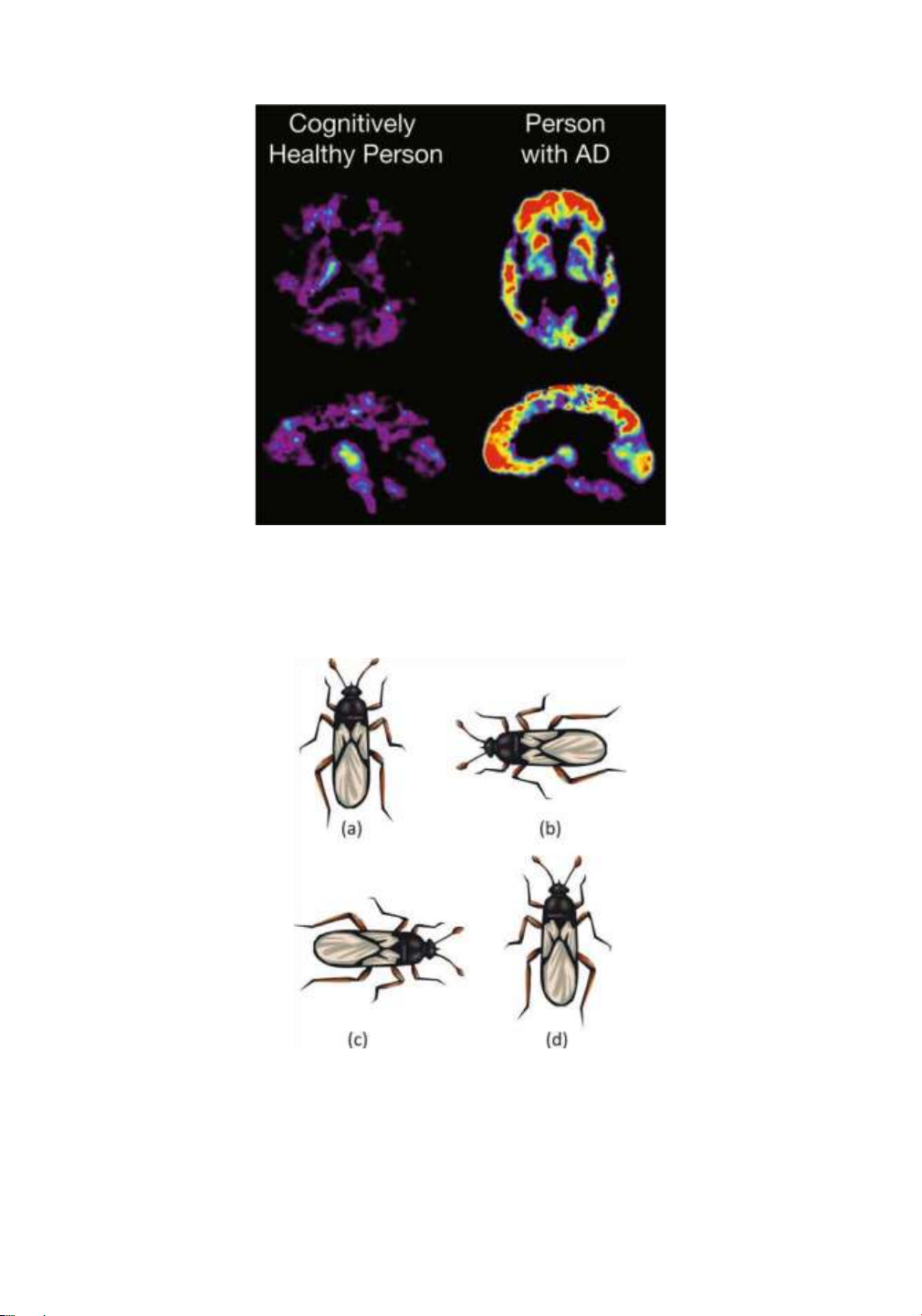
5. Medical diagnostics: Magnetic resonance imaging (MRI) and positron emission
tomography (PET) scans are spatial data in 2 or 3 dimensions. The detection of unusual
C. C. Aggarwal, Data Mining: The Textbook, DOI 10.1007/978-3-319-14142-8 16 531
c Springer International Publishing Switzerland 2015
localized regions in such data can help in detecting diseases such as brain tumors, the
onset of Alzheimer disease, and multiple sclerosis lesions. In general, any form of image lOMoAR cPSD| 59735516 532
CHAPTER 16. MINING SPATIAL DATA
data may be considered spatial data. The analysis of shapes in such data is of
considerable importance in a variety of applications.
6. Demographic data: Demographic (behavioral) attributes such as age, sex, race, and salary
can be combined with spatial (contextual) attributes to provide insights about the
demographic patterns in distributions. Such information can be useful for targetmarketing applications.
Most forms of spatial data may be classified as a contextual data type, in which the attributes
are partitioned into contextual attributes and behavioral attributes. This partitioning is
similar to that in time series and discrete sequence data:
• Contextual attribute(s): These represent the attributes that provide the context in which
the measurements are made. In other words, the contextual attributes provide the
reference points at which the behavioral values are measured. In most cases, the
contextual attributes contain the spatial coordinates of a data point. In some cases, the
contextual attribute might be a logical location, such as a building or a state. In the case
of spatiotemporal data, the contextual attributes may include time. For example, in an
application in which the sea surface temperatures are measured at sensors at specific
locations, the contextual attributes may include both the position of the sensor, and the
time at which the measurement is made.
• Behavioral attribute(s): These represent the behavioral values at the reference points.
For example, in the aforementioned sea surface temperature application, these
correspond to the temperature attribute values.
In most forms of spatial data, the spatial attributes are contextual, and may optionally include
temporal attributes. An exception is the case of trajectory data, in which the spatial attributes
are behavioral, and time is the only contextual attribute. In fact, trajectory data can be
considered equivalent to multivariate time series data. This equivalence is discussed in greater detail in Sect. 16.3.
This chapter separately studies cases where the spatial attributes are contextual, and those
in which the spatial attributes are behavioral. The latter case typically corresponds to
trajectory data, in which the contextual attribute corresponds to time. Thus, trajectory data is
a form of spatiotemporal data. In other forms of spatiotemporal data, both spatial and
temporal attributes are contextual.
This chapter is organized as follows. Section 16.2 addresses data mining scenarios in which
the spatial attributes are contextual. In this context, the chapter studies several important
problems, such as pattern mining, clustering, outlier detection, and classification. Section 16.3
discusses algorithms for mining trajectory data. Section 16.4 discusses the summary. 16.2
Mining with Contextual Spatial Attributes
In many forms of meteorological data, a variety of (behavioral) attributes, such as temperature,
pressure, and humidity, are measured at different spatial locations. In these cases, the spatial
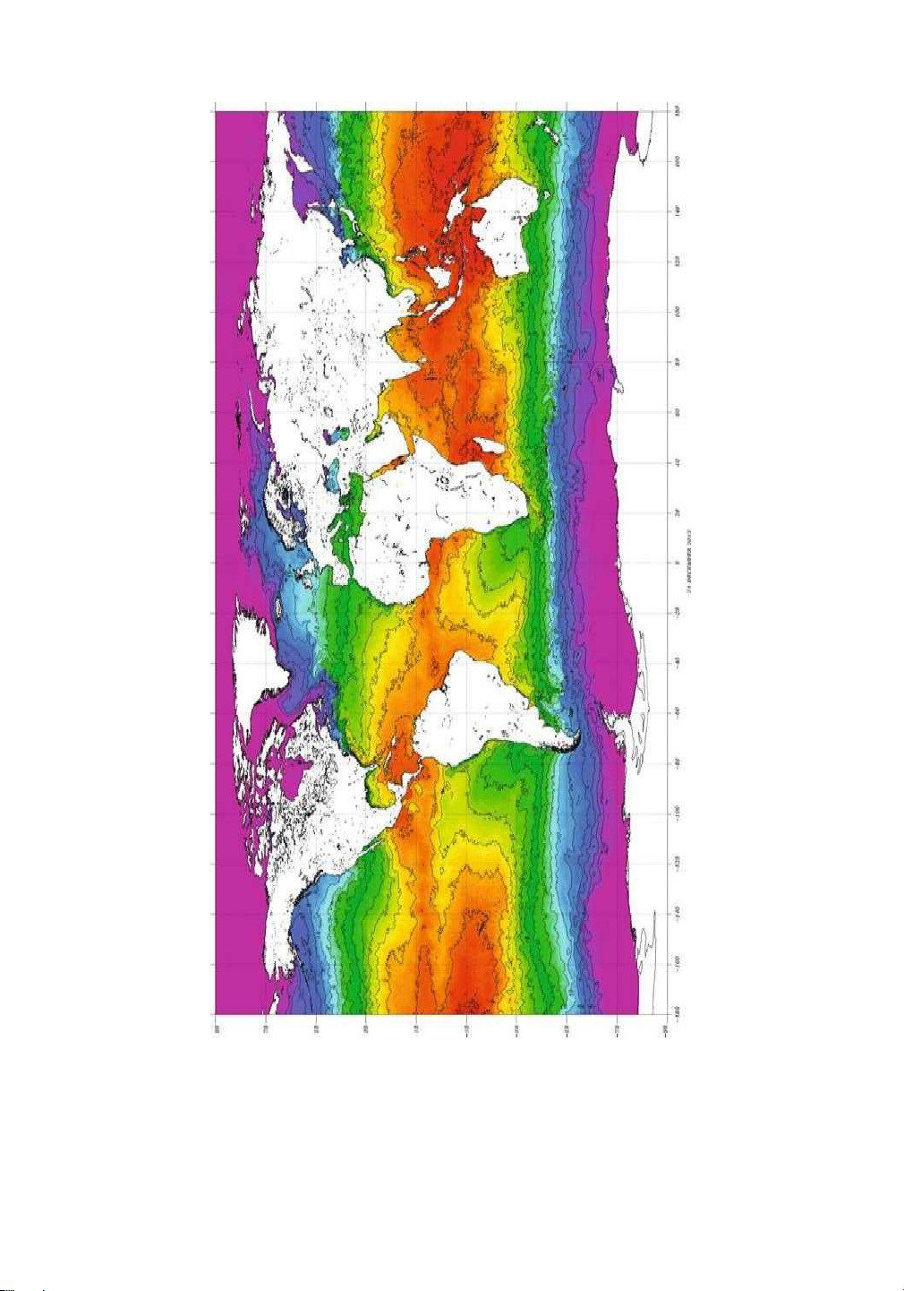
attributes are contextual. An example of sea surface temperature contour charts is illustrated
in Fig. 16.1. The different shades in the chart represent the different sea surface temperatures.
These correspond to the values of the behavioral attributes at different spatial locations.
Another example is the case of image data, where the intensity of an image is measured in
pixels. Such data is often used to capture diagnostic images. Examples of PET scans for a lOMoAR cPSD| 59735516
16.2. MINING WITH CONTEXTUAL SPATIAL ATTRIBUTES 533
cognitively healthy person and an Alzheimer’s patient are illustrated in Fig. 16.2. In this case,
the values of the pixels represent the behavioral attributes, and the spatial locations of these
pixels represent the contextual attributes. The behavioral attributes in spatial data may
present themselves in a variety of ways, depending on the application domain:
1. For some types of spatial data, such as images, the analysis may be performed on
thecontour of a specific shape extracted from the data. For example, in Fig. 16.3, the
contour of the insect may be extracted and analyzed with respect to other images in the data.
2. For other types of spatial data, such as meteorological applications, the
behavioralattributes may be abstract quantities such as temperature. Therefore the
analysis can be performed in terms of the trends on these abstract quantities. In such
cases, the spatial data needs to be treated as a contextual data type with multiple
reference points corresponding to spatial coordinates. Such an analysis is generally more complex.
The specific choice of data mining methodology often depends on the application at hand. Both
these forms of data are often transformed into other data types such as time series or
multidimensional data before analysis. 16.2.1
Shape to Time Series Transformation
In many spatial data sets such as images, the data may be dominated by a particular shape.
The analysis of such shapes is challenging because of the variations in sizes and orientations.
One common technique for analyzing spatial data is to transform it into a different format that
is much easier to analyze. In particular, the contours of a shape are often transformed to time
series for further analysis. For example, the contours of the insect shapes in Fig. 16.3 are
difficult to analyze directly because of their complexity. However, it is possible to create a
representation that is friendly to data processing by transforming them into time series.
A common approach is to use the distance from the centroid to the boundary of the object,
and compute a sequence of real numbers derived in a clockwise sweep of the boundary. This
yields a time series of real numbers, and is referred to as the centroid distance signature. This
transformation can be used to map the problem of mining shapes to that of mining time series.
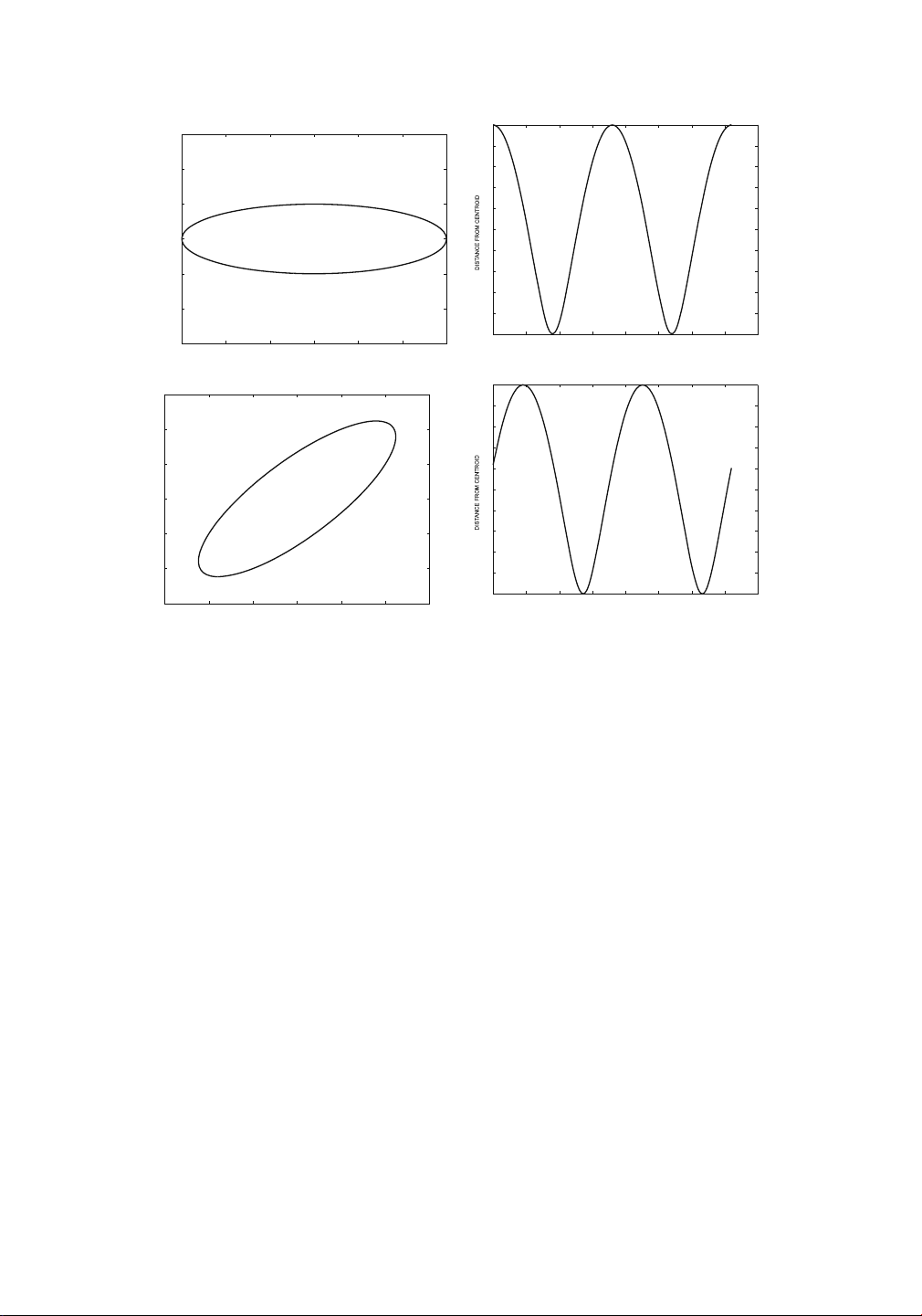
The latter domain is much easier to analyze. For example, consider the elliptical shape
illustrated in Fig. 16.4a. Then, the time series representing the distance from the centroid,
using 360 different equally spaced angular samples, is illustrated in Fig. 16.4b. Note that the
contextual attribute here is the number of degrees, but one can “pretend” that this represents
a timestamp. This facilitates the use of all the powerful data mining techniques available for
time series analysis. In this case, the sample points are started at one of the major axes of the
ellipse. If the sample point starts at a different position, or if the shape is rotated (with the
same angular starting point), then this causes a cyclic translation of the time series. This is
quite important because the precise orientation of a shape may not be known in advance. For
example, the shapes in Figs. 16.3b and c are rotated from the lOMoAR cPSD| 59735516 534
CHAPTER 16. MINING SPATIAL DATA
Figure 16.1: Contour charts for sea surface temperatures: Image courtesy of the NOAA Satellite and Information Service lOMoAR cPSD| 59735516
16.2. MINING WITH CONTEXTUAL SPATIAL ATTRIBUTES 535
Figure 16.2: PET Scans of the brain of a cognitively healthy person versus an Alzheimer’s
patient. (Image courtesy of the National Institute on Aging/National Institutes of Health)
Figure 16.3: Rotation and mirror image effects on shape matching lOMoAR cPSD| 59735516 536
CHAPTER 16. MINING SPATIAL DATA 3 3 2.8 2 2.6 2.4 1 2.2 2 0 1.8 −1 1.6 1.4 −2 1.2 1 0 50 100 150 200 250 300 350 400 −3 −3 −2 −1 0 1 2 3 DEGREES FROM START OF SWEEP (a )ellipticalshape (b )distancefromcentroidfor(a ) 3 3 2.8 2 2.6 2.4 1 2.2 2 0 1.8 −1 1.6 1.4 −2 1.2 1 0 50 100 150 200 250 300 350 400 −3 −3 −2 −1 0 1 2 3 DEGREES FROM START OF SWEEP (c) elliptical shape
(d) distance from centroid for (c)
Figure 16.4: Conversion from shapes to time series
shape of Fig. 16.3a. The shape in Fig. 16.3d is a mirror image of the shape of Fig. 16.3a. While
rotations result in cyclic translations, mirror images result in a reversal of the series.
Figure 16.4c represents a rotation of the shape of Fig. 16.4a by 45◦. Correspondingly, the
time series representation in Fig. 16.4d is a (cyclic) translation of time series representation
in Fig. 16.4b. Similarly, the mirror image of a shape corresponds to a reversal of the time series.
It will be evident later that the impact of rotation or mirror images needs to be explicitly
incorporated into the distance or similarity function for the application at hand. After the time
series has been extracted, it may be normalized in different ways, depending on the needs of the application:
• If no normalization is performed, then the data mining approach is sensitive to the
absolute sizes of the underlying objects. This may be the case in many medical images
such as MRI scans, in which all spatial objects are drawn to the same scale.
• If all time series values are multiplicatively scaled down by the same factor to unit mean,
such an approach will allow the matching of shapes of different sizes, but discriminate
between different levels of relative variations in the shapes. For example, two ellipses
with very different ratios of the major and minor axes will be discriminated well.
• If all time series are standardized to zero mean and unit variance, then such an approach
will match shapes where relative local variations in the shape are similar, but the overall
shape may be quite different. For example, such an approach will not discriminate very
well between two ellipses with very different ratios of the major and minor axes, but
will discriminate between two such shapes with different relative local deviations in the lOMoAR cPSD| 59735516
16.2. MINING WITH CONTEXTUAL SPATIAL ATTRIBUTES 537
boundaries. The only exception is a circular shape that appears as a straight line.
Furthermore, noise effects in the contour will be differentially enhanced in shapes that
are less elongated. For example, for two ellipses with similar noisy deviations at the
boundaries, but different levels of elongation (major to minor axis ratio), the overall
shape of the time series will be similar, but the local noisy deviations in the extracted
time series will be differentially suppressed in the elongated shape. This can sometimes
provide a distorted picture from the perspective of shape analysis. A perfectly circular
shape may show unstable and large noisy deviations in the extracted time series
because of trivial variations such as image rasterization effects. Thus, the usual mean
and variance normalization of time series analysis often leads to unintended results.
In general, it is advisable to select the normalization method in an application-specific way.
After the shapes have been converted to time series, they can be used in the context of a wide
variety of applications. For example, motifs in the time series correspond to frequent contours
in the spatial shapes. Similarly, clusters of similar shapes may be discovered by determining
clusters in the time series. Similar observations apply to the problems of outlier detection and classification. 16.2.2
Spatial to Multidimensional Transformation with Wavelets
For data types such as meteorological data in which behavioral attribute values vary across
the entire spatial domain, a contour-based shape may not be available for analysis. Therefore,
the shape to time series transformation is not appropriate in these cases.
Wavelets are a popular method for the transformation of time series data to
multidimensional data. Spatial data shares a number of similarities with time series data. Time
series data has a single contextual attribute (time) along which a behaviorial attribute (e.g.,
temperature) may exhibit a smooth variation. Correspondingly, spatial data has two
contextual attributes (spatial coordinates), along which a behavioral attribute (e.g., sea
surface temperature) may exhibit a smooth variation. Because of this analogy, it is possible to
generalize the wavelet-based approach to the case of multiple contextual attributes with appropriate modifications.
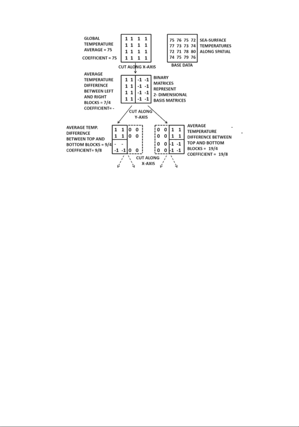
Assume that the spatial data is represented in the form of a 2-dimensional grid of size q×q.
Thus, each coordinate of the grid contains an instance of the behavioral attribute, such as the
temperature. As discussed for the time series case in Sect. 2.4.4.1 of Chap. 2, differencing
operations are applied over contiguous segments of the time series by successive division of
the time series in hierarchical fashion. The corresponding basis vectors have +1 and −1 at the
relevant positions. The 2-dimensional case is completely analogos, where contiguous areas of
the spatial grid are used for successive divisions. These divisions are alternately performed
along the different axes. The corresponding basis vectors are 2-dimensional matrices of size q
× q that regulate how the differencing operations are performed. An example of how sea
surface temperatures in a spatial data set may be converted to a multidimensional
representation is provided in Fig. 16.5. This will result in a total of q2 wavelet coefficients,
though only the large coefficients need to be retained for analysis. A more detailed description
of the generation of the spatial wavelet coefficients may be found in Sect. 2.4.4.1 of Chap. 2.
The aforementioned description is for the case of a single behavioral attribute and multiple
contextual attributes (spatial coordinates). Multiple behavioral attributes can also lOMoAR cPSD| 59735516 538
CHAPTER 16. MINING SPATIAL DATA GRID 7/8 1 1 0 0 Figure 16.5: Illustration of the top
levels of the wavelet decomposition for spatial data in a grid containing sea surface
temperatures (Fig. 2.7 of Chap. 2 revisited)
be addressed by performing the decomposition separately for each behavioral attribute, and
creating a separate set of dimensions for each behavioral attribute.
Like the time series wavelet, the spatial wavelet is a multiresolution representation.
Trends at different levels of spatial granularity are represented in the coefficients. Higherlevel
coefficients represent trends in larger spatial areas, whereas lower-level coefficients
represent trends in smaller spatial areas. Therefore, this approach is very powerful, and has
broad usability for many spatial applications. Spatial wavelets can be used effectively for many
image clustering and classification applications where (contextual) spatial data can be
converted to (noncontextual) multidimensional data. Once the transformation has been
performed, virtually all the multidimensional methods discussed in Chaps. 4 to 11 can be used
on this representation. Such an approach opens the door to the use of a wide array of
multidimensional data mining methods. 16.2.3
Spatial Colocation Patterns
In this problem, the contextual attributes are spatial and the behavioral attributes are typically
boolean and nonspatial. Non-boolean behavioral attributes can be addressed with the use of
type conversion via discretization or binarization. The goal of spatial colocation pattern
mining is to discover combinations of features occurring at the same spatial location. Consider
an ecology data set, where one has behavioral attributes such as fire ignition source, needle
vegetation type, and a drought indicator. The spatial colocation of these features may often be
a risk factor for forest fires. Therefore, the discovery of such patterns is useful in the context
of data mining analysis. In many cases, a spatial event indicator of interest (e.g., disease
outbreak, vegetation event, or climate event) is added to the other behavioral attributes. The
discovery of useful patterns that include this indicator of interest can be used for discovering
event causality. This problem is also closely related to rule-based spatial classification, where
the likelihood of the event occurring in previously unseen test regions can be estimated from the resulting patterns. lOMoAR cPSD| 59735516
16.2. MINING WITH CONTEXTUAL SPATIAL ATTRIBUTES 539
One challenge in the mining process is that the different behavioral attributes may be
derived from different data sources, and therefore may not have precisely the same value of
the contextual (spatial) attribute in their measurements. Therefore, proper data
preprocessing is crucial. The data can be homogenized by partitioning the spatial region into
smaller regions. For each of these regions, each behavioral attribute’s value is derived
heuristically from the values in the original data source. For example, if the boolean attribute
has a value of 1 more than predefined fraction of the time in a spatial region, then its value is
set to 1. The contextual (spatial) attribute can be set to the centroid of that region. The mining
can be performed on this preprocessed data. The overall approach is as follows:
1. Preprocess the data to create the behavioral attribute values at the same set of spatiallocations.
2. For each spatial location, create a transaction containing the corresponding
combination of boolean values.
3. Use any frequent pattern mining algorithm to discover the relevant patterns in these transactions.
4. For each discovered pattern, map it back to the spatial regions containing the
pattern.Cluster the relevant spatial regions for each pattern, if necessary for summarization.
In cases where a particular behavioral attribute is an event of interest (e.g., disease outbreak),
the transactions containing values of 0 and 1, respectively, for this attribute can be separately
processed to discover two sets of patterns on the other behavioral attributes. The differences
between these two sets of patterns can provide insights into discriminative factors for the
event of interest at each spatial location. Such patterns are also useful for spatial classification
of previously unseen test regions. This approach is identical to that of associative classifiers in Chap. 10.
This model can also address time-changing data in a seamless way. In such cases, the time
becomes another contextual attribute in addition to the spatial attributes. Patterns can be
discovered at different temporal snapshots using the aforementioned methodology. The key
changes in these patterns over time can provide insights into the nature of the spatial evolution. 16.2.4 Clustering Shapes
In many applications, it may be desirable to cluster similar shapes prior to analysis. It is
assumed that a database of N shapes is available and that a total of k groups of similar shapes
need to be created. This can be a useful preprocessing task in many shape categorization
applications. The conversion of a shape to a time series (Sect. 16.2.1) is the appropriate
approach in this scenario. Many of the time series clustering algorithms discussed in Sect. 14.5
of Chap. 14 may be used effectively, once the shape has been converted to a time series. The k-
medoids, hierarchical, and graph-based methods are particularly suitable because they
require only the design of an appropriate similarity function for the corresponding time series.
This is an issue that will be discussed in more detail later. The main steps of shape-based clustering are as follows:
1. Use the centroid-based sweep method discussed in Sect. 16.2.1 to convert each shape
into a time series. This results in a database of N different time series. lOMoAR cPSD| 59735516 540
CHAPTER 16. MINING SPATIAL DATA
2. Use any time series clustering algorithm, such as hierarchical, k-medoids or graphbased
method on time series data as discussed in Sect. 14.5 of Chap. 14. This will cluster the N
time series into k groups.
3. Map the k groups of time series clusters to k groups of shape clusters, by mapping each
time series into its relevant shape.
The aforementioned clustering algorithm depends only on the choice of the distance function.
Any of the time series measures discussed in Sect. 3.4.1 of Chap. 3 may be used, depending on
the desired degree of error tolerance or distortion (warping) allowed in the matching. Another
important issue is the adjustment of the distance function with the varying rotations of the
different shapes. In the following, the Euclidean distance will be used as an example, although
the general principle can be applied to any distance function.
It is evident from the example of Fig. 16.4 that a rotation of the shape leads to a linear cyclic
shifting of the time series generated by using the distances of the centroid of the shape to the
contours of the shape. For a time series of length n denoted by a1a2 ...an, a cyclic translation by
i units leads to the time series ai+1ai+2 . .ana1a2 . .ai. Then, the rotation invariant Euclidean
distance RIDist(T1,T2) between two time series T1 = a1 ...an and T2 = b1 . .bn is given by the
minimum distance between T1 and all possible rotational translations of T2 (or vice versa).
Therefore, the rotation-invariant distance is expressed as follows: n
RIDist ( T 1 ,T 2 )= min n i =1
( a j − b 1+( j + i ) mod n ) 2 j =1 .
In general, if a cyclic shift of the time series T T i
2 by i units is denoted by 2 , then the rotation
invariant distance, using any distance function Dist(T1,T2) may be expressed as follows:
RIDist ( T 1 ,T 2 )= min n i =1 Dist ( T 1 ,T i 2 ). (16.1)
Note that the reversal of a time series corresponds to the mirror image of the underlying shape.
Therefore, mirror images can also be addressed using this approach, by incorporating the
reversals of the series (and its rotations) in the distance function. This will increase the
computation by a factor of 2. The precise choice of distance function used is highly application-
specific, depending on whether rotations or mirror image conversions are required. 16.2.5 Outlier Detection
In the context of spatial data, outliers can be either point outliers and shape outliers. These
two kinds of outliers are also encountered in time series data, and in discrete sequences. In
the case of spatial data, these two kinds of outliers are defined as follows:
1. Point outliers: These outliers are defined on a single spatial object with a variety of
spatial and behavioral attributes. For example, a weather map is a spatial object that
contains both spatial locations, and environmental measurements (behavioral values)
at these locations. Abrupt changes in the behavioral attributes that violate spatial
continuity provide useful information about the underlying contextual anomalies. For
example, consider a meteorological application in which sea surface temperatures and lOMoAR cPSD| 59735516
16.2. MINING WITH CONTEXTUAL SPATIAL ATTRIBUTES 541
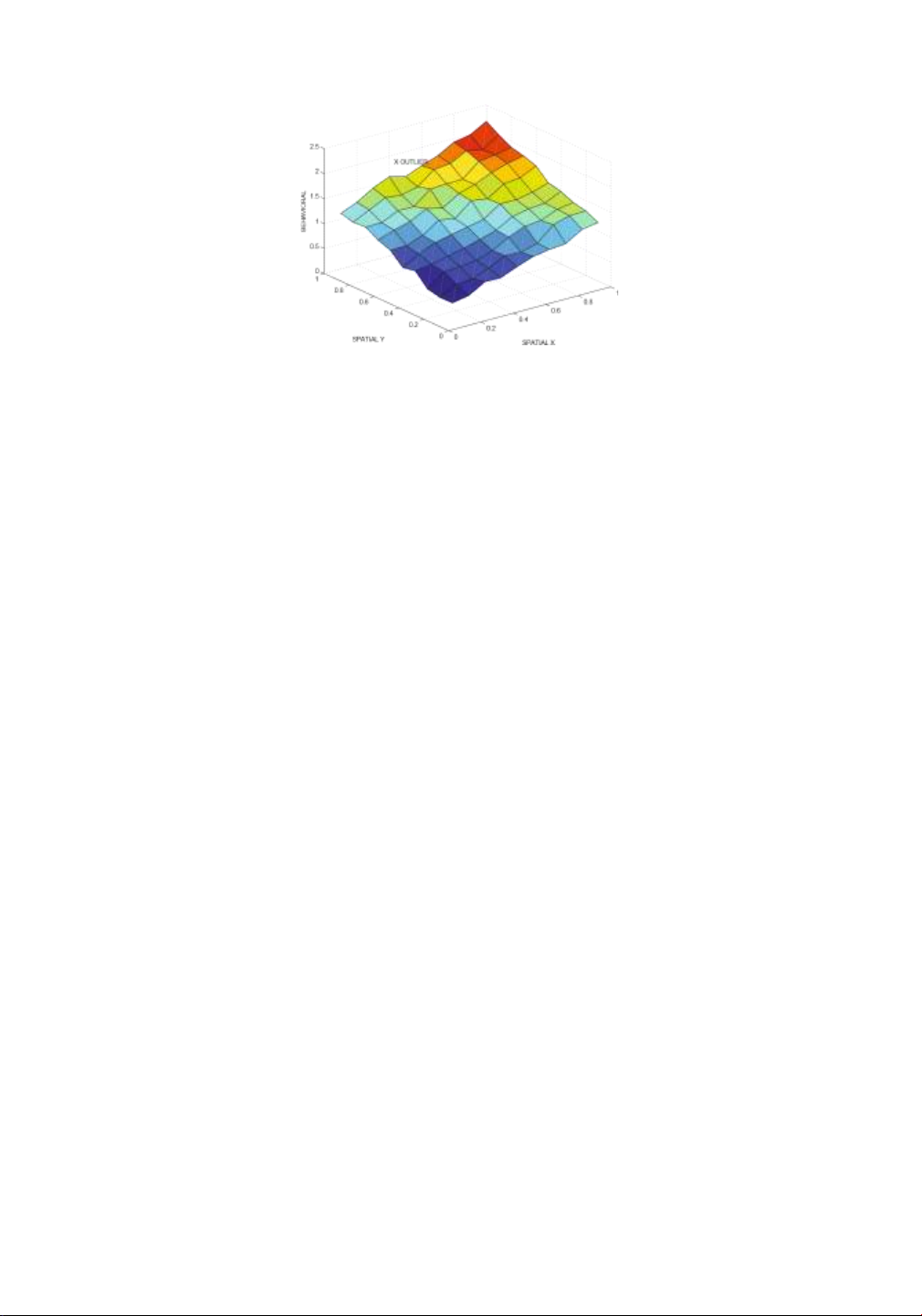
Figure 16.6: Example of point outlier for spatial data
pressure are measured. Unusually high sea surface temperature in a very small localized
region is a hot-spot that may be the result of volcanic activity under the surface. Similarly,
unusually low or high pressure in a small localized region may suggest the formation of
hurricanes or cyclones. In all these cases, spatial continuity is violated by the attribute
of interest. Such attributes are often tracked in meteorological applications on a daily
basis. An example of a point outlier for spatial data is illustrated in Fig. 16.6.
2. Shape outliers: The application settings for these kinds of outliers are quite different.
These outliers are defined in a database of multiple shapes. For example, the shapes
may be extracted from the different images. In such cases, the unusual shapes in the
different objects need to be reported as outliers.
This chapter studies both the aforementioned formulations. 16.2.5.1 Point Outliers
Neighborhood-based algorithms are generally used for discovering point outliers. In these
algorithms, abrupt changes in the spatial neighborhood of a data point are used to diagnose
outliers. Therefore, the first step is to define the concept of a spatial neighborhood. The
behavioral values within the spatial neighborhood of a given data point are combined to create
an expected value of the behavioral attribute. This expected value is then used to compute the
deviation of the data point from the expected value. This provides an outlier score. This
definition of point outliers in spatial data is similar to that in time series data.
Intuitively, it is unusual for the behavioral attribute value to vary abruptly within a small
spatial locality. For example, a sudden variation of the temperature within a small spatial
locality will be detected by this method. The neighborhood may be defined in many different ways:
• Multidimensional neighborhoods: In this case, the neighborhoods are defined with the
use of multidimensional distances between data points. This approach is appropriate
when the contextual attributes are defined as coordinates.
• Graph-based neighborhoods: In this case, the neighborhoods are defined by linkage
relationships between spatial objects. Such neighborhoods may be more useful in cases
where the location of the spatial objects may not correspond to exact coordinates (e.g.,
county or ZIP code). In such cases, graph-based representations provide a more general modeling tool. lOMoAR cPSD| 59735516 542
CHAPTER 16. MINING SPATIAL DATA
Both multidimensional and graph-based methods will be discussed in the following sections.
Multidimensional Methods
While traditional multidimensional methods can also be used to detect outliers in spatial data,
such methods do not distinguish between the contextual and the behavioral attributes.
Therefore, such methods are not optimized for outlier detection in spatial data. This is because
the (contextual) spatial attributes should be treated differently from the behavioral attributes.
The basic idea is to adapt the k-nearest neighbor outlier detection methods to the case of spatial data.
The spatial neighborhood of the data is defined with the use of multidimensional distances
on the spatial (contextual) attributes. Thus, the contextual attributes are used for determining
the k nearest neighbors. The average of the behavioral attribute values provides an expected
value for the behavioral attribute. The difference between the expected and true value is used
to predict outliers. A variety of distance functions can be used on the multidimensional spatial
data for the determination of proximity. The choice of the distance function is important
because it defines the choice of the neighborhood that is used for computing the deviations in
behavioral attributes. For a given spatial object o, with behavioral attribute value f(o), let o1 ...ok
be its k-nearest neighbors. Then, a variety of methods may be used to compute the predicted
value g(o) of the object o. The most straightforward method is the mean: k g ( o )=
f ( o i) /k i =1
Alternatively, g(o) may be computed as the median of the surrounding values of f(oi), to reduce
the impact of extreme values. Then, for each data object o, the value of f(o) − g(o) represents
a deviation from predicted values. The extreme values among these deviations may be
computed using a variety of methods for univariate extreme value analysis. These are
discussed in Chap. 8. The resulting extreme values are reported as outliers. Graph-Based Methods
In graph-based methods, spatial proximity is modeled with the use of links between nodes in
a graph representation of the spatial region. Thus, nodes are associated with behavioral
attributes, and strong variations in the behavioral attribute across neighboring nodes are
recognized as outliers. Graph-based methods are particularly useful when the individual
nodes are not associated with point-specific coordinates, but they may correspond to regions
of arbitrary shape. In such cases, the links between nodes correspond to neighborhood
relationships between the different regions. Graph-based methods define spatial
relationships in a more general way because semantic relationships can also be used to define
neighborhoods. For example, two objects could be connected by an edge if they are in the same
semantic location, such as a building, restaurant, or an office. In many applications, the links
may be weighted on the basis of the strength of the proximity relationship. For example,
consider a disease outbreak application in which the spatial objects correspond to county
regions. In such a case, the strength of the links could correspond to the length of the boundary
between two regions. Multidimensional data is a special case, where links correspond to
distance-based proximity. Thus, graph representations allow more generic interpretations of the contextual attribute.
Let S be the set of neighbors of a given node i. Then, the concept of spatial continuity can
be used to create a predicted value of the behavioral attribute based on those of its (spatial)
neighbors. The strength of the links between i and its neighbors can also be used to compute
the predicted values as either the weighted mean or median on the behavioral attribute of the lOMoAR cPSD| 59735516
16.2. MINING WITH CONTEXTUAL SPATIAL ATTRIBUTES 543
k nearest spatial neighbors. For a given spatial object o with the behavioral attribute value f(o),
let o1 ...ok be its k linked neighbors based on the relationship graph. Let the weight of the link
(o,oi) be w(o,oi). Then, the linkage-based weighted mean may be used to compute the predicted
value g(o) of the object o. k g ( o )=
i =1 w ( o,o i ) · f ( o i )
k i =1 w ( o,o i )
Alternatively, the weighted median of the neighbor values may be used for predictive purposes.
Since the true value of the behavioral attribute is known, this can be used to model the
deviations of the behavioral attributes from their predicted values. As in the case of
multidimensional methods, the value of f(o) − g(o) represents a deviation from the predicted
values. Extreme value analysis can be used on these deviations to determine the spatial
outliers. This process is identical to that in the multidimensional case. The nodes with high
values of the normalized deviation may be reported as outliers. 16.2.5.2 Shape Outliers
Shape-based outliers are relatively easy to determine in spatial data, with the use of the
transformation from spatial data to time series described in Sect. 16.2.1. After the
transformation has been performed, a k-nearest neighbor outlier detector can be applied to
the resulting time series. The distance to the kth-nearest neighbor can be reported as the
outlier score. A few key issues need to be kept in mind, while computing the outlier score.
1. The distance function needs to be modified to account for the rotation invariance
ofshape matching. This is achieved by comparing all cyclic shifts of one time series to
the other. The rotation invariant distance can be captured by Eq. 16.1.
2. In some applications, mirror image invariance also needs to be accounted for. In such
cases, all cyclic shifts and their reversals need to be included in the aforementioned
comparison. The outliers are determined with respect to this enhanced database.
While a vanilla k-nearest neighbor detector can determine the outliers correctly, the approach
can be made faster by pruning. The basic idea is similar to the Hotsax method discussed in
Chap. 14, where a nested loop structure is used to maintain the top-n outliers. The outer loop
corresponds to the selection of different candidates, and the inner loop corresponds to the
computation of the k-nearest neighbors of each of these candidates. The inner loop can be
terminated early, when the k-nearest neighbor value is less than the nth best outlier found so
far. For optimal performance, the candidates in the outer loop and the computations in the
inner loop need to be ordered appropriately.
This ordering is performed as follows. A combination of the SAX representation and LSH-
hashing is used to create clusters on the candidates. Candidates which map to clusters with
few members are examined first in the outer loop to discover high quality outliers early in the
algorithm execution. Objects which appear in the same cluster as the outer loop candidate are
examined first in the inner loop to ensure fast termination of the inner loop. This facilitates
better pruning performance. The bibliographic notes contain pointers to specific details of the
creation of SAX-based clusters in shape outlier detection. 16.2.6
Classification of Shapes
It is assumed that a set of N labeled shapes are used to conduct the training. This trained model
is used to perform classification of test instances, for which the label is unknown. The
transformation from spatial into time series data is a useful tool for distance-based lOMoAR cPSD| 59735516 544
CHAPTER 16. MINING SPATIAL DATA
classification algorithms. As in the case of clustering and outlier detection, the first step of the
process is to transform the shapes into time series. This transforms the problem to the time
series classification problem. A number of methods for the classification of time series are
discussed in Sect. 14.7 of Chap. 14. The main difference is that the rotation invariance of the
shapes needs to be accounted for. Any of the distance-based methods proposed in Sect. 14.7
of Chap. 14 for time series classification may be used after the shapes have been transformed
into time series. This is because distance-based methods can be easily made rotation-invariant
by using Eq. 16.1. The two main distance-based methods for time series classification include
the nearest neighbor method and the graph-based collective classification approach. While
the nearest-neighbor method is straightforward, the graphbased method is discussed in some detail below.
The graph-based method is transductive because it requires the test instances to be
available at the time of training. When a larger number of test instances are available along
with the training data, the latter method may be used. Therefore, the different methods may
be more suitable in different scenarios. The overall approach for graph-based classification may be described as follows:
1. Transform both the training and test shapes into time series, by using the centroidsweep
method described in Sect. 16.2.1.
2. Use any of the distance functions described in Sect. 3.4.1 of Chap. 3 to construct a
neighborhood graph on the shapes. If needed, use a rotation-invariant version of the
distance function, as discussed in Eq. 16.1. Each shape represents a node, which is
connected to its k-nearest neighbors with edges. The labeled shapes correspond to
labeled nodes. The collective classification method described in Sect. 19.4 of Chap. 19 is
used to assign labels to the unlabeled nodes (i.e., the test shapes).
In some cases, rotation invariance may not be an application-specific need. In such cases, the
efficiency of distance computation is improved. 16.3 Trajectory Mining
Trajectory data arises in a wide variety of spatial applications. The proliferation of GPSenabled
devices, such as mobile phones, has enabled the large-scale collection of trajectory data.
Trajectory data can be analyzed for a very wide variety of insights, such as determining co-
location patterns, clusters and outliers. Trajectory data is different from the other kinds of
spatial data discussed in this chapter in the following respects:
1. In the spatial data applications addressed so far in this chapter, spatial attributesare
contextual, whereas other types of attributes (e.g., temperature in a meteorological
application) are behavioral. In the case of trajectory data, spatial attributes are behavioral. lOMoAR cPSD| 59735516 16.3. TRAJECTORY MINING 545
2. The only contextual attribute in trajectory data is time. Therefore, trajectory data can be
considered spatiotemporal data. While the scenarios discussed in previous sections may
also be generalized further by including time among the contextual attributes, the
spatial attributes are not behavioral in those cases. For example, when sea surface
temperatures are tracked over time, both spatial and temporal attributes are contextual.
Trajectory analysis is typically performed in one of two different ways:
1. Online analysis: In online analysis, the trajectories are analyzed in real time, and the
patterns in the trajectories at a given time are most relevant to the analysis.
2. Shape-based analysis: In shape-based analysis, the time variable has already been
removed from the analysis. For example, two similar trajectories, formed at different
periods, can be meaningfully compared to one another. For example, a cluster of
trajectories is based on their shape, rather than the simultaneity in their movement.
The two kinds of analysis in trajectory data are similar to time series data. This is not
particularly surprising because trajectory data is a form of time series data. 16.3.1
Equivalence of Trajectories and Multivariate Time Series
Trajectory data is a form of multivariate time series data. For a trajectory in two dimensions,
the X-coordinate and Y -coordinate of the trajectory form two components of the multivariate
series. A 3-dimensional trajectory will result in a trivariate series.
Because of the equivalence between multivariate time series and trajectory data, the
transformation can be performed in either direction to facilitate the use of the methods
designed for each domain. For example, trajectory mining methods can be utilized for
applications that are nonspatial. In particular, any n-dimensional multivariate time series can
be converted into trajectory data. In multivariate temporal data, the different behavioral
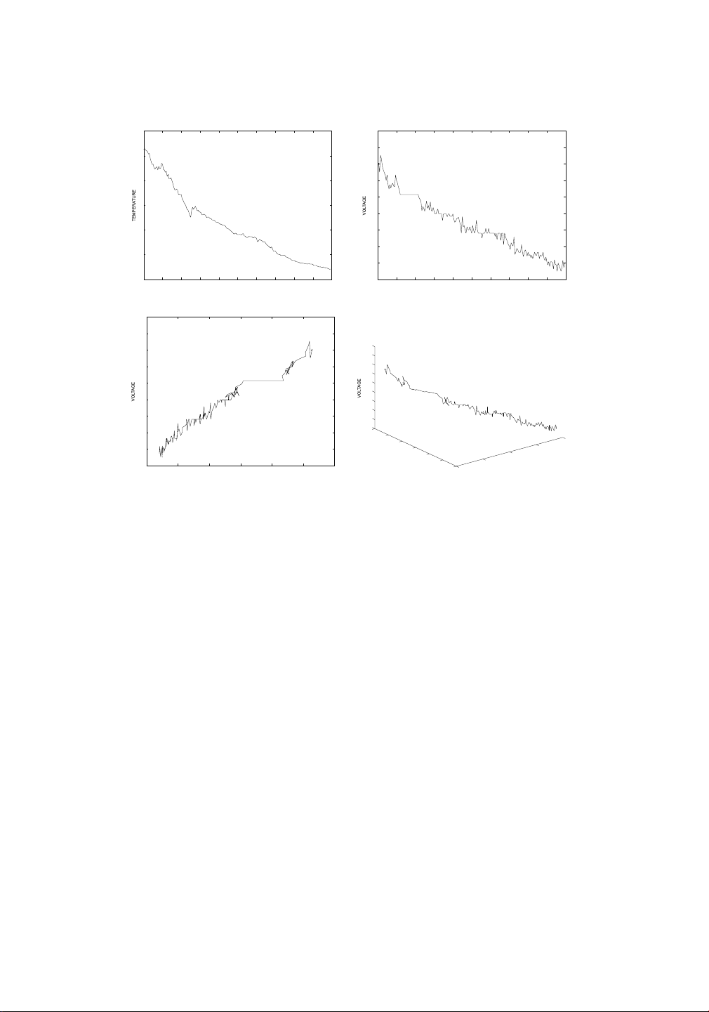
attributes are typically measured with the use of multiple sensors simultaneously. Consider
the example of the Intel Research Berkeley Sensor data [556] that measures different
behavioral attributes, such as temperature, pressure, and voltage, in the Intel Berkeley
laboratory over time. For example, the behavior of the temperature and voltage sensors in the
same segment of time are illustrated in Figs. 16.7a, b, respectively.
It is possible to visualize the variation of the two behaviorial attributes by eliminating the
common time attribute, or by creating a 3-dimensional trajectory containing the time and the
other two behaviorial attributes. Examples of such trajectories are illustrated in Fig. 16.7c, d,
respectively. The most generic of these trajectories is illustrated in Fig. 16.7d. This figure
shows the simultaneous variation of all three attributes. In general, a multivariate time series
with n behavioral attributes can be mapped to an (n + 1)-dimensional trajectory. Most of the
trajectory analysis methods are designed under the assumption of 2 or 3 dimensions, though
they can be generalized to n dimensions where needed. 16.3.2
Converting Trajectories to Multidimensional Data
Because of the equivalence between trajectories and multivariate time series, trajectories can
also be converted to multidimensional data. This is achieved by using the wavelet
transformation on the time series representation of the trajectory. The wavelet
transformation for time series is described in detail in Sect. 2.4.4.1 of Chap. 2. In this case, the lOMoAR cPSD| 59735516 546
CHAPTER 16. MINING SPATIAL DATA
time series is multivariate, and therefore has two behavioral attributes. The wavelet representation for 25 2.69 2.68 24 2.67 23 2.66 2.65 22 2.64 21 2.63 2.62 20 2.61 19 2.6 2000 2020 2040 2060 2080 2100 2120 2140 2160 2180 2200 2000 2020 2040 2060 2080 2100 2120 2140 2160 2180 2200 TIME STAMP TIME STAMP (a )Temperature (b )Voltage 2.69 2.68 2.69 2.67 2.68 2.67 2.66 2.66 2.65 2.65 2.64 2.64 2.63 2.62 2.63 2.61 2.6 2.62 25 24 23 22 2200 2.61 21 2150 20 2100 2.6 TEMPERATURE 19 20 21 22 23 24 25 19 2050 2000 TEMPERATURE TIME STAMP ( c)Temperature-Voltage ( d)Time-Temperature-Voltage Trajectory Trajectory
Figure 16.7: Multivariate time series can be mapped to trajectory data
each of these behavioral attributes is extracted independently. In other words, the time series
on the X-coordinate is converted into a wavelet representation, and so is the time series on
the Y -coordinate. This yields two multidimensional representations, one of which is for the X-
coordinate, and the other is for the Y -coordinate. The dimensions in these two
representations are combined to create a single higher-dimensional representation for the
trajectory. If desired, only the larger wavelet coefficients may be retained to reduce the
dimensionality. The conversion of trajectory data to multidimensional data is an effective way
to use the vast array of multidimensional methods for trajectory analysis. 16.3.3
Trajectory Pattern Mining
There are many different ways in which the problem of trajectory pattern mining may be
formulated. This is because of the natural complexity of trajectory data that allows for multiple
ways of defining patterns. In the following sections, some of the common definitions of
trajectory pattern mining will be explored. These definitions are by no means exhaustive,
although they do illustrate some of the most important scenarios in trajectory analysis. lOMoAR cPSD| 59735516 16.3. TRAJECTORY MINING 547 16.3.3.1
Frequent Trajectory Paths
A key problem is that of determining frequent sequential paths in trajectory data. To
determine the frequent sequential paths from a set of trajectories, the first step is to convert
the multidimensional trajectory (with numeric coordinates) to a 1-dimensional discrete P Q R S T P Q R S T A A AP AQ AR AS AT B B BP BQ BR BS BT C C CP CQ CR CS CT D D DP DQ DR DS DT E E EP EQ ER ES ET (a) Trajectory (b) Relevant grid regions
Figure 16.8: Grid-based discretization of trajectories
sequence. Once this conversion has been performed, any sequential pattern mining algorithm
can be applied to the transformed data.
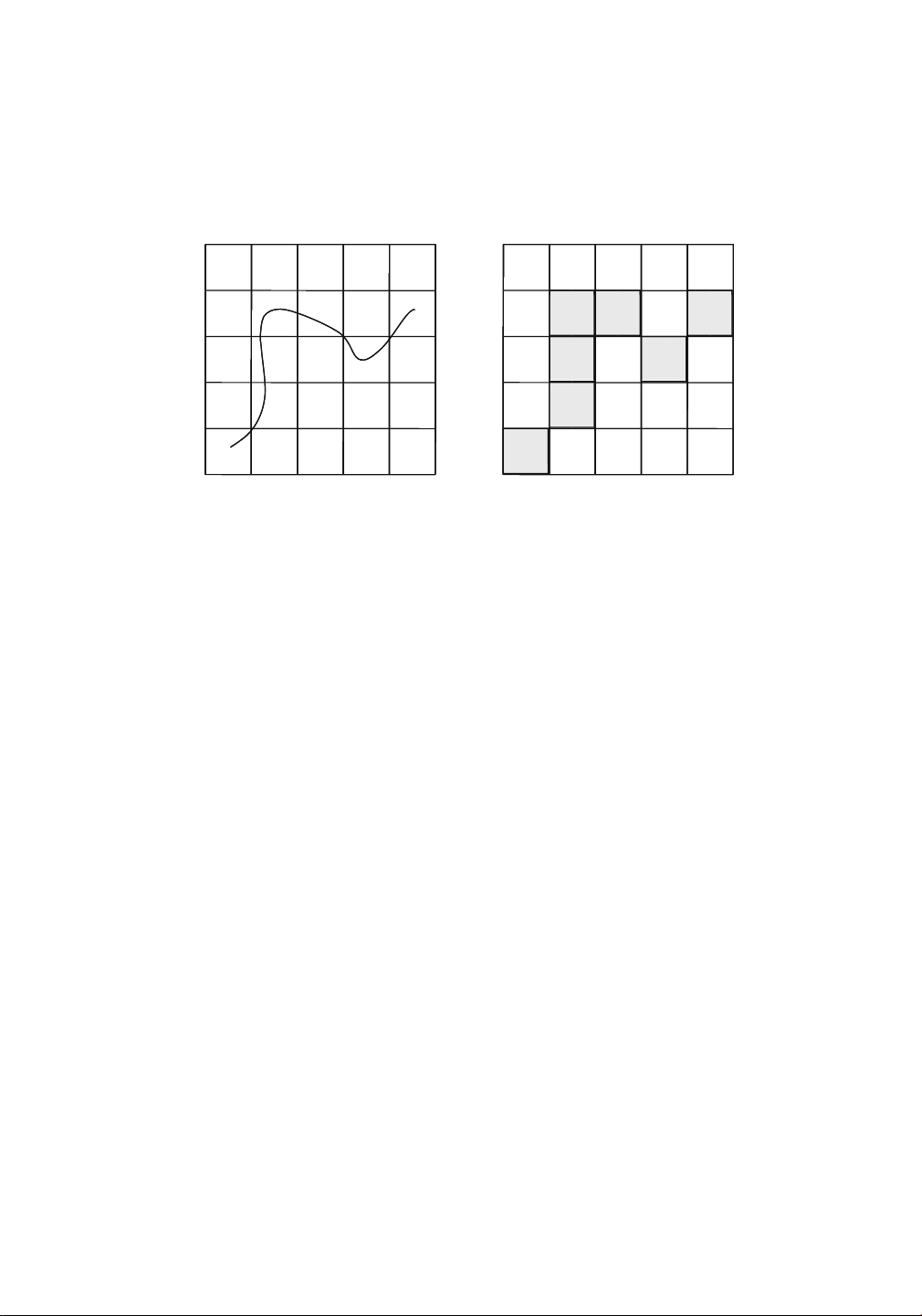
The most effective way to convert a multidimensional trajectory to a discrete sequence is
to use grid-based discretization. In Fig. 16.8a, a trajectory has been illustrated, together with
a 4×4 grid representation of the underlying data space. The grid ranges along one of the
dimensions are denoted by A, B, C, D, and E. The grid ranges along the other dimension are
denoted by P, Q, R, S, and T. The 2-dimensional tiles are denoted by a combination of the ranges
along each of the dimensions. For example, the tile AP represents the intersection of the grid
range A with the grid range P. Thus, each tile has a distinct (discrete) identifier, and a trajectory
can be expressed in terms of the sequence of discrete identifiers through which it passes. The
shaded tiles for the trajectory in Fig. 16.8a are illustrated in Fig. 16.8b. The corresponding 1-
dimensional sequential pattern is as follows: EP,DQ,CQ,BQ,BR,CS,BT
This transformation is referred to as the spatial tile transformation. In principle, it is possible
to enhance the discretization further, by imposing a minimum time spent in each grid square,
though this is not considered here. Consider a database containing N different trajectories.
The frequent sequential paths can be determined from these trajectories by using a two-step approach:
1. Convert each of the N trajectories into a discrete sequence, using grid-based discretization.
2. Apply the sequential pattern mining algorithms discussed in Sect. 15.2 of Chap. 15 to
discover frequent sequential patterns from the resulting data set. lOMoAR cPSD| 59735516 548
CHAPTER 16. MINING SPATIAL DATA
By incorporating different types of constraints on the sequential pattern mining process,
such as time-gap constraints, it is also possible to apply these constraints on the trajectories.
One advantage of this transformation-based approach is that it can take advantage of the
power of all the different variations of sequential pattern mining. Sequential pattern mining
has a rich body of literature on constraint-based methods.
Another interesting aspect is that this formulation can be modified to address situations
in which the patterns of movements occur at the same period in time. The time period over
which the movement occurs is discretized into m periods denoted by 1...m. For example, the
intervals could be [8AM,9AM], [9AM,10AM], [10AM,11AM], and so on. Thus, for each time-
interval, the grid identifier is tagged with the relevant time-period identifier. A time period
identifier is tagged to a grid region if a minimum amount of time from that time period range
was spent in that region by the trajectory. This results in a set of patterns defined on a new set
of discrete symbols of the form < GridId >:< TimeId >. In the trajectory of Fig. 16.8a, a possible
sequence that appends the time period identifier is as follows:
EP : 1,EP : 2,DQ : 2,DQ : 3,DQ : 4,CQ : 5,BQ : 5,BR : 5,CS : 6,CS : 7,BT : 7
This transformation is referred to as the spatiotemporal tile transformation. Note that this
sequence is longer than that in Fig. 16.8b because the trajectory may spend more than one
interval in the same grid region. A set of N different sequences are extracted, corresponding
to the N different trajectories. The sequential pattern mining can be performed on this new
representation. Because of the addition of the time identifiers, the resulting patterns will
correspond to simultaneous movements in time. Thus, the sequential pattern mining approach
has significant flexibility in terms of either detecting patterns of similar shapes, or patterns of
simultaneous movements. Furthermore, because the sequential pattern mining formulation
does not require successive symbols in a frequent sequential pattern to be contiguous in the
original sequence, it can ignore noisy gaps in the underlying trajectories, while mining
patterns. Furthermore, by using different constrained sequential pattern mining formulations,
different kinds of constrained trajectory patterns can be discovered.
One drawback of the approach is that the granularity level of the discretization may affect
the quality of the results. It is possible to address this issue by using a multigranularity
discretization of the spatial regions. A different approach for conversion to symbolic
representation is the use of spatial clustering on the different temporal snapshots of the object
positions. The cluster identifiers of each object over different snapshots may be used to
construct its sequence representation. The bibliographic notes contain pointers to several
algorithms for transformation and pattern discovery from trajectories. The broader idea of
many of these methods is to convert to a symbolic sequence representation for more effective pattern mining. 16.3.3.2 Colocation Patterns
Colocation patterns are designed to discover social connections between the trajectories of
different individuals. The basic idea of colocation patterns is that individuals who frequently
appear at the same point at the same time are likely to be related to one another. Colocation
pattern mining attempts to discover patterns of individuals, rather than patterns of spatial
trajectory paths. Because of the complementary nature of this analysis, a vertical
representation of the sequence database is particularly convenient. lOMoAR cPSD| 59735516 16.3. TRAJECTORY MINING 549
A similar grid discretization (as designed for the case of frequent trajectory patterns) can
be used for preprocessing. However, in this case, a somewhat different (vertical)
representation is used for the locations of the different individuals in the grid regions at
different times. For each grid region and time-interval pair, a list of person identifiers (or
trajectory identifiers) is determined. Thus, for the grid region EP and time interval 5, if the
persons 3, 9, and 11 are present, then the corresponding set is constructed:
EP : 5 ⇒ {3,9,11}
Note that this is an unordered set, since it represents the individuals present in a particular
(space,time) pair. A similar set can be constructed over all the (space,time) pairs that are
populated with at least two individuals. This can be viewed as a vertical representation of the sequence database.
Any frequent pattern mining algorithm, discussed in Chap. 4, can be applied to the
resulting database of sets. The frequent patterns correspond to the frequent sets of colocated
individuals. These individuals are often likely to be socially related individuals. 16.3.4 Trajectory Clustering
In the following, a detailed discussion of the different kinds of trajectory clustering algorithms
will be provided. Trajectory clustering algorithms are naturally related to trajectory pattern
mining because of the close relationship between the two problems. Trajectory clustering methods are of two types.
1. The first type of methods use conventional clustering algorithms, with the use of
adistance function between trajectories. Once a distance function has been designed,
many different kinds of algorithms, such as k-medoids or graph-based methods, may be used.
2. The second type of methods use data transformation and discretization to
converttrajectories into sequences of discrete symbols. Different types of
transformations, such as segment extraction or grid-based discretization, may be
applied to the trajectories. After the transformation, pattern mining algorithms are
applied to the extracted sequence of symbols.
In addition, a number of other ad hoc methods have also been designed for trajectory
clustering. This section will focus only on the systematic techniques. The bibliographic notes
contain pointers to the ad hoc methods. 16.3.4.1
Computing Similarity Between Trajectories
A key aspect of trajectory clustering is the ability to compute similarity between different
trajectories. At first sight, similarity function computation seems to be a daunting task because
of the spatial and temporal aspects of trajectory analysis. However, in practice, similarity
computation between trajectories is not very different from that of time series data. As
discussed at the beginning of Sect. 16.3, trajectory data is equivalent to multivariate time
series data. Several dynamic programming algorithms are discussed in Chap. 3 for similarity
computation in univariate time series data. These algorithms can be generalized to the
multivariate case. In the following, the extension of the dynamic time warping algorithm to the lOMoAR cPSD| 59735516 550
CHAPTER 16. MINING SPATIAL DATA
multivariate case will be discussed. A similar approach can be used for other dynamic
programming methods. The reader is advised to revisit Sect. 3.4.1.3 of Chap. 3 on dynamic
time warping before reading further.
First, the discussion on univariate time series distances will be revisited briefly. Let DTW(i,j)
be the optimal distance between the first i and first j elements of two univariate
time series X = (x1 ...xm) and Y = (y1 ...yn) respectively. Then, the value of DTW(i,j) is defined recursively as follows:
⎧ DTW ( i,j − 1) repeat xi ⎪
DTW(i,j) = distance(xi,yj) + min⎨DTW(i − 1,j) repeat yj (16.2) ⎪⎩DTW(i − 1,j − 1) otherwise
In the case of a 2-dimensional trajectory, we have a multivariate time series for each trajectory,
corresponding to the two coordinates of each trajectory. Thus, the first trajectory has
two coordinates corresponding to X1 = (x11 ...x1m) and X2 = (x21 ...x2m). The second
trajectory has two coordinates, corresponding to Y 1 = (y11 ...y1n) and Y 2 = (y21 ...y2n).
Let Xi = (x1i,x2i) represent the 2-dimensional position of the first trajectory at the ith
timestamp, and let Yj = (y1j,y2j) represent the 2-dimensional position of the second trajectory
at the jth timestamp. Then, the only difference from the case of univariate time series data is the
substitution of the 1-dimensional distances in the recursion with 2-dimensional distances.
Therefore, the modified multidimensional DTW recursion MDTW(i,j) is as follows:
⎧ MDTW ( i,j − 1) repeat Xi ⎪
MDTW(i,j) = distance(Xi,Yj) + min⎨MDTW(i − 1,j) repeat Yj (16.3) ⎪⎩MDTW(i − 1,j − 1) otherwise.
Note that the multidimensional DTW recursion is virtually identical to the univariate case,
except for the term distance(Xi,Yj) that is now a multidimensional distance between spatial
coordinates. For example, one might use the Euclidean distances. The simplicity of the
generalization is a result of the fact that time warping has little to do with the dimensionality
of the time series. All the dimensions in the time series are warped in exactly the same way.
Therefore, the 1-dimensional distance in the recursion can be substituted with
multidimensional distances. It should also be pointed out that this general principle applies
to most of the dynamic programming methods for computing distances between temporal series and sequences.
Tài liệu liên quan:
-

Tien Xu Ly Du Lieu P2 - Nhập Môn Khai Phá Dữ Liệu. Môn Khai phá dữ liệu (UET) | Trường Đại học Công nghệ, Đại học Quốc gia Hà Nội.
101 51 -

DATA 8 Final Exam Instructions and Guidelines, Spring 2024. Môn Khai phá dữ liệu (UET) | Trường Đại học Công nghệ, Đại học Quốc gia Hà Nội.
119 60 -

DATA 8 Spring 2023 Foundations of Data Science Final Exam Guide. Môn Khai phá dữ liệu (UET) | Trường Đại học Công nghệ, Đại học Quốc gia Hà Nội.
115 58 -

Data 8 Fall 2024 Midterm Exam: Foundations of Data Science Insights. Môn Khai phá dữ liệu (UET) | Trường Đại học Công nghệ, Đại học Quốc gia Hà Nội.
126 63