Multi-echelon inventory optimization for fresh products in supply chains | Bài báo cáo học phần Inventory Management | Trường Đại học Quốc tế, Đại học Quốc gia Thành phố Hồ Chí Minh

lOMoARcPSD|47207367
VIETNAM NATIONAL UNIVERSITY – HO CHI MINH CITY
INTERNATIONAL UNIVERSITY
SCHOOL OF INDUSTRIAL ENGINEERING & MANAGEMENT
Course: Inventory Management
Lecturer: Nguyen Van Hop
MULTI-ECHELON INVENTORY OPTIMIZATION
FOR FRESH PRODUCTS IN SUPPLY CHAINS GROUP 06 Student Full Name Student ID Contribution Phan Duy Thức IELSIU21385 100% Phạm Nguyễn Bảo Châu IELSIU21264 100% Hoàng Thị Quỳnh Dung IELSIU21278 100% Ngô Tôn Khánh Huyền IELSIU21307 100% ABSTRACT
Because fresh goods are perishable and delicate, proper inventory management planning
is necessary to avoid increased inventory expenses. Multi-echelon inventory control is
all fresh product supply chain systems. In this case, a multi-echelon inventory control
model for fresh products is designed and optimized based on the perishable
characteristics of the products and the combination of the deterioration rate with the
inventory control model. The optimal solution from the entire supply chain is then
obtained through the optimal fitness function using a genetic algorithm. The results of
this study can assist fresh product supply chain managers in making judgments about
inventory control and reducing expenses.
Keywords: Multi-echelon Supply Chain, Perishable Product, Deterioration Rate,
Optimal Inventory Replenishment Policy, Economic Order Quantity. TABLE OF CONTENTS
ABSTRACT ................................................................................................................... 0
TABLE OF CONTENTS .............................................................................................. 0
LIST OF TABLES ......................................................................................................... 1
LIST OF FIGURES ....................................................................................................... 1
CHAPTER 1 INTRODUCTION ................................................................................. 2
1.1 System Description ................................................................................................. 2
1.2 Problem Statement .................................................................................................. 3
1.3 Scope and Limitations ............................................................................................. 3
CHAPTER 2 METHODOLOGY ................................................................................ 4
2.1 Problem description ................................................................................................. 4
2.2 Model assumptions .................................................................................................. 5
2.3 Genetic Algorithm Development ............................................................................ 6
2.4 Preparation ............................................................................................................... 6
2.5 Objective function ................................................................................................... 7
2.6 Algorithm ................................................................................................................. 9
CHAPTER 3 RESULT ................................................................................................ 11
3.1 Result Presentation ................................................................................................ 11
3.2 Sensitivity Analysis ............................................................................................... 12
CHAPTER 4 DISCUSSION ....................................................................................... 13
4.1 Comparison of assigned paper and our work ........................................................ 13
4.2 Why the formulation of the paper assigned is not used in this matter? ................ 14
4.3 Limitation .............................................................................................................. 15
CHAPTER 5 CONCLUSION .................................................................................... 15
REFERENCES ............................................................................................................ 16
APPENDIX .................................................................................................................. 16 LIST OF TABLES
Table 2.1 Necessary data for solving case study ........................................................ 6
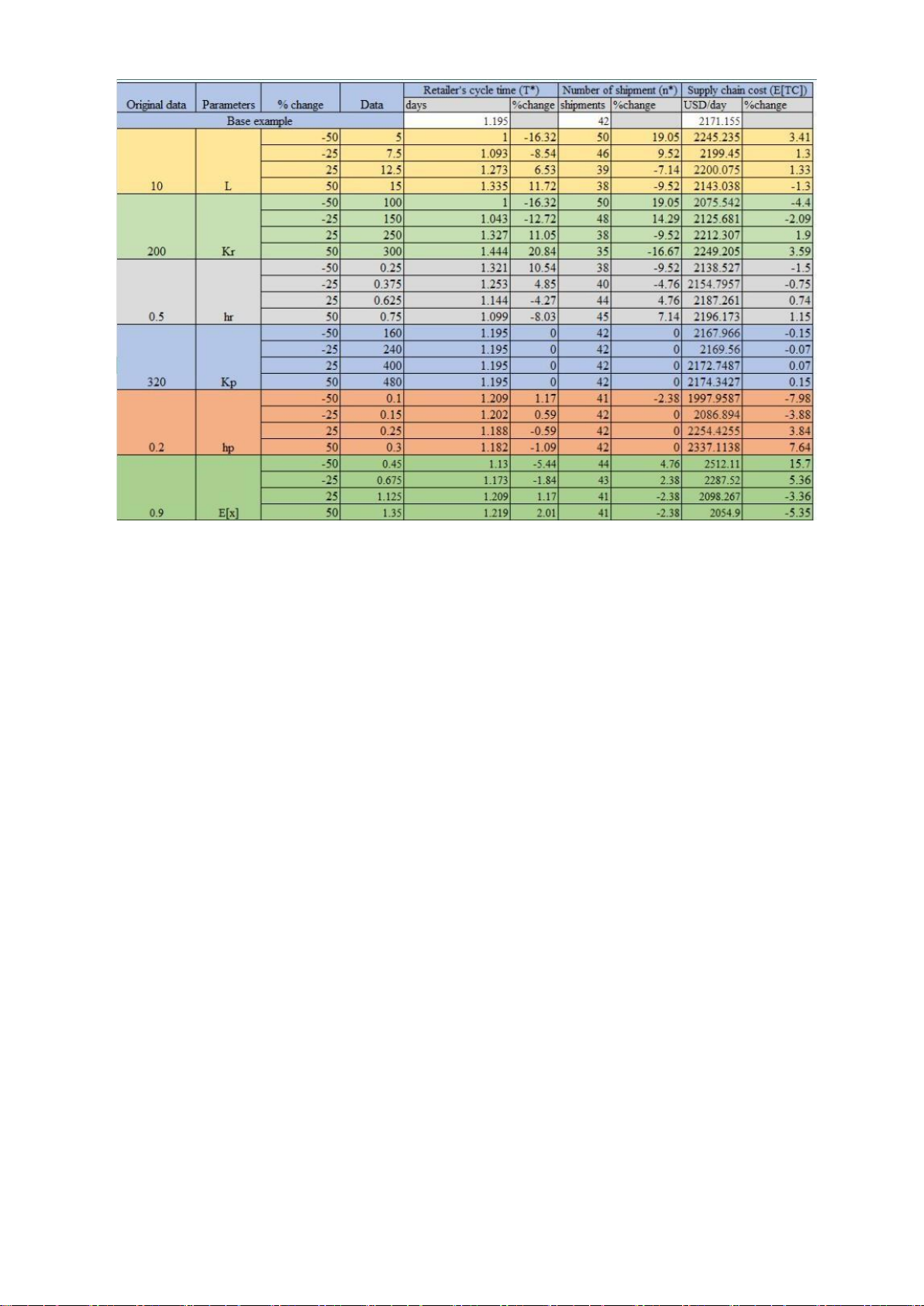
Table 3.2 Sensitivity analysis .................................................................................... 14
Table 4.1 The differences between the assigned paper and this report ..................... 16 LIST OF FIGURES
Figure 1.1 Multi-echelon system is considered ......................................................... 4
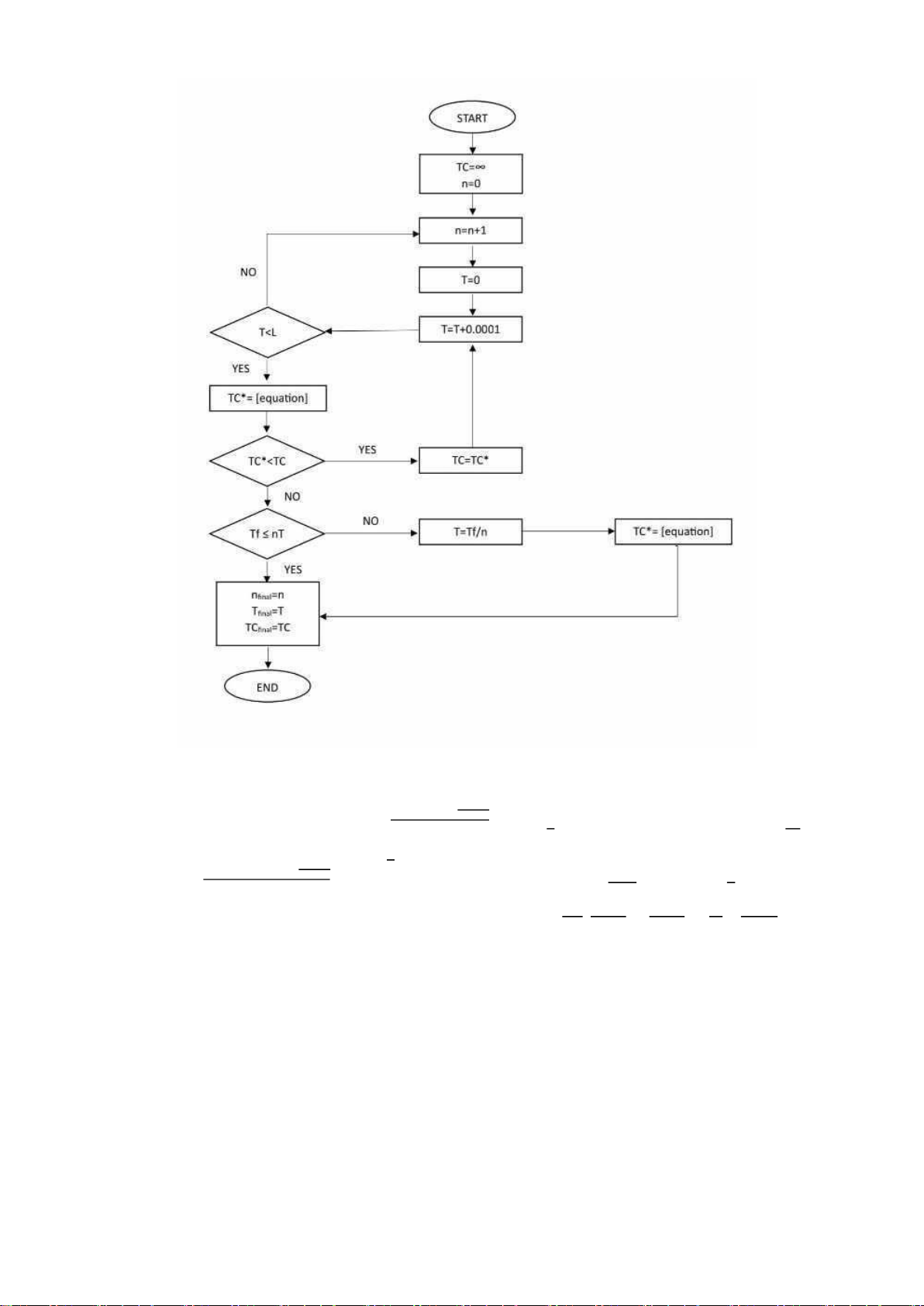
Figure 2.3 Genetic Algorithm Development ............................................................. 7
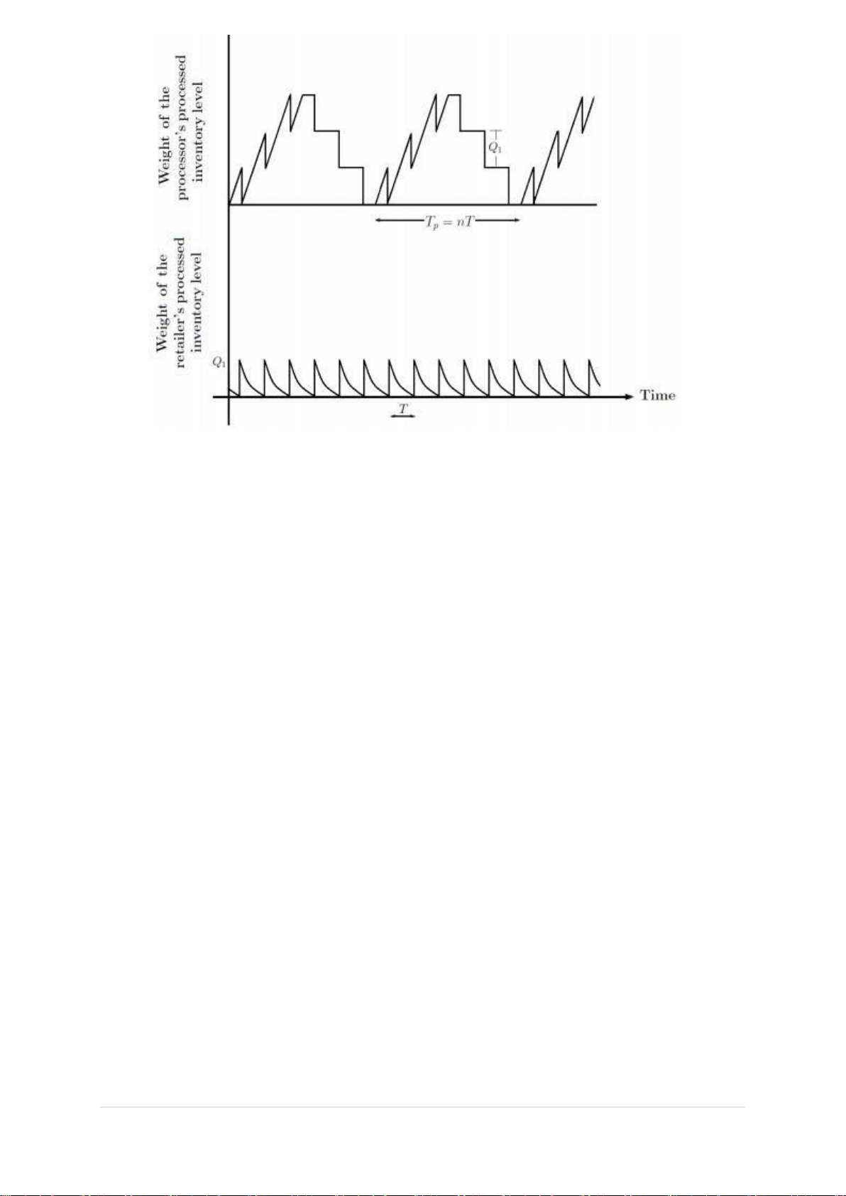
Figure 4.2 The weight of the processed inventory level at the processor and retailer 17 1 | P a g e lOMoARcPSD|47207367
CHAPTER 1 INTRODUCTION 1.1 System description
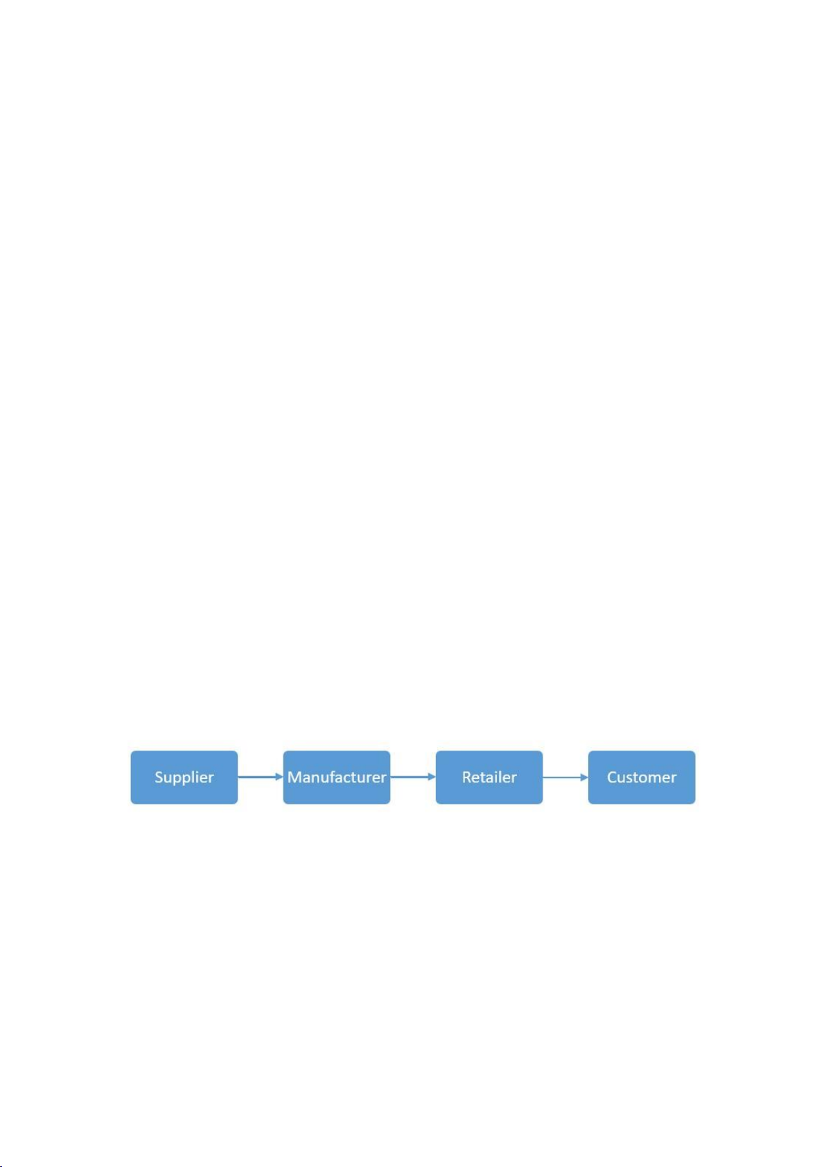
The system that this report applies is multi-echelon system, meaning this system will
take into consideration all inventory levels at each node. The system in this study will
consist of one supplier, one manufacturer, and one retailer.
Figure 1.1 Multi-echelon system is considered
With a multi-echelon fresh product inventory system, customer demand will start the
order from the retailer to the manufacturer, and the manufacturer based on the data
directly from manufacturer will start sending orders to a supplier. To avoid large
capacity and long inventory holding time of fresh goods at each level, the company will
need to design an inventory system to minimize inventory costs for the entire supply chain. 1.2 Problem statement
As customer demand for fresh food increases, factors such as deterioration (expiration
date) and fragility of fresh products become extremely important but at the same time
difficult to control in quantity and quality at each inventory level of the supply chain.
Furthermore, minimizing inventory costs for the entire supply chain is extremely
difficult to deal with. Numerous enterprises face the problem of high inventory to keep
fresh products but need help to control the expiration date of biodegradable goods with
high holding costs. If keeping the stock level low will result in a high risk of lost sales.
Thus, it is necessary to develop a system that controls the amount of inventory at each
level, by reducing inventory costs of the entire supply chain since then the company will
know how many orders to place, how many units each order has, and when to place that
order so that product quality is best and costs are minimized when each echelon is linked together.
1.3 Scope and Limitations 1.3.1 Scope
Our team looks at a case study including a manufacturer selection issue and profit
maximization in this investigation. It is believed that this network consists of a single
product that the manufacturers deliver to the demand within period t. In addition, we
need to determine the best order quantity in the network of one supplier. For a variety
of costs, including demand, farmer setup cost each cycle, and farmer feeding cost per
weight unit per unit time, we generate arbitrary demand data.
1.3.2 Limitation
The most urgent issue is computational complexity, particularly when it comes to
strategies for handling instability in certain circumstances. It may be essential to build
an agent but not an excessive number of scenarios if there is identifiable proof of the
appropriate underlying causes of such instability (such as economic events).
Furthermore, the scenario under examination presents a problem due to no mention of
transportation cost, discount policies, and no shortage that must be made within each
period and the variable demand for items, which impacts the appropriateness of the storage capacity. 3 | P a g e lOMoARcPSD|47207367 CHAPTER 2 METHODOLOGY
2.1 Problem Description
This case study considers the three-echelon inventory system of perishable products
having deterioration rates. The three-echelon inventory system consists of one supplier
at the first level at which the products are fed until they reach the specific weight; one
manufacturer at the second level where products are processed and packaged before
being delivered to other places; and one retailer at the third level, at which the products
are displayed to sell for customers.
The highlight of this work lies in the dependence of the three levels upon each other,
which means the order quantity of manufacturer to the supplier depends on the number
of products that retailer order from manufacturer. Similar to the cycle time of each
echelon, the supplier’s and manufacturer’s cycle times depend upon the retailer’s. The
idea that independent decisions should be avoided even though the decrease in cost for
one node can potentially increase the cost for another node due to the coordination in a
supply chain is also expressed in Zhang et al. (2021), but this paper used a genetic
algorithm to proved the optimization Centralized Strategy has over the Decentralized
Strategy without no details in how to come up with such results. The work in our report
proposes a detailed approach showing the dependence through a specific genetic algorithm.
The aim of this problem is based on the given data to find out the optimal number of
loads n that should be delivered to a retailer at one time, or in other words, to determine
the Economic Order Quantity (EOQ) that Processor should order from Supplier to fulfill
the demand of Retailer, and the retailer’s cycle time T should be to minimize the total
cost of this inventory system.
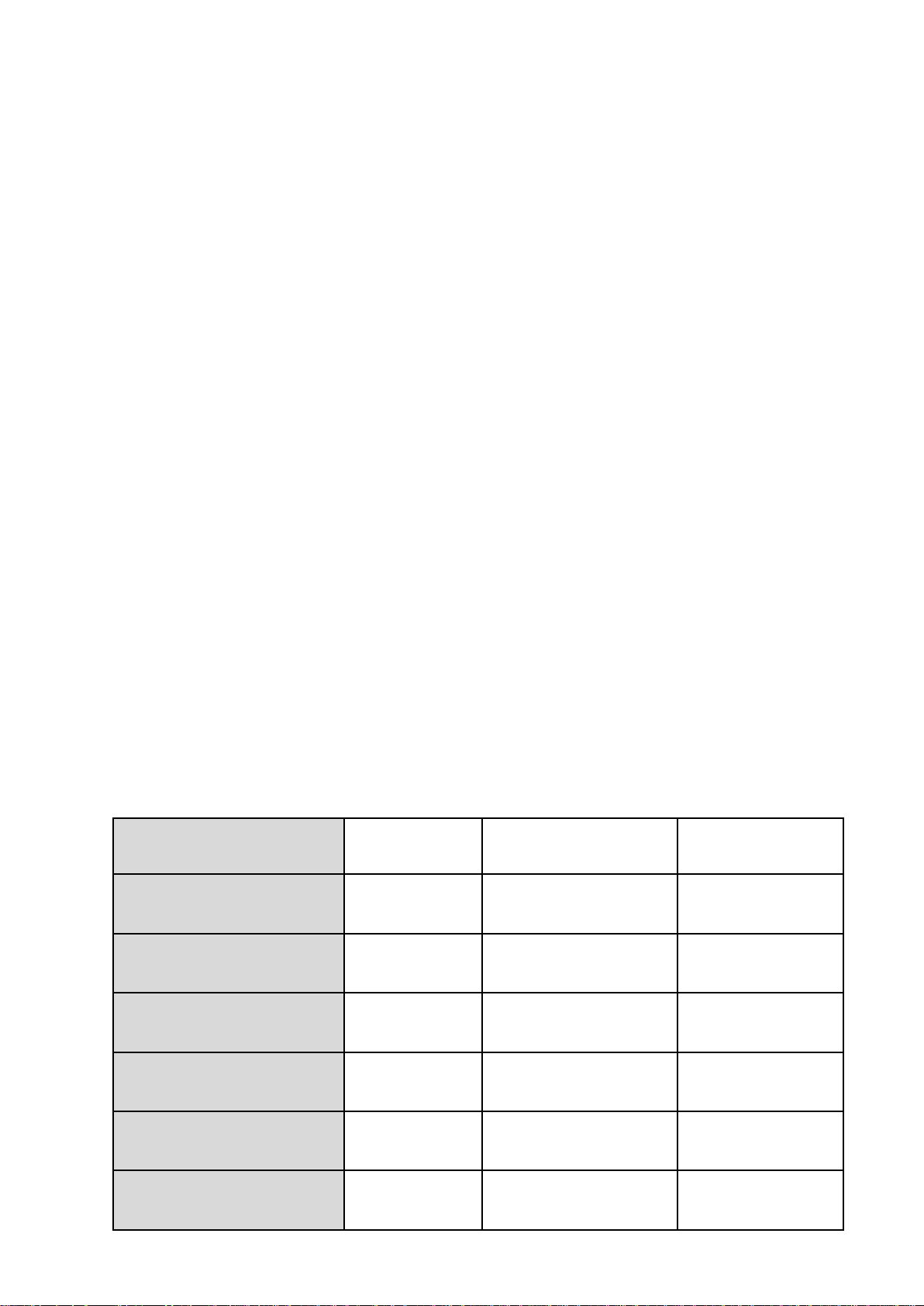
The necessary data for solving this case is given in the table below:
RETAILER MANUFACTURER SUPPLIER Demand (kg) 200 w0 0.5 0.5 0.5 w1 3 3 3 P 300 Kf ($) 400 cf ($/kg/day) 0.5 mf ($/kg/day) 0.1 Kp ($) 320 hp ($/kg/day) 0.2 L (days) 10 10 10 Kr ($) 200 hr ($/kg/day) 0.5 α 6.52 6.52 6.52 β 100 100 100 𝝺 (w1/w0/70 days) 0.09
Table 2.1 Necessary data for solving case study 2.2 Model assumptions:
- Dealing with a three-echelon supply chain model: 1 vendor - 1 processor - 1 retailer.
- Dealing with a single type of perishable product.
- The processing rate is greater than the demand rate.
- Deterioration is taken into consideration under the form of the expiration date of the finished product.
- Beyond the expiration date, the utility of products is over.
- The next shipment from processor to retailer is conducted once the previous shipment is depleted. 5 | P a g e lOMoARcPSD|47207367
2.3 Genetic Algorithm Development
Figure 2.3 Genetic Algorithm Development 1+𝐿
** [equation]= 𝑐𝑓𝑥𝐷(1+𝐿)𝑙𝑛1+𝐿−𝑇 {𝛼𝑇𝑓 + 𝛼 [𝑙𝑛(1 + 𝛽𝑒−𝜆𝑇𝑓) − 𝑙𝑛(1 + 𝛽)]} + 𝐾𝑓 + 𝑇𝑥(𝑤1) 𝜆 𝑛𝑇 1+𝐿
𝑚𝑓(1−𝑥)𝐷(1+𝐿)𝑙𝑛1+𝐿−𝑇 {αTf + 𝛼 −𝜆𝑇𝑓) − 𝑙𝑛(1 + 𝛽]} + ℎ𝑝𝑇𝐷 [(𝑛 − 1)(1 − 𝐷)+𝐷] + 𝐾𝑝 + [𝑙𝑛(1 + 𝛽𝑒 𝑇𝑥(𝑤1) 𝜆 2 𝑃 𝑃 𝑛𝑇 ℎ𝑟𝐷 (1+𝐿)2 1+𝐿 𝑇2 (1+𝐿)𝑇 𝐾𝑟 [ 𝑙𝑛( ) + − ] + 𝑇 2 1+𝐿−𝑇 4 2 𝑇
2.4 Preparation
2.4.1 Parameters W1 Weight of maturity item
x Fraction of the live items that survive throughout the growth period. This factor
determines that x*100 % of the initially ordered items will survive after the growth period ends
D Demand rate for processed items from processor to retailer in weight units per unit time
P Processing rate in weight units per unit time Kf
Farmer’s setup cost per cycle cf Farmer’s feeding cost
per weight unit per unit time Tf Duration of the farmer’s
growth period mf Farmer’s mortality cost per weight
unit per unit time Kp Processor’s setup cost per cycle hp
Processor’s holding cost per weight unit per unit time
L The maximum lifetime (i.e. expiration date) of the processed inventory
Kr Retailer’s ordering cost per cycle hr Retailer’s holding cost per
weight unit per unit time α The items’ asymptotic weight β Constant
of integration λ Growth rate (exponential) of the items
2.4.2 Decision Variables
n Number of shipments from the processor to the retailer per unit cycle of the processor T Retailer’s cycle time
2.4.3 Constraints (1) Tf - n*T ≤ 0
(2) n is an integer: the number of shipments from the processors to the retailers per processing setup (n).
(3) P > D : The demand rate of a retailer should be less than the processing rate to
ensure enough quantity being shipped to the retailer.
(4) L > T : The retailer’s replenishment cycle, T, cannot exceed the expiration date of the processed inventory. 2.5 Objective function
2.5.1 Formulation
The 1st supply chain echelon: Vendor 7 | P a g e lOMoARcPSD|47207367 (i) Feeding Cost: 1+𝐿
FCf = 𝑐𝑓𝑥𝐷(1+𝐿)𝑙𝑛 𝛼
−𝜆𝑇𝑓) − 𝑙𝑛(1 + 𝛽)]}
1+𝐿−𝑇 {𝛼𝑇𝑓 + [𝑙𝑛(1 + 𝛽𝑒 𝑇𝑥(𝑤1) 𝜆 (ii) Set up Cost: 𝐾𝑓 KCf = 𝑛𝑇 (iii) Mortality Cost: 1+𝐿
𝑚𝑓(1−𝑥)𝐷(1+𝐿)𝑙𝑛 𝛼
−𝜆𝑇𝑓) − 𝑙𝑛(1 + 𝛽]} MCf =
1+𝐿−𝑇 {αTf + [𝑙𝑛(1 + 𝛽𝑒 𝑇𝑥(𝑤1) 𝜆
→Total Cost vendor = (i) + (ii) + (iii) 1+𝐿 𝛼
𝑐𝑓𝑥𝐷(1+𝐿)𝑙𝑛
−𝜆𝑇𝑓) − 𝑙𝑛(1 + 𝛽)]} + 𝐾𝑓 + =
1+𝐿−𝑇 {𝛼𝑇𝑓 + [𝑙𝑛(1 + 𝛽𝑒 𝑇𝑥(𝑤1) 𝜆 𝑛𝑇 1+𝐿
𝑚𝑓(1−𝑥)𝐷(1+𝐿)𝑙𝑛1+𝐿−𝑇 {αTf + 𝛼
−𝜆𝑇𝑓) − 𝑙𝑛(1 + 𝛽]} (I) [𝑙𝑛(1 + 𝛽𝑒 𝑇𝑥(𝑤1) 𝜆
The 2nd echelon supply chain: Processor (i) Holding Cost: ℎ𝑝𝑇𝐷 𝐷 𝐷 HCp = [(𝑛 − 1)(1 − )+ ] 2 𝑃 𝑃 (ii) Set up Cost: 𝐾𝑝 KCp = 𝑛𝑇
→Total Cost processor = (i) + (ii) ℎ𝑝𝑇𝐷 𝐷 𝐷 𝐾𝑝 = [(𝑛 − 1)(1 − )+ ]+ (II) 2 𝑃 𝑃 𝑛𝑇
The 3rd echelon supply chain: Retailer (i) Holding Cost: ℎ𝑟𝐷 (1+𝐿)2 1+𝐿 𝑇2 (1+𝐿)𝑇 HCr = [ 𝑙𝑛( ) + − ] 𝑇 2 1+𝐿−𝑇 4 2 (ii) Set up Cost: KCr = 𝐾𝑟 𝑇
→Total Cost retailer = (i) + (ii) ℎ𝑟𝐷 (1+𝐿)2 1+𝐿 𝑇2 (1+𝐿)𝑇 𝐾𝑟 = [𝑙𝑛( ) + − ] + (III) 𝑇 2 1+𝐿−𝑇 4 2 𝑇
2.5.2 Objective function Min z = (I) + (II) + (III) 1+𝐿
= 𝑐𝑓𝑥𝐷(1+𝐿)𝑙𝑛1+𝐿−𝑇 {𝛼𝑇𝑓 + 𝛼 −𝜆𝑇𝑓) − 𝑙𝑛(1 + 𝛽)]} + 𝐾𝑓 + [𝑙𝑛(1 + 𝛽𝑒 𝑇𝑥(𝑤1) 𝜆 𝑛𝑇 1+𝐿
𝑚𝑓(1−𝑥)𝐷(1+𝐿)𝑙𝑛1+𝐿−𝑇 {αTf + 𝛼 [𝑙𝑛(1 + 𝛽𝑒−𝜆𝑇𝑓) − 𝑙𝑛(1 + 𝛽]} + ℎ𝑝𝑇𝐷
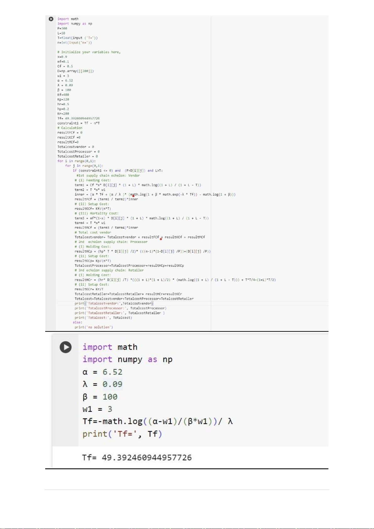
[(𝑛 − 1)(1 − 𝐷 )+𝐷] 𝑇𝑥(𝑤1) 𝜆 2 𝑃 𝑃 𝐾𝑝 ℎ𝑟𝐷 (1+𝐿)2 1+𝐿 𝑇2 (1+𝐿)𝑇 𝐾𝑟 + + [ 𝑙𝑛( ) + − ] + 𝑛𝑇 𝑇 2 1+𝐿−𝑇 4 2 𝑇 2.6 Algorithm STEP 1 import math import numpy as np α = 6.52 λ = 0.09 β = 100 w1 = 3
Tf=-math.log((α-w1)/(β*w1))/ λ print(’Tf=’, Tf) STEP 2 import math import numpy as np P=300 L=10 T=float(input (’T=’)) n=int(input(’n=’)) # Initialize variables x=0.9 mf=0.1 9 | P a g e lOMoARcPSD|47207367 Cf = 0.5 D=np.array([[200]]) w1 = 3 α = 6.52 λ = 0.09 β = 100 Kf=400 Kp=320 hr=0.5 hp=0.2 Kr=60
Tf= 49.392460944957726 constraint1 = Tf - n*T # Calculation resultFCf = 0 resultKCf =0 resultMCf=0 TotalcostVendor = 0
TotalcostProcessor = 0 TotalcostRetailer = 0 for i in range(0,1):
for j in range(0,1): if (constraint1 <= 0) and (P>D[i][j]) and
L>T: #1st supply chain echelon: Vendor # (i) Feeding
Cost: term1 = Cf *x* D[i][j] * (1 + L) * math.log((1 + L) / (1 + L - T)) term2 = T *x* w1
inner = (α * Tf + (α / λ )* (math.log(1 + β * math.exp(-λ * Tf)) - math.log(1 + β)))
resultFCf = (term1 / term2)*inner # (ii) Setup Cost: resultKCf= Kf/(n*T) # (iii) Mortality Cost:
term3 = mf*(1-x) * D[i][j] * (1 + L) * math.log((1 + L) / (1 + L - T)) term4 = T *x* w1
resultMCf = (term3 / term4)*inner # Total cost vendor
TotalcostVendor= TotalcostVendor + resultFCf + resultKCf + resultMCf
# 2nd echelon supply chain: Processor # (i) Holding Cost:
resultHCp = (hp* T * D[i][j] /2)* (((n-1)*(1-D[i][j] /P))+(D[i][j] /P)) # (ii) Setup Cost: resultKCp= Kp/(n*T)
TotalcostProcessor=TotalcostProcessor+resultHCp+resultKCp
# 3rd echelon supply chain: Retailer # (i) Holding Cost:
resultHCr = (hr* D[i][j] /T) *(((1 + L)*(1 + L)/2) * (math.log((1 + L) / (1 + L - T))) + T*T/4-(1+L)*T/2) # (ii) Setup Cost: resultKCr= Kr/T
TotalcostRetailer=TotalcostRetailer+ resultHCr+resultKCr
Totalcost=TotalcostVendor+TotalcostProcessor+TotalcostRetailer
print(’TotalcostVendor:’, Totalcostvendor)
print(’TotalcostProcessor:’, TotalcostProcessor)
print(’TotalcostRetailer:’, TotalcostRetailer )
print(’Totalcost:’, Totalcost) else: print(’no solution’) CHAPTER 3 RESULT
3.1 Result presentation
3.1.1 Result of Decision variables and Objective function
The results obtained are the optimal quantity of shipments delivered from the processor
to the retailer per unit processor cycle time and the retailer’s cycle time. + T = 1.195 + n = 42
Here, the minimized total cost is also calculated:
+ The minimized total cost of supplier is $1,592.7415457665797
+ The minimized total cost of processor is $348.94243873281533
+ The minimized total cost of retailer is $229.47083226599898
+ The minimized total cost of a system is $2,171.154816765394
3.1.2 Result Analysis
From the result, inventory replenishment and shipment strategies are calculated and summarized as follows:
(1) An order of (ny) 3935.244 live newborn items should be placed to fulfill the demand of a retailer.
(2) The total weight of the shipments delivered from the supplier to the processor in
the weight unit is (nQ1) 10,625.1589 kg.
(3) During the whole of a single processor’s cycle, n= 42 shipments to the retailer
within each shipment weights 𝑄1 = 𝐷(1 + 𝐿)ln(
1+1+𝐿−𝑇𝐿 ) = 252.98 kg
(4) The safe interval of time for inventory replenishment is T= 1.195 days to avoid
surplus damaged inventory due to reaching the expiration date.
(5) The new cycle for growing and processing should be conducted every nT= 50.19 days.
(6) Finally, the total inventory cost is minimized to $2,171.1548/day within the
retailer cycle time, T=1.195 days, and n=42 shipments. 11 | P a g e lOMoARcPSD|47207367
3.2 Sensitivity Analysis
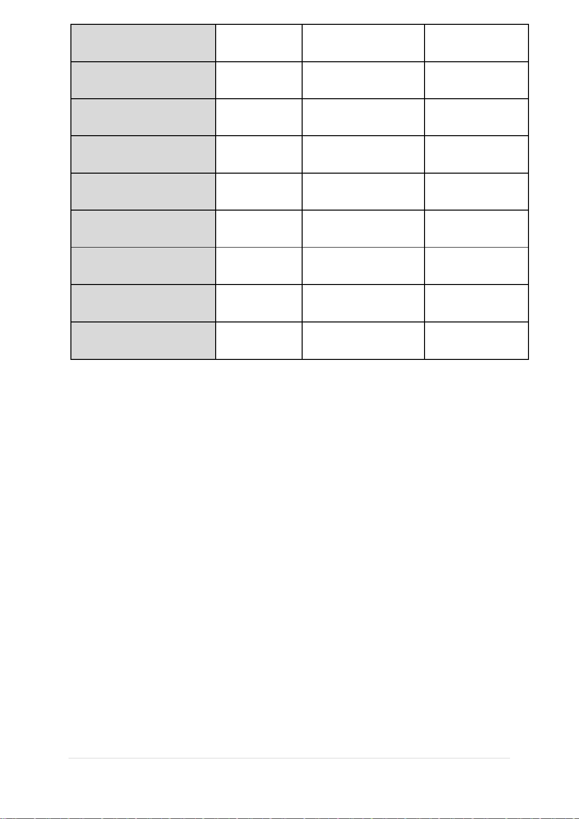
Table 3.2 Sensitivity analysis result
To see how adjustments (increases and decreases of 25% and 50%) to the key input
parameters in the base example affected the objective function (E[TCsc]) and the two
decision variables (T and n), a sensitivity analysis was conducted on those parameters
using Excel Solver. The findings are displayed in the above table, and it is important to
notice the following observations:
For the shelf life (or expiration date) of the processed items affecting the cost of the
supply chain when a 50% loss in shelf life resulted in a roughly 3.5% rise in cost, a
roughly 19% increase in shipments, and about 17% reduction in the retailer's cycle time.
Since the store does not wish to keep the products past their expiration dates. Thus, the
model's optimal solution suggests ordering for relatively smaller lot sizes more
frequently as the product's shelf life is shortened.
Modifications to the retailer's ordering cost when rising order costs is to allow the
retailer to place fewer orders. However, because of the higher holding expenses brought
on by the bigger lot size, this can have a negative impact on the overall cost. For instance,
a 50% increase in ordering costs results in a 20% increase in cycle time. This raises the overall cost by about 4%.
The model's optimal solution reacts to an increase in the retailer's holding costs by
suggesting the retailer order more shipments with smaller lot sizes. The primary
advantage of ordering smaller lot sizes is that they have relatively lower holding costs.
This is because smaller lots require fewer items to be stored, and smaller lots also result
in a shorter cycle time for the retailer, which lowers the amount of time the processed
inventory is stored and, ultimately, the holding costs. For instance, a 50% rise in the
retailer's holding costs led to an 8% decrease in cycle time and a 7% increase in shipments.
Modifications to the processor's setup indicate that the ideal number of cycle times and
shipments to the merchant will not alter, even if the processor's setup costs drop. This
demonstrates that altering the setup cost of the processor has little effect on the overall cost.
The model's optimal solution reacts to a rise in the processor's holding costs by
shortening the cycle time. This shortens the amount of time the processed inventory is
stored, which lowers the holding costs. For instance, a 50% increase in holding costs
results in a 1% reduction in cycle time and raises the overall cost by about 7.7%.
When the fraction of live things that survive during the growing cycle rises, the number
of shipments and the overall cost drop as the cycle time grows. The best solution of the
model reacts in this way because the enhanced survival rate allows a smaller lot size of
newborn items to meet the given demand rate for processed goods. Because there are a
smaller number of shipments to the retailer, this lowers the overall supply chain cost. CHAPTER 4 DISCUSSION
4.1 Comparison of assigned paper and our work (1) Similarities:
Both of them consider the three-echelon system and enhance the inventory management
of a multi-echelon supply chain of perishable products. The outcome of them is to
minimize the total inventory cost of the system. (2) Differences: ASSIGNED PAPER THIS REPORT In consideration Non Transportation cost and reorder point 13 | P a g e lOMoARcPSD|47207367 Output Compare decentralized strategy and centralized Mainly determine the strategy and end up stock cycle of the retailer
concluding the centralized (3rd level) to give insight one result in the optimal regarding how long the inventory management perishable product should be kept in the final level of a multi-echelon supply chain to avoid potential inventory risks (overstock, etc.) No Yes Genetic Algorithm Proposal
Table 4.1 The differences between the assigned paper and this report
4.2. Why the formulation of the paper assigned is not used in this matter?
The assigned paper solved the problem, minimizing the total inventory cost. In the
context of lacking the impact that echelons have on each other, our work is based on the
research of considering this effect and giving the idea of making the order quantity
decisions jointly with the members in a supply chain.
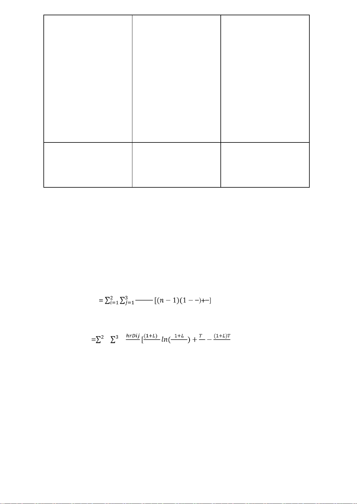
This point can be verified through the difference in the Holding Cost Formula between the processor and retailer: ℎ𝑝𝑇𝐷𝑖𝑗 𝐷 𝐷 + Processor: HCp 2 𝑃 𝑃 2 2 + Retailer: HCr i=1 𝑗=1 𝑇 2 1+𝐿−𝑇 4 2 ]
These two formulas are formulated based on the characteristics of a multi-echelon
supply chain, are multiplications of the areas under the graphs, which show the impact
supply chain levels have on each other, and the time interval T.
Figure 4.2 The weight of the processed inventory level at the processor and the retailer
Whereas the assigned paper uses the same Holding Cost formula for every node in every
level of the multi-echelon model when applying Decentralized strategy, and no detailed
approach was mentioned for Centralized strategy.
4.3 Limitation
(1) The used data was collected based on Sebatjane et al. (2022) paper since we lack
deep knowledge about the deterioration and relevant factors, namely the growth
rate, fraction of the live items, constant of integration, and the items’ asymptotic
weight. More understanding and scientific applied data will result in more applicability of the model.
(2) The simplification of the model in the number of nodes in each echelon
(3) Lack of comparison with the assigned paper regarding its methodology to clarify
that our optimal results have the same effectiveness due to the difference in the
type of multi-echelon model (1-1-1 and 1-2-3) and the difference in genetic algorithm. CHAPTER 5 CONCLUSION
Delivery of perishable products from supplier to customer is always one of the most
difficult issues currently. The managers need to think of how to control the deterioration
rate of this kind of product, how to reduce the number of damaged items during a long 15 | P a g e lOMoARcPSD|47207367
delivery time, and how to optimize the cycle time when transferring them. They must
decide the appropriate policies to satisfy conditions and solve those problems.
This research is carried out to determine the optimal solution for perishable products in
a multi-echelon system. By involving deterioration rate in formulas, it could calculate
and give a more accurate result that helps to achieve the more optimal policy for the
whole system. Specifically, the research considers the three-echelon system which
includes one supplier, one manufacturer, and one retailer. The objective is to show the
optimal number of shipments from manufacturer to retailer in a unit cycle time of the
processor and the retailer’s cycle time so that the inventory cost of this system is minimized.
Although there are some limitations to computational complexity, assuming no mention
of transportation cost, discount policies, or no shortage, it could be a premise for other
research later so that people can reach nearer to the most optimal solution. REFERENCES [1]
Sebatjane, M., Adetunji, O. (2022) Optimal inventory replenishment and
shipment policies in a three-echelon supply chain for growing items with expiration
dates. OPSEARCH 59, 809–838 (2022). https://doi.org/10.1007/s12597-022-00572-6 [2]
Zhang, Y., Chai, Y., & Ma, L. (2021). Research on Multi-Echelon Inventory
Optimization for Fresh Products in Supply Chains. Sustainability, 13(11), 6309.
https://doi.org/10.3390/su13116309 APPENDIX 1. Python code
The results were obtained using Python software 17 | P a g e lOMoARcPSD|47207367
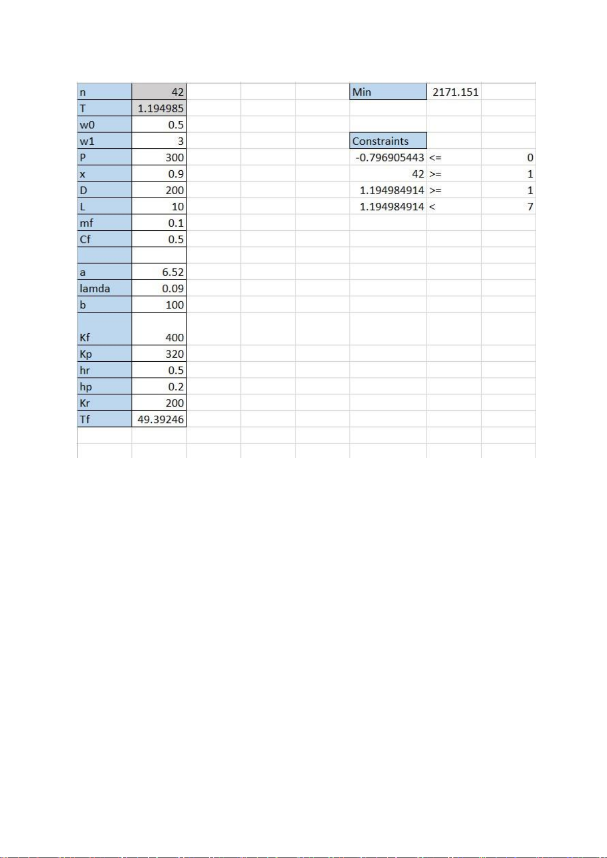
2. Sensitivity Analysis
The results are obtained using Excel Solver.