Ôn tập cuối kỳ: Logistic Regression môn Học máy | Trường Đại học Công nghệ, Đại học Quốc gia Hà Nội
Ôn tập cuối kỳ: Logistic Regression môn Học máy | Trường Đại học Công nghệ, Đại học Quốc gia Hà Nội. Tài liệu được sưu tầm giúp bạn tham khảo, ôn tập và đạt kết quả cao. Mời bạn đọc đón xem.
Môn: Học máy 10 tài liệu
Trường: Trường Đại học Công nghệ, Đại học Quốc gia Hà Nội 824 tài liệu
Tác giả:


Preview text:
Logistic Regression
In this exercise, you will implement logistic regression and apply it to two different datasets. Outline • 1 - Packages • 2 - Logistic Regression – 2.1 Problem Statement –
2.2 Loading and visualizing the data – 2.3 Sigmoid function –
2.4 Cost function for logistic regression –
2.5 Gradient for logistic regression –
2.6 Learning parameters using gradient descent –
2.7 Plotting the decision boundary –
2.8 Evaluating logistic regression •
3 - Regularized Logistic Regression – 3.1 Problem Statement –
3.2 Loading and visualizing the data – 3.3 Feature mapping –
3.4 Cost function for regularized logistic regression –
3.5 Gradient for regularized logistic regression –
3.6 Learning parameters using gradient descent –
3.7 Plotting the decision boundary –
3.8 Evaluating regularized logistic regression model •
You run all code, explain the code and results, answer questions, capture picture and input into your report 1 - Packages
First, let's run the cell below to import all the packages that you will need during this assignment. •
numpy is the fundamental package for scientific computing with Python. •
matplotlib is a famous library to plot graphs in Python. •
utils.py contains helper functions for this assignment. You do not need to modify code in this file. import numpy as np
import matplotlib.pyplot as plt from utils import * import copy import math %matplotlib inline 2 - Logistic Regression
In this part of the exercise, you will build a logistic regression model to predict whether a
student gets admitted into a university. 2.1 Problem Statement
Suppose that you are the administrator of a university department and you want to determine
each applicant’s chance of admission based on their results on two exams. •
You have historical data from previous applicants that you can use as a training set for logistic regression. •
For each training example, you have the applicant’s scores on two exams and the admissions decision. •
Your task is to build a classification model that estimates an applicant’s probability of
admission based on the scores from those two exams.
2.2 Loading and visualizing the data
You will start by loading the dataset for this task. •
The load_dataset() function shown below loads the data into variables X_train and y_train –
X_train contains exam scores on two exams for a student –
y_train is the admission decision •
y_train = 1 if the student was admitted •
y_train = 0 if the student was not admitted –
Both X_train and y_train are numpy arrays. # load dataset
X_train, y_train = load_data("data/ex2data1.txt") View the variables
Let's get more familiar with your dataset. •
A good place to start is to just print out each variable and see what it contains.
The code below prints the first five values of X_train and the type of the variable.
print("First five elements in X_train are:\n", X_train[:5])
print("Type of X_train:",type(X_train))
Now print the first five values of y_train
print("First five elements in y_train are:\n", y_train[:5])
print("Type of y_train:",type(y_train))
Check the dimensions of your variables
Another useful way to get familiar with your data is to view its dimensions. Let's print the shape
of X_train and y_train and see how many training examples we have in our dataset.
print ('The shape of X_train is: ' + str(X_train.shape))
print ('The shape of y_train is: ' + str(y_train.shape))
print ('We have m = %d training examples' % (len(y_train))) Visualize your data
Before starting to implement any learning algorithm, it is always good to visualize the data if possible. •
The code below displays the data on a 2D plot (as shown below), where the axes are the
two exam scores, and the positive and negative examples are shown with different markers. •
We use a helper function in the utils.py file to generate this plot. # Plot examples
plot_data(X_train, y_train[:], pos_label="Admitted", neg_label="Not admitted") # Set the y-axis label
plt.ylabel('Exam 2 score') # Set the x-axis label
plt.xlabel('Exam 1 score') plt.legend(loc="upper right") plt.show()
Your goal is to build a logistic regression model to fit this data. •
With this model, you can then predict if a new student will be admitted based on their scores on the two exams. 2.3 Sigmoid function
Recall that for logistic regression, the model is represented as f
( x)=g(w ⋅ x+b) w ,b
where function g is the sigmoid function. The sigmoid function is defined as: g ( z)= 1 1+e−z
Let's implement the sigmoid function first, so it can be used by the rest of this assignment. Exercise 1
Please complete the sigmoid function to calculate g ( z)= 1 1+e−z Note that •
z is not always a single number, but can also be an array of numbers. •
If the input is an array of numbers, we'd like to apply the sigmoid function to each value in the input array.
If you get stuck, you can check out the hints presented after the cell below to help you with the implementation. # UNQ_C1 # GRADED FUNCTION: sigmoid def sigmoid(z): """ Compute the sigmoid of z Args:
z (ndarray): A scalar, numpy array of any size. Returns:
g (ndarray): sigmoid(z), with the same shape as z """
### START CODE HERE ### g = 1/(1+np.exp(-z))
### END SOLUTION ### return g Click for hints
numpy has a function called np.exp(), which offers a convinient way to calculate the
exponential ( ez) of all elements in the input array (z).
When you are finished, try testing a few values by calling sigmoid(x) in the cell below. •
For large positive values of x, the sigmoid should be close to 1, while for large negative
values, the sigmoid should be close to 0. •
Evaluating sigmoid(0) should give you exactly 0.5.
print ("sigmoid(0) = " + str(sigmoid(0)))
Expected Output: sigmoid(0) 0.5 •
As mentioned before, your code should also work with vectors and matrices. For a
matrix, your function should perform the sigmoid function on every element.
print ("sigmoid([ -1, 0, 1, 2]) = " + str(sigmoid(np.array([-1, 0, 1, 2])))) # UNIT TESTS from public_tests import * sigmoid_test(sigmoid)
Expected Output: sigmoid([-1, 0, 1, 2]) [0.26894142 0.5 0.73105858 0.88079708]
2.4 Cost function for logistic regression
In this section, you will implement the cost function for logistic regression. Exercise 2
Please complete the compute_cost function using the equations below.
Recall that for logistic regression, the cost function is of the form m −1
J (w , b )= 1 ∑ [l o s s(f (x(i)), y(i)) m w ,b i=0 where •
m is the number of training examples in the dataset •
l o s s(f (x(i)), y(i)) is the cost for a single data point, which is - w ,b
l o s s (f (x(i)), y(i))=¿ w ,b • f
(x(i)) is the model's prediction, while y(i), which is the actual label w ,b • f
(x(i))=g(w ⋅ x(i)+b) where function g is the sigmoid function. w ,b –
It might be helpful to first calculate an intermediate variable z
(x(i))=w ⋅ x(i)+b=w x(i)+...+w x(i) +b where n is the number of features, w ,b 0 0 n −1 n− 1 before calculating f
(x(i))=g(z (x(i)) w ,b w , b Note: •
As you are doing this, remember that the variables X_train and y_train are not scalar
values but matrices of shape (m , n) and (𝑚,1) respectively, where 𝑛 is the number of
features and 𝑚 is the number of training examples. •
You can use the sigmoid function that you implemented above for this part.
If you get stuck, you can check out the hints presented after the cell below to help you with the implementation. # UNQ_C2
# GRADED FUNCTION: compute_cost
def compute_cost(X, y, w, b, lambda_= 1): """
Computes the cost over all examples Args:
X : (ndarray Shape (m,n)) data, m examples by n features
y : (array_like Shape (m,)) target value
w : (array_like Shape (n,)) Values of parameters of the model
b : scalar Values of bias parameter of the model lambda_: unused placeholder Returns: total_cost: (scalar) cost """ m, n = X.shape
### START CODE HERE ### cost = 0 for i in range(m): z = np.dot(X[i],w) + b f_wb = sigmoid(z)
cost += -y[i]*np.log(f_wb) - (1-y[i])*np.log(1-f_wb) total_cost = cost/m
### END CODE HERE ### return total_cost
Run the cells below to check your implementation of the compute_cost function with two
different initializations of the parameters w m, n = X_train.shape
# Compute and display cost with w initialized to zeroes initial_w = np.zeros(n) initial_b = 0.
cost = compute_cost(X_train, y_train, initial_w, initial_b)
print('Cost at initial w (zeros): {:.3f}'.format(cost))
Expected Output: Cost at initial w (zeros) 0.693
# Compute and display cost with non-zero w
test_w = np.array([0.2, 0.2]) test_b = -24.
cost = compute_cost(X_train, y_train, test_w, test_b)
print('Cost at test w,b: {:.3f}'.format(cost)) # UNIT TESTS
compute_cost_test(compute_cost)
Expected Output: Cost at test w,b 0.218
2.5 Gradient for logistic regression
In this section, you will implement the gradient for logistic regression.
Recall that the gradient descent algorithm is:
$$\begin{align*}& \text{repeat until convergence:} \; \lbrace \newline \; & b := b - \alpha \frac{\
partial J(\mathbf{w},b)}{\partial b} \newline \; & w_j := w_j - \alpha \frac{\partial J(\
mathbf{w},b)}{\partial w_j} \tag{1} \; & \text{for j := 0..n-1}\newline & \rbrace\end{align*}$$
where, parameters b, w j are all updated simultaniously Exercise 3
∂ J ( w , b) ∂ J ( w , b)
Please complete the compute_gradient function to compute , from ∂ w ∂ b equations (2) and (3) below. ∂ J ( w , b) m −1
= 1 ∑ (f ( x(i))− y(i)) ∂ b m w, b i=0 ∂ J ( w , b) m −1
= 1 ∑ (f ( x(i))− y(i)) x(i) ∂ w m w, b j j i=0 •
m is the number of training examples in the dataset • f
(x(i)) is the model's prediction, while y(i) is the actual label w ,b •
Note: While this gradient looks identical to the linear regression gradient, the
formula is actually different because linear and logistic regression have different definitions of f ( x). w ,b
As before, you can use the sigmoid function that you implemented above and if you get stuck,
you can check out the hints presented after the cell below to help you with the implementation. # UNQ_C3
# GRADED FUNCTION: compute_gradient
def compute_gradient(X, y, w, b, lambda_=None): """
Computes the gradient for logistic regression Args:
X : (ndarray Shape (m,n)) variable such as house size
y : (array_like Shape (m,1)) actual value
w : (array_like Shape (n,1)) values of parameters of the model
b : (scalar) value of parameter of the model lambda_: unused placeholder. Returns
dj_dw: (array_like Shape (n,1)) The gradient of the cost w.r.t. the parameters w.
dj_db: (scalar) The gradient of the cost w.r.t. the parameter b. """ m, n = X.shape dj_dw = np.zeros(w.shape) dj_db = 0.
### START CODE HERE ### for i in range(m):
f_wb_i = sigmoid(np.dot(X[i],w) + b) err_i = f_wb_i - y[i] for j in range(n):
dj_dw[j] = dj_dw[j] + err_i * X[i,j] dj_db = dj_db + err_i dj_dw = dj_dw/m dj_db = dj_db/m
### END CODE HERE ### return dj_db, dj_dw Click for hints •
Here's how you can structure the overall implementation for this function ```python
def compute_gradient(X, y, w, b, lambda_=None): m, n = X.shape dj_dw = np.zeros(w.shape) dj_db = 0. ### START CODE HERE ### for i in range(m):
# Calculate f_wb (exactly as you did in the compute_cost function above) f_wb =
# Calculate the gradient for b from this example
dj_db_i = # Your code here to calculate the error # add that to dj_db dj_db += dj_db_i
# get dj_dw for each attribute for j in range(n):
# You code here to calculate the gradient from the
i-th example for j-th attribute dj_dw_ij = dj_dw[j] += dj_dw_ij
# divide dj_db and dj_dw by total number of examples dj_dw = dj_dw / m dj_db = dj_db / m ### END CODE HERE ### return dj_db, dj_dw ```
If you're still stuck, you can check the hints presented below to figure out how to
calculate f_wb, dj_db_i and dj_dw_ij
Hint to calculate f_wb Recall that you calculated f_wb in compute_cost above
— for detailed hints on how to calculate each intermediate term, check out the hints
section below that exercise More hints to calculate f_wb You can
calculate f_wb as for i in range(m):
# Calculate f_wb (exactly how you did it in the compute_cost function above) z_wb =
0 # Loop over each feature for j in range(n): # Add the corresponding term to z_wb
z_wb_ij = X[i, j] * w[j] z_wb += z_wb_ij # Add bias term z_wb += b
# Calculate the prediction from the model f_wb = sigmoid(z_wb)
Hint to calculate dj_db_i You can calculate dj_db_i as dj_db_i = f_wb - y[i]
Hint to calculate dj_dw_ij You can calculate dj_dw_ij as dj_dw_ij = (f_wb - y[i])* X[i][j]
Run the cells below to check your implementation of the compute_gradient function with
two different initializations of the parameters w
# Compute and display gradient with w initialized to zeroes initial_w = np.zeros(n) initial_b = 0.
dj_db, dj_dw = compute_gradient(X_train, y_train, initial_w, initial_b)
print(f'dj_db at initial w (zeros):{dj_db}' )
print(f'dj_dw at initial w (zeros):{dj_dw.tolist()}' )
Expected Output: dj_db at initial w (zeros) -0.1 ddj_dw at initial w (zeros): [-
12.00921658929115, -11.262842205513591]
# Compute and display cost and gradient with non-zero w
test_w = np.array([ 0.2, -0.5]) test_b = -24
dj_db, dj_dw = compute_gradient(X_train, y_train, test_w, test_b)
print('dj_db at test_w:', dj_db)
print('dj_dw at test_w:', dj_dw.tolist()) # UNIT TESTS
compute_gradient_test(compute_gradient)
Expected Output: dj_db at initial w (zeros) -0.5999999999991071 ddj_dw at initial w (zeros):
[-44.8313536178737957, -44.37384124953978]
2.6 Learning parameters using gradient descent
Similar to the previous assignment, you will now find the optimal parameters of a logistic
regression model by using gradient descent. •
You don't need to implement anything for this part. Simply run the cells below. •
A good way to verify that gradient descent is working correctly is to look at the
value of J (w , b ) and check that it is decreasing with each step. •
Assuming you have implemented the gradient and computed the cost correctly, your
value of J (w , b ) should never increase, and should converge to a steady value by the end of the algorithm.
def gradient_descent(X, y, w_in, b_in, cost_function,
gradient_function, alpha, num_iters, lambda_): """
Performs batch gradient descent to learn theta. Updates theta by taking
num_iters gradient steps with learning rate alpha Args: X : (array_like Shape (m, n) y : (array_like Shape (m,))
w_in : (array_like Shape (n,)) Initial values of parameters of the model
b_in : (scalar) Initial value of parameter of the model
cost_function: function to compute cost alpha : (float) Learning rate
num_iters : (int) number of iterations to run gradient descent
lambda_ (scalar, float) regularization constant Returns:
w : (array_like Shape (n,)) Updated values of parameters of the model after running gradient descent
b : (scalar) Updated value of parameter of the model after running gradient descent """
# number of training examples m = len(X)
# An array to store cost J and w's at each iteration primarily for graphing later J_history = [] w_history = [] for i in range(num_iters):
# Calculate the gradient and update the parameters
dj_db, dj_dw = gradient_function(X, y, w_in, b_in, lambda_)
# Update Parameters using w, b, alpha and gradient
w_in = w_in - alpha * dj_dw b_in = b_in - alpha * dj_db
# Save cost J at each iteration
if i<100000: # prevent resource exhaustion
cost = cost_function(X, y, w_in, b_in, lambda_) J_history.append(cost)
# Print cost every at intervals 10 times or as many iterations if < 10
if i% math.ceil(num_iters/10) == 0 or i == (num_iters-1): w_history.append(w_in)
print(f"Iteration {i:4}: Cost {float(J_history[-1]):8.2f} ")
return w_in, b_in, J_history, w_history #return w and J,w history for graphing
Now let's run the gradient descent algorithm above to learn the parameters for our dataset. Note
The code block below takes a couple of minutes to run, especially with a non-vectorized version.
You can reduce the iterations to test your implementation and iterate faster. If you have
time, try running 100,000 iterations for better results. np.random.seed(1)
initial_w = 0.01 * (np.random.rand(2).reshape(-1,1) - 0.5) initial_b = -8
# Some gradient descent settings iterations = 10000 alpha = 0.001
w,b, J_history,_ = gradient_descent(X_train ,y_train, initial_w, initial_b,
compute_cost, compute_gradient, alpha, iterations, 0) # With the following settings np.random.seed(1)
intial_w = 0.01 * (np.random.rand(2).reshape(-1,1) - 0.5) initial_b = -8 iterations = 10000 alpha = 0.001 # Iteration 0: Cost 1.01 Iteration 1000: Cost 0.31 Iteration 2000: Cost 0.30 Iteration 3000: Cost 0.30 Iteration 4000: Cost 0.30 Iteration 5000: Cost 0.30 Iteration 6000: Cost 0.30 Iteration 7000: Cost 0.30 Iteration 8000: Cost 0.30 Iteration 9000: Cost 0.30 Iteration 9999: Cost 0.30
2.7 Plotting the decision boundary
We will now use the final parameters from gradient descent to plot the linear fit. If you
implemented the previous parts correctly, you should see the following plot:
We will use a helper function in the utils.py file to create this plot.
plot_decision_boundary(w, b, X_train, y_train)
2.8 Evaluating logistic regression
We can evaluate the quality of the parameters we have found by seeing how well the learned
model predicts on our training set.
You will implement the predict function below to do this. Exercise 4
Please complete the predict function to produce 1 or 0 predictions given a dataset and a
learned parameter vector w and b. •
First you need to compute the prediction from the model f (x(i))=g(w ⋅ x(i)) for every example –
You've implemented this before in the parts above •
We interpret the output of the model (f (x(i))) as the probability that y(i)=1 given x(i) and parameterized by w. •
Therefore, to get a final prediction ( y(i)=0 or y(i)=1) from the logistic regression
model, you can use the following heuristic -
if f (x(i))>¿0.5, predict y(i)=1
if f (x(i))<0.5, predict y(i)=0
If you get stuck, you can check out the hints presented after the cell below to help you with the implementation. # UNQ_C4 # GRADED FUNCTION: predict def predict(X, w, b): """
Predict whether the label is 0 or 1 using learned logistic regression parameters w Args: X : (ndarray Shape (m, n))
w : (array_like Shape (n,)) Parameters of the model
b : (scalar, float) Parameter of the model Returns: p: (ndarray (m,1))
The predictions for X using a threshold at 0.5 """
# number of training examples m, n = X.shape p = np.zeros(m)
### START CODE HERE ###
# Loop over each example for i in range(m): z_wb = np.dot(X[i],w) # Loop over each feature for j in range(n):
# Add the corresponding term to z_wb z_wb += 0 # Add bias term z_wb += b
# Calculate the prediction for this example f_wb = sigmoid(z_wb) # Apply the threshold
p[i] = 1 if f_wb>0.5 else 0
### END CODE HERE ### return p
Once you have completed the function predict, let's run the code below to report the training
accuracy of your classifier by computing the percentage of examples it got correct. # Test your predict code np.random.seed(1) tmp_w = np.random.randn(2) tmp_b = 0.3
tmp_X = np.random.randn(4, 2) - 0.5
tmp_p = predict(tmp_X, tmp_w, tmp_b)
print(f'Output of predict: shape {tmp_p.shape}, value {tmp_p}') # UNIT TESTS predict_test(predict) Expected output
Now let's use this to compute the accuracy on the training set
#Compute accuracy on our training set p = predict(X_train, w,b)
print('Train Accuracy: %f'%(np.mean(p == y_train) * 100))
3 - Regularized Logistic Regression
In this part of the exercise, you will implement regularized logistic regression to predict whether
microchips from a fabrication plant passes quality assurance (QA). During QA, each microchip
goes through various tests to ensure it is functioning correctly. 3.1 Problem Statement
Suppose you are the product manager of the factory and you have the test results for some
microchips on two different tests. •
From these two tests, you would like to determine whether the microchips should be accepted or rejected. •
To help you make the decision, you have a dataset of test results on past microchips,
from which you can build a logistic regression model.
3.2 Loading and visualizing the data
Similar to previous parts of this exercise, let's start by loading the dataset for this task and visualizing it. •
The load_dataset() function shown below loads the data into variables X_train and y_train –
X_train contains the test results for the microchips from two tests –
y_train contains the results of the QA •
y_train = 1 if the microchip was accepted •
y_train = 0 if the microchip was rejected –
Both X_train and y_train are numpy arrays. # load dataset
X_train, y_train = load_data("data/ex2data2.txt") View the variables
The code below prints the first five values of X_train and y_train and the type of the variables. # print X_train
print("X_train:", X_train[:5])
print("Type of X_train:",type(X_train)) # print y_train
print("y_train:", y_train[:5])
print("Type of y_train:",type(y_train))
Check the dimensions of your variables
Another useful way to get familiar with your data is to view its dimensions. Let's print the shape
of X_train and y_train and see how many training examples we have in our dataset.
print ('The shape of X_train is: ' + str(X_train.shape))
print ('The shape of y_train is: ' + str(y_train.shape))
print ('We have m = %d training examples' % (len(y_train))) Visualize your data
The helper function plot_data (from utils.py) is used to generate a figure like Figure 3,
where the axes are the two test scores, and the positive (y = 1, accepted) and negative (y = 0,
rejected) examples are shown with different markers. # Plot examples
plot_data(X_train, y_train[:], pos_label="Accepted", neg_label="Rejected") # Set the y-axis label
plt.ylabel('Microchip Test 2') # Set the x-axis label
plt.xlabel('Microchip Test 1') plt.legend(loc="upper right") plt.show()
Figure 3 shows that our dataset cannot be separated into positive and negative examples by a
straight-line through the plot. Therefore, a straight forward application of logistic regression
will not perform well on this dataset since logistic regression will only be able to find a linear decision boundary. 3.3 Feature mapping
One way to fit the data better is to create more features from each data point. In the provided
function map_feature, we will map the features into all polynomial terms of x1 and x2 up to the sixth power. 2 x x 1 2
m a p e a t u r e ( x)= 2 f
[x1x2x1x2)x31⋮x51x2x62
As a result of this mapping, our vector of two features (the scores on two QA tests) has been
transformed into a 27-dimensional vector. •
A logistic regression classifier trained on this higher-dimension feature vector will have a
more complex decision boundary and will be nonlinear when drawn in our 2-dimensional plot. •
We have provided the map_feature function for you in utils.py.
print("Original shape of data:", X_train.shape)
mapped_X = map_feature(X_train[:, 0], X_train[:, 1])
print("Shape after feature mapping:", mapped_X.shape)
Let's also print the first elements of X_train and mapped_X to see the tranformation.
print("X_train[0]:", X_train[0])
print("mapped X_train[0]:", mapped_X[0])
While the feature mapping allows us to build a more expressive classifier, it is also more
susceptible to overfitting. In the next parts of the exercise, you will implement regularized
logistic regression to fit the data and also see for yourself how regularization can help combat the overfitting problem.
3.4 Cost function for regularized logistic regression
In this part, you will implement the cost function for regularized logistic regression.
Recall that for regularized logistic regression, the cost function is of the form m −1 n −1
J (w , b )= 1 ∑ [− y(i)log (f ( x(i)) −(1− y(i)) log(1−f (x(i)) )+ λ ∑ w2 m w , b w ,b j i=0 2 m j=0
Compare this to the cost function without regularization (which you implemented above), which is of the form m− 1
J (w . b )= 1 ∑ ¿¿ m i=0
The difference is the regularization term, which is λ n−1 ∑ w2 2m j j=0
Note that the b parameter is not regularized. Exercise 5
Please complete the compute_cost_reg function below to calculate the following term for each element in w λ n−1 ∑ w2 2m j j=0
The starter code then adds this to the cost without regularization (which you computed above in
compute_cost) to calculate the cost with regulatization.
If you get stuck, you can check out the hints presented after the cell below to help you with the implementation. # UNQ_C5
def compute_cost_reg(X, y, w, b, lambda_ = 1): """
Computes the cost over all examples Args:
X : (array_like Shape (m,n)) data, m examples by n features
y : (array_like Shape (m,)) target value
w : (array_like Shape (n,)) Values of parameters of the model
b : (array_like Shape (n,)) Values of bias parameter of the model
lambda_ : (scalar, float) Controls amount of regularization Returns: total_cost: (scalar) cost """ m, n = X.shape
# Calls the compute_cost function that you implemented above
cost_without_reg = compute_cost(X, y, w, b)
# You need to calculate this value reg_cost = 0.
### START CODE HERE ###
reg_cost = sum(np.square(w))
### END CODE HERE ###
# Add the regularization cost to get the total cost
total_cost = cost_without_reg + (lambda_/(2 * m)) * reg_cost return total_cost
Run the cell below to check your implementation of the compute_cost_reg function.
X_mapped = map_feature(X_train[:, 0], X_train[:, 1]) np.random.seed(1)
initial_w = np.random.rand(X_mapped.shape[1]) - 0.5 initial_b = 0.5 lambda_ = 0.5
cost = compute_cost_reg(X_mapped, y_train, initial_w, initial_b, lambda_)
print("Regularized cost :", cost) # UNIT TEST
compute_cost_reg_test(compute_cost_reg)
Expected Output: Regularized cost : 0.6618252552483948
3.5 Gradient for regularized logistic regression
In this section, you will implement the gradient for regularized logistic regression. ∂ J ( w , b)
The gradient of the regularized cost function has two components. The first, is a scalar, ∂ b
the other is a vector with the same shape as the parameters w, where the jt h element is defined as follows: ∂ J ( w , b) m −1
= 1 ∑ (f ( x(i))− y(i)) ∂ b m w, b i=0 ∂ J ( w , b) m − 1
=( 1 ∑ (f (x(i))− y(i))x(i))+ λ w for j=0...(n−1) ∂ w m w ,b j m j j i=0
Compare this to the gradient of the cost function without regularization (which you
implemented above), which is of the form ∂ J ( w , b) m −1
= 1 ∑ (f ( x(i))− y(i)) ∂ b m w, b i=0 ∂ J ( w , b) m −1
= 1 ∑ (f ( x(i))− y(i)) x(i) ∂ w m w, b j j i=0 ∂ J ( w , b) ∂ J ( w , b) As you can see,
is the same, the difference is the following term in , which is ∂ b ∂ w
λ w for j=0...(n−1) m j Exercise 6
Please complete the compute_gradient_reg function below to modify the code below to calculate the following term
λ w for j=0...(n−1) m j ∂ J ( w , b)
The starter code will add this term to the
returned from compute_gradient above ∂ w
to get the gradient for the regularized cost function.
If you get stuck, you can check out the hints presented after the cell below to help you with the implementation. # UNQ_C6
def compute_gradient_reg(X, y, w, b, lambda_ = 1): """
Computes the gradient for linear regression Args:
X : (ndarray Shape (m,n)) variable such as house size
y : (ndarray Shape (m,)) actual value
w : (ndarray Shape (n,)) values of parameters of the model
b : (scalar) value of parameter of the model
Tài liệu liên quan:
-

Bài giảng về Decision Trees and Bias-Variance môn Học máy | Trường Đại học Công nghệ, Đại học Quốc gia Hà Nội
30 15 -
Bài giảng về Information Theory and Linear Regression | Trường Đại học Công nghệ, Đại học Quốc gia Hà Nội
30 15 -

Tài liệu học thuật về Deep Learning môn Học máy | Trường Đại học Công nghệ, Đại học Quốc gia Hà Nội
36 18 -
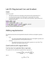
Ôn tập cuối kỳ: Regularized cost and gradient môn Học máy | Trường Đại học Công nghệ, Đại học Quốc gia Hà Nội
70 35